Calculus Connection

Introduction to Trigonometry and Calculus

Trigonometry and calculus are closely connected branches of mathematics. Trigonometry describes angles, triangles, circular motion, and repeating patterns, while calculus investigates how quantities change and how small changes accumulate.

Many physical and mathematical processes involve both ideas.

For example:

• The height of a point on a rotating wheel changes continuously with time.

• The displacement of a vibrating object can be described using sine and cosine functions.

• The slope of a trigonometric graph changes from one point to another.

• The velocity of an oscillating object depends on the rate of change of its position.

• The total energy or displacement associated with a changing quantity can be studied using integration.

Calculus allows us to investigate these situations more precisely.

One of the most important connections is that the derivatives of sine and cosine functions are themselves trigonometric functions.

This remarkable property makes trigonometric functions especially useful in advanced mathematics, physics, and engineering.

What Is Calculus?

Calculus is the branch of mathematics concerned with continuous change and accumulation.

It has two major areas.

Differential Calculus

Differential calculus studies how quickly a quantity changes.

It investigates:

• Slopes of curves.

• Instantaneous rates of change.

• Velocity and acceleration.

• Increasing and decreasing functions.

• Maximum and minimum values.

• Relationships between changing quantities.

Integral Calculus

Integral calculus studies accumulation.

It investigates:

• Areas under curves.

• Total displacement.

• Accumulated quantities.

• Volumes.

• Total change over an interval.

Trigonometric functions are important in both differential and integral calculus because they describe many continuous, repeating processes.

Understanding Limits

A limit describes the value that a function approaches as its input approaches a particular value.

For example, consider:

f(x) = x + 3

As x approaches 2, f(x) approaches 5.

We write:

lim(x → 2) (x + 3) = 5

This means that as x becomes increasingly close to 2, the function values become increasingly close to 5.

Why Limits Matter

Limits form the mathematical foundation of differentiation and integration.

They allow mathematicians to investigate quantities over extremely small intervals.

For example, the slope between two points on a curve can be calculated using:

Average slope = Δy/Δx

As the horizontal separation approaches zero, the average slope may approach a particular value.

That limiting value is the instantaneous slope of the curve.

Limits and Trigonometric Functions

Trigonometric functions are continuous at every point where they are defined.

For example:

lim(x → 0) sin x = 0

lim(x → 0) cos x = 1

These limits follow from the continuity of sine and cosine.

However, some trigonometric limits are more interesting because direct substitution initially produces an undefined expression.

Consider:

lim(x → 0) (sin x)/x

Direct substitution gives:

0/0

This is an indeterminate form, not a numerical answer.

We must investigate how the numerator and denominator behave as x approaches zero.

The Fundamental Trigonometric Limit

One of the most important limits in calculus is:

lim(x → 0) (sin x)/x = 1

This result is valid when x is measured in radians.

Numerical Investigation

Consider the following values:

As x approaches zero from either direction, sin x / x approaches 1.

The expression is undefined at x = 0, but its limit exists.

Why This Limit Is Important

This result is essential for deriving the derivative of the sine function.

It also appears in:

• Wave motion.

• Oscillation models.

• Small-angle approximations.

• Mathematical physics.

• Engineering calculations.

• Advanced trigonometric identities.

Understanding the Limit Geometrically

The fundamental trigonometric limit can be understood using the unit circle.

For small positive angles x, measured in radians, geometric relationships give:

sin x < x < tan x

Dividing by sin x gives:

1 < x/sin x < 1/cos x

Taking reciprocals reverses the inequalities:

cos x < sin x/x < 1

As x approaches zero:

cos x approaches 1.

Therefore, the quantity sin x/x is squeezed between two expressions that both approach 1.

By the Squeeze Theorem:

lim(x → 0) sin x/x = 1

The corresponding result for negative x follows from the symmetry of sine.

This demonstrates how geometry, trigonometry, and limits work together.

Why Radians Are Essential

The fundamental trigonometric limit depends on the unit used to measure angles.

When x is measured in radians:

lim(x → 0) sin x/x = 1

If x represents a numerical angle measured in degrees instead:

lim(x → 0) sin(x°)/x = π/180

This difference has major consequences for calculus.

The familiar derivative formulas for sine and cosine are simplest when angles are measured in radians.

Example

For a very small angle:

sin x ≈ x

provided x is measured in radians.

If:

x = 0.02 radians

then:

sin 0.02 ≈ 0.0199987

This is extremely close to 0.02.

The Small-Angle Approximation

For angles close to zero, measured in radians:

sin x ≈ x

and:

cos x ≈ 1

Another useful approximation is:

tan x ≈ x

These approximations become more accurate as x approaches zero.

Worked Example

Estimate sin 0.03 without a calculator.

Using:

sin x ≈ x

we obtain:

sin 0.03 ≈ 0.03

The actual value is approximately 0.0299955.

The approximation is very accurate.

Applications

Small-angle approximations are useful in:

• Pendulum motion.

• Optics.

• Mechanical vibrations.

• Wave physics.

• Astronomy.

• Engineering design.

Another Important Trigonometric Limit

Consider:

lim(x → 0) (1 − cos x)/x

Direct substitution gives 0/0.

We can simplify using the identity:

1 − cos²x = sin²x

Multiply the numerator and denominator by:

1 + cos x

Then:

(1 − cos x)/x

= (1 − cos²x)/[x(1 + cos x)]

= sin²x/[x(1 + cos x)]

= (sin x/x) × [sin x/(1 + cos x)]

As x approaches zero:

sin x/x → 1

sin x/(1 + cos x) → 0/2

Therefore:

lim(x → 0) (1 − cos x)/x = 0

This result is essential when deriving the derivative of cosine.

Limits Involving Multiples of Angles

The fundamental trigonometric limit can be extended.

For any nonzero constant a:

lim(x → 0) sin(ax)/(ax) = 1

Therefore:

lim(x → 0) sin(ax)/x = a

Worked Example

Evaluate:

lim(x → 0) sin(5x)/x

Rewrite:

sin(5x)/x = 5 × sin(5x)/(5x)

As x approaches zero:

sin(5x)/(5x) → 1

Therefore:

lim(x → 0) sin(5x)/x = 5

Another Example

Evaluate:

lim(x → 0) sin(3x)/sin(7x)

Rewrite:

sin(3x)/sin(7x)

= [sin(3x)/(3x)] × [7x/sin(7x)] × 3/7

Taking the limit:

= 1 × 1 × 3/7

Answer = 3/7

A More Advanced Trigonometric Limit

Consider:

lim(x → 0) (1 − cos x)/x²

Using the identity:

1 − cos x = 2sin²(x/2)

we obtain:

(1 − cos x)/x²

= 2sin²(x/2)/x²

= 1/2 × [sin(x/2)/(x/2)]²

As x approaches zero:

sin(x/2)/(x/2) → 1

Therefore:

lim(x → 0) (1 − cos x)/x² = 1/2

This result is useful in more advanced calculus and mathematical approximations.

From Average Rate of Change to Instantaneous Rate of Change

A rate of change describes how one quantity changes relative to another.

For a function y = f(x), the average rate of change between x = a and x = b is:

Average rate of change = [f(b) − f(a)]/(b − a)

Geometrically, this represents the slope of the straight line connecting two points on the graph.

This line is called a secant line.

Instantaneous Rate of Change

To determine the slope at one particular point, we consider two points that become increasingly close together.

As the separation approaches zero, the secant line approaches a tangent line.

The slope of the tangent line represents the instantaneous rate of change.

This is the central idea of differentiation.

The Derivative

The derivative of a function measures its instantaneous rate of change.

For y = f(x), the derivative is written:

f′(x)

or:

dy/dx

The derivative can be defined using a limit:

f′(x) = lim(h → 0) [f(x + h) − f(x)]/h

This is called the limit definition of the derivative.

The expression:

[f(x + h) − f(x)]/h

represents the average slope over a small interval of width h.

As h approaches zero, the expression approaches the instantaneous slope, provided the limit exists.

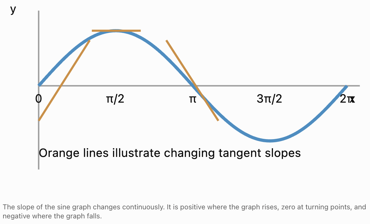
Slopes of Trigonometric Graphs

Consider the sine function:

y = sin x

Its graph repeatedly rises and falls.

At different points, its slope changes.

Important Observations

• Near x = 0, the sine graph is increasing rapidly.

• At x = π/2, the graph reaches a maximum and has zero slope.

• Near x = π, the graph is decreasing rapidly.

• At x = 3π/2, the graph reaches a minimum and has zero slope.

• At x = 2π, the graph is increasing rapidly again.

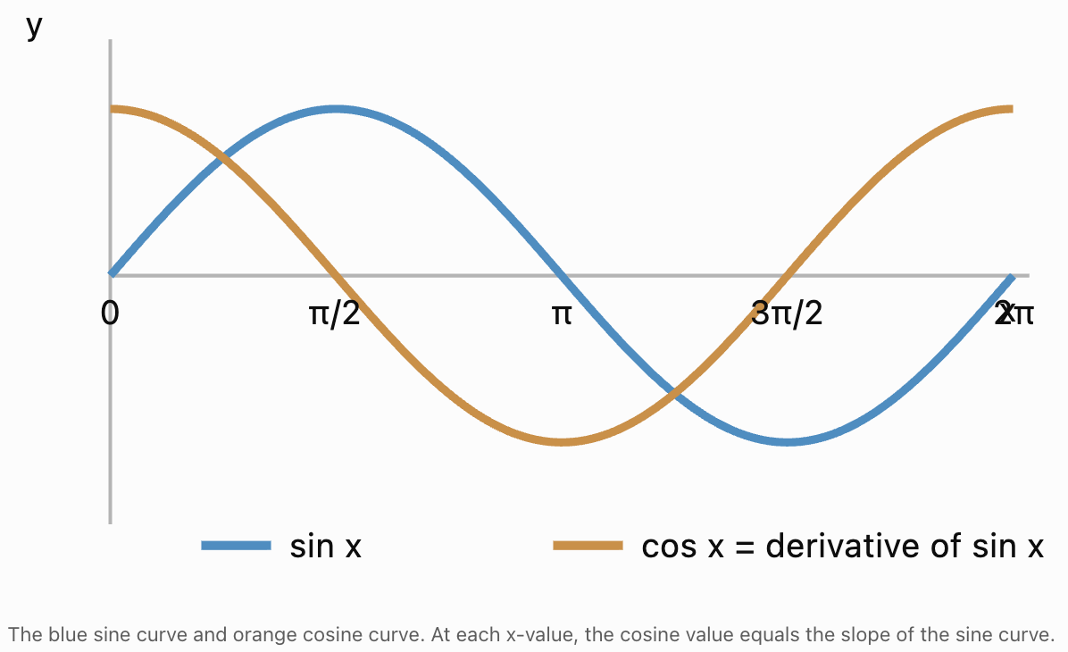
This repeating pattern of slopes can itself be described using a trigonometric function.

Differentiating the Sine Function

One of the fundamental results of calculus is:

d/dx (sin x) = cos x

This means that the instantaneous rate of change of sin x is cos x.

Why Is This True?

Using the definition of the derivative:

f′(x) = lim(h → 0) [sin(x + h) − sin x]/h

Apply the angle addition identity:

sin(x + h) = sin x cos h + cos x sin h

Substituting:

f′(x) = lim(h → 0) [sin x cos h + cos x sin h − sin x]/h

Group the terms:

= lim(h → 0) [sin x(cos h − 1)/h + cos x(sin h/h)]

We know:

lim(h → 0) (cos h − 1)/h = 0

and:

lim(h → 0) sin h/h = 1

Therefore:

f′(x) = sin x × 0 + cos x × 1

f′(x) = cos x

This derivation demonstrates why the fundamental trigonometric limits are so important.

Differentiating the Cosine Function

Another fundamental result is:

d/dx (cos x) = −sin x

This means that the instantaneous rate of change of cosine is negative sine.

Interpreting the Result

Consider:

y = cos x

At x = 0:

cos x is at a maximum.

Its slope is zero.

Since:

−sin 0 = 0

the derivative agrees with the graph.

At x = π/2:

cos x is decreasing most rapidly.

Since:

−sin(π/2) = −1

the slope is −1.

At x = π:

cos x is at a minimum.

Since:

−sin π = 0

the slope is zero again.

The derivative accurately describes the changing slope of the cosine graph.

Comparing Sine, Cosine, and Their Derivatives

Notice that repeated differentiation produces a cycle.

Starting with sin x:

sin x → cos x → −sin x → −cos x → sin x

After four derivatives, the original function returns.

This is a remarkable property of trigonometric functions.

Visualizing the Derivative Relationship

Worked Example: Finding the Slope of a Sine Graph

Consider:

y = sin x

Find the slope at:

x = π/3

Step 1: Differentiate

dy/dx = cos x

Step 2: Substitute

Slope = cos(π/3)

= 1/2

Slope = 0.5

Interpretation

At x = π/3, the sine graph is increasing with an instantaneous slope of 0.5.

Worked Example: Finding the Slope of a Cosine Graph

Consider:

y = cos x

Find the slope at:

x = π/6

Step 1: Differentiate

dy/dx = −sin x

Step 2: Substitute

Slope = −sin(π/6)

= −1/2

Slope = −0.5

Interpretation

At x = π/6, the cosine graph is decreasing with an instantaneous slope of −0.5.

Differentiating Trigonometric Functions with Coefficients

Trigonometric functions often contain constants that change their amplitude or frequency.

Consider:

y = A sin(kx)

Its derivative is:

dy/dx = Ak cos(kx)

Similarly:

y = A cos(kx)

has derivative:

dy/dx = −Ak sin(kx)

These results use the chain rule, an important differentiation technique.

Worked Example

Differentiate:

y = 4 sin(3x)

The amplitude coefficient is 4.

The coefficient inside the sine function is 3.

Therefore:

dy/dx = 4 × 3 cos(3x)

dy/dx = 12 cos(3x)

Another Example

Differentiate:

y = 5 cos(2x)

dy/dx = −5 × 2 sin(2x)

dy/dx = −10 sin(2x)

Understanding the Chain Rule

The chain rule is used to differentiate composite functions.

A composite function contains one function inside another.

For example:

y = sin(3x)

The outer function is sine.

The inner function is 3x.

The chain rule states:

dy/dx = (derivative of outer function) × (derivative of inner function)

For:

y = sin u

where u depends on x:

dy/dx = cos u × du/dx

Example

Differentiate:

y = sin(x²)

Let:

u = x²

Then:

du/dx = 2x

Therefore:

dy/dx = 2x cos(x²)

This illustrates how trigonometric differentiation extends beyond simple functions.

Differentiating Tangent

The tangent function can be written:

tan x = sin x/cos x

Using the quotient rule:

d/dx (tan x) = 1/cos²x

This is often written:

d/dx (tan x) = sec²x

where:

sec x = 1/cos x

The derivative exists wherever cos x is not zero.

Worked Example

Differentiate:

y = 3 tan x

Using the constant multiple rule:

dy/dx = 3 sec²x

This result is useful in advanced calculus, geometry, and engineering.

Rates of Change in Physical Systems

Trigonometric functions often model quantities that vary with time.

For example, the displacement of a vibrating object may be:

x(t) = A sin(ωt)

where:

• x = displacement.

• A = amplitude.

• ω = angular frequency.

• t = time.

The velocity is the derivative of displacement.

v(t) = dx/dt

Therefore:

v(t) = Aω cos(ωt)

Acceleration is the derivative of velocity.

a(t) = dv/dt

Therefore:

a(t) = −Aω² sin(ωt)

Since:

x(t) = A sin(ωt)

we obtain:

a(t) = −ω²x(t)

This relationship is fundamental to simple harmonic motion.

Worked Example: Displacement, Velocity, and Acceleration

A vibrating object moves according to:

x(t) = 0.05 sin(4πt)

where displacement is measured in metres and time in seconds.

Find expressions for velocity and acceleration.

Step 1: Identify the Constants

A = 0.05 m

ω = 4π rad/s

Step 2: Differentiate to Find Velocity

v(t) = 0.05 × 4π cos(4πt)

v(t) = 0.20π cos(4πt)

Step 3: Differentiate to Find Acceleration

a(t) = −0.20π × 4π sin(4πt)

a(t) = −0.80π² sin(4πt)

Step 4: Calculate Maximum Values

Maximum speed:

v_max = Aω

= 0.05 × 4π

v_max ≈ 0.628 m/s

Maximum acceleration magnitude:

a_max = Aω²

= 0.05 × (4π)²

a_max ≈ 7.90 m/s²

Interpretation

The object moves periodically, but its velocity and acceleration change continuously.

Calculus allows these quantities to be determined directly from the displacement function.

Circular Motion and Calculus

Consider a point moving around a circle of radius r at constant angular velocity ω.

Its coordinates are:

x(t) = r cos(ωt)

y(t) = r sin(ωt)

Differentiate to find the velocity components:

vₓ(t) = −rω sin(ωt)

vᵧ(t) = rω cos(ωt)

Differentiate again to find acceleration:

aₓ(t) = −rω² cos(ωt)

aᵧ(t) = −rω² sin(ωt)

The acceleration vector points toward the centre of the circle.

Its magnitude is:

a = rω²

This is the familiar centripetal acceleration formula.

Why This Matters

Trigonometry describes the position of a rotating object.

Calculus describes its velocity and acceleration.

Together, they provide a complete mathematical model of uniform circular motion.

Tangent Lines and Trigonometric Functions

A tangent line touches a smooth curve at a particular point and has the same instantaneous slope as the curve there.

For a function:

y = f(x)

the tangent line at x = a has slope:

m = f′(a)

The equation of the tangent line is:

y − f(a) = m(x − a)

Worked Example

Find the tangent line to:

y = sin x

at:

x = 0

Step 1: Find the Point

sin 0 = 0

The point is:

(0, 0)

Step 2: Find the Derivative

f′(x) = cos x

At x = 0:

m = cos 0

m = 1

Step 3: Write the Tangent Equation

y − 0 = 1(x − 0)

y = x

Interpretation

Near the origin, the sine curve is closely approximated by the straight line y = x.

This explains the small-angle approximation:

sin x ≈ x

for small angles in radians.

Increasing and Decreasing Trigonometric Functions

The derivative indicates whether a function is increasing or decreasing.

If:

f′(x) > 0

the function is increasing.

If:

f′(x) < 0

the function is decreasing.

If:

f′(x) = 0

the function has a stationary point, which may be a maximum, minimum, or another type of stationary point.

Example: Sine Function

For:

f(x) = sin x

the derivative is:

f′(x) = cos x

Between 0 and π/2:

cos x is positive.

Therefore, sin x is increasing.

Between π/2 and 3π/2:

cos x is negative.

Therefore, sin x is decreasing.

Between 3π/2 and 2π:

cos x is positive.

Therefore, sin x is increasing again.

This demonstrates how differentiation can be used to analyse trigonometric graphs.

Maximum and Minimum Values

Differentiation can help locate maximum and minimum values.

For a differentiable function, an interior local maximum or minimum must occur where the derivative is zero.

Consider:

f(x) = 3 sin x + 2

Differentiate:

f′(x) = 3 cos x

Set the derivative equal to zero:

3 cos x = 0

cos x = 0

Within the interval 0 ≤ x ≤ 2π:

x = π/2 or 3π/2

Evaluate the function.

At x = π/2:

f(π/2) = 3(1) + 2

f = 5

At x = 3π/2:

f(3π/2) = 3(−1) + 2

f = −1

Therefore:

Maximum value = 5

Minimum value = −1

These results also agree with the amplitude and vertical shift of the original function.

The Second Derivative

The second derivative describes the rate of change of the first derivative.

It is written:

f″(x)

For a position function, the first derivative gives velocity and the second derivative gives acceleration.

Example

Consider:

f(x) = sin x

First derivative:

f′(x) = cos x

Second derivative:

f″(x) = −sin x

Therefore:

f″(x) = −f(x)

This relationship is particularly important in wave motion and oscillations.

Physical Connection

Many oscillating systems satisfy equations of the form:

d²x/dt² = −ω²x

This means acceleration is proportional to displacement but acts in the opposite direction.

Sine and cosine functions naturally satisfy this relationship.

Introduction to Integration

Differentiation investigates rates of change.

Integration investigates accumulation.

An indefinite integral finds a family of functions whose derivative equals a given function.

For example:

Since:

d/dx (sin x) = cos x

we know:

∫ cos x dx = sin x + C

Similarly:

Since:

d/dx (cos x) = −sin x

we obtain:

∫ sin x dx = −cos x + C

Here, C is the constant of integration.

Why Is C Needed?

The derivative of a constant is zero.

Therefore, functions that differ only by a constant have the same derivative.

For example:

sin x

sin x + 3

sin x − 7

all have derivative cos x.

Definite Integrals and Area

A definite integral calculates signed accumulation over an interval.

It can represent the signed area between a graph and the x-axis.

Consider:

∫₀^π sin x dx

Using:

∫ sin x dx = −cos x + C

we evaluate:

[−cos x] from 0 to π

= −cos π − (−cos 0)

= 1 + 1

= 2

Therefore:

∫₀^π sin x dx = 2

Since sin x is nonnegative over this interval, the signed area is also the ordinary area between the curve and the x-axis.

Integration in Physics

Integration can be used to calculate displacement from velocity.

Suppose:

v(t) = 3 cos(2t)

Velocity is the derivative of displacement.

Therefore:

x(t) = ∫3 cos(2t) dt

Using the reverse chain rule:

x(t) = 1.5 sin(2t) + C

If the initial position is zero:

x(0) = 0

Then:

C = 0

Therefore:

x(t) = 1.5 sin(2t)

This illustrates how calculus can move between displacement and velocity models.

Trigonometric Functions in Advanced Mathematics

Trigonometric functions appear in many advanced mathematical topics.

Differential Equations

Differential equations describe relationships between functions and their derivatives.

They are used to model:

• Oscillations.

• Waves.

• Electrical circuits.

• Mechanical vibrations.

• Population changes.

• Dynamic systems.

Sine and cosine functions frequently appear as solutions to differential equations involving oscillation.

Fourier Analysis

Fourier analysis studies how complicated signals can be represented using combinations of sine and cosine functions.

It is used in:

• Sound processing.

• Image compression.

• Medical imaging.

• Communications.

• Vibration analysis.

Complex Numbers

Euler's formula connects trigonometry with complex numbers:

e^(ix) = cos x + i sin x

where i² = −1.

This relationship is fundamental in advanced mathematics, electrical engineering, and signal processing.

Taylor Series

Taylor series allow functions to be approximated using polynomials.

For angles measured in radians:

sin x = x − x³/3! + x⁵/5! − ...

cos x = 1 − x²/2! + x⁴/4! − ...

These series explain why:

sin x ≈ x

and:

cos x ≈ 1 − x²/2

for small x.

Mathematical Modelling

Trigonometric calculus is used to model periodic phenomena in:

• Physics.

• Engineering.

• Astronomy.

• Economics.

• Biology.

• Computer science.

Choosing the Correct Calculus Method

Common Mistakes

Using degrees instead of radians

Standard trigonometric derivative and limit formulas assume angles are measured in radians.

Assuming 0/0 is equal to zero

The expression 0/0 is indeterminate and requires further analysis.

Confusing a limit with direct substitution

A function may be undefined at a point even when its limit exists there.

Confusing average and instantaneous rates of change

Average rates use an interval, while instantaneous rates describe change at a particular point.

Forgetting the negative sign when differentiating cosine

The derivative of cos x is −sin x, not sin x.

Forgetting the chain rule

The derivative of sin(3x) is 3 cos(3x), not simply cos(3x).

Confusing a function with its derivative

The derivative describes the slope of the original function, not its height.

Assuming every stationary point is a maximum

A stationary point may be a maximum, minimum, or neither.

Ignoring the constant of integration

Indefinite integrals require a constant because many functions share the same derivative.

Confusing signed area with total geometric area

A definite integral can be negative when the graph lies below the x-axis.

Applying small-angle approximations to large angles

The approximations sin x ≈ x and tan x ≈ x are only accurate when x is sufficiently close to zero in radians.

Key Terms

• Calculus: The branch of mathematics concerned with rates of change and accumulation.

• Differential Calculus: The study of derivatives and instantaneous rates of change.

• Integral Calculus: The study of accumulation and integration.

• Limit: The value approached by a function as its input approaches a specified value.

• Continuity: A property describing functions without a break at a particular point.

• Indeterminate Form: An expression such as 0/0 that does not directly determine a limit.

• Fundamental Trigonometric Limit: The result that sin x/x approaches 1 as x approaches zero in radians.

• Squeeze Theorem: A method for determining a limit by bounding a function between two functions with the same limit.

• Radian: An angular unit defined using arc length and radius.

• Small-Angle Approximation: An approximation that simplifies trigonometric functions for angles near zero.

• Average Rate of Change: The change in output divided by the change in input over an interval.

• Instantaneous Rate of Change: The rate at which a function changes at a particular point.

• Derivative: A function that describes instantaneous rates of change.

• Differentiation: The process of finding a derivative.

• Secant Line: A line passing through two points on a curve.

• Tangent Line: A line whose slope matches the instantaneous slope of a curve at a point.

• Chain Rule: A differentiation rule for composite functions.

• Composite Function: A function formed by applying one function to the output of another.

• First Derivative: The instantaneous rate of change of a function.

• Second Derivative: The rate of change of the first derivative.

• Stationary Point: A point where the derivative is zero.

• Critical Point: A point where the derivative is zero or does not exist, provided the point is in the function's domain.

• Local Maximum: A function value greater than or equal to nearby values.

• Local Minimum: A function value less than or equal to nearby values.

• Integration: The mathematical process of finding antiderivatives or accumulated quantities.

• Indefinite Integral: A family of antiderivatives.

• Definite Integral: A quantity representing signed accumulation over an interval.

• Constant of Integration: An arbitrary constant added to an indefinite integral.

• Differential Equation: An equation involving a function and one or more of its derivatives.

• Fourier Analysis: The study of representing signals using combinations of sinusoidal functions.

• Taylor Series: A polynomial series used to represent or approximate a function.

• Euler's Formula: A relationship connecting exponential functions, complex numbers, and trigonometric functions.

• Simple Harmonic Motion: Oscillation in which acceleration is proportional to displacement and directed toward equilibrium.

Key Takeaways

• Trigonometry and calculus are closely connected because trigonometric functions describe continuously changing, periodic quantities.

• Calculus investigates instantaneous rates of change and accumulation.

• Limits provide the mathematical foundation for derivatives and integrals.

• The fundamental trigonometric limit is lim(x → 0) sin x/x = 1 when x is measured in radians.

• Another important limit is lim(x → 0) (1 − cos x)/x = 0.

• The small-angle approximation sin x ≈ x is useful when x is close to zero in radians.

• Average rate of change is calculated over an interval.

• Instantaneous rate of change is represented by the derivative.

• The derivative describes the slope of a curve at a particular point.

• The derivative of sin x is cos x.

• The derivative of cos x is −sin x.

• Repeated differentiation of sine and cosine produces a repeating cycle.

• The chain rule allows composite trigonometric functions to be differentiated.

• Derivatives can identify where functions are increasing or decreasing.

• Stationary points can be investigated to find maximum and minimum values.

• The first derivative of displacement gives velocity.

• The second derivative of displacement gives acceleration.

• Circular motion can be analysed using trigonometric position functions and their derivatives.

• Simple harmonic motion is closely connected to second-order differential equations.

• Integration reverses differentiation and can calculate accumulated quantities.

• Fourier analysis uses sine and cosine functions to represent complex signals.

• Euler's formula connects trigonometric functions with complex numbers and exponential functions.

• Taylor series provide polynomial approximations for trigonometric functions.

• Trigonometric calculus is widely used in physics, engineering, signal processing, and advanced mathematics.

Check Your Understanding

Recall and Understanding

1. Explain the difference between differential calculus and integral calculus.

2. Define a limit and explain why limits are important in calculus.

3. State the fundamental trigonometric limit involving sin x/x.

4. Explain why radians are important when differentiating trigonometric functions.

5. Describe the relationship between a function's graph and its derivative.

Application

6. Evaluate lim(x → 0) sin(4x)/x.

7. Evaluate lim(x → 0) sin(2x)/sin(5x).

8. Differentiate y = 6 sin x.

9. Differentiate y = 4 cos(3x).

10. Find the slope of y = sin x at x = π/4.

Analysis and Challenge

11. Use the fundamental trigonometric limit to evaluate lim(x → 0) (1 − cos x)/x².

12. A vibrating object has displacement x(t) = 0.08 sin(5t). Find expressions for its velocity and acceleration, then calculate its maximum speed and acceleration magnitude.

13. A point moves around a circle according to x(t) = 3 cos(2t) and y(t) = 3 sin(2t). Find its velocity components and calculate its constant speed.

14. Find the stationary points of f(x) = 2 sin x + 1 over the interval 0 ≤ x ≤ 2π, and classify them as maxima or minima.

15. Explain how trigonometric functions, differentiation, integration, and differential equations work together to describe oscillating physical systems.

Final Summary

Trigonometry provides mathematical models for angles, circular motion, and periodic behaviour, while calculus explains how these quantities change and accumulate.

Limits establish the foundations of differentiation, including the important relationship that sin x/x approaches 1 as x approaches zero in radians.

Differentiation reveals that the rate of change of sine is cosine, while the rate of change of cosine is negative sine.

These relationships make trigonometric functions particularly useful for describing velocity, acceleration, circular motion, and oscillations.

Integration allows accumulated quantities to be calculated and provides a way to recover displacement from velocity.

More advanced topics, including differential equations, Fourier analysis, Taylor series, and complex numbers, build on these connections.

The central principle is that trigonometric functions describe repeating patterns, while calculus provides the tools needed to understand how those patterns change, how quickly they change, and how their effects accumulate over time.