Applications of Advanced Trigonometry
| Site: | Young Education |
| Cours: | Advanced Trigonomitry |
| Livre: | Applications of Advanced Trigonometry |
| Imprimé par: | Guest user |
| Date: | lundi 9 novembre 2026, 16:37 |
1. Wave Motion
Learning outcomes
- I can model wave behaviour using trigonometric functions.
- I can interpret phase relationships.
- I can analyse interference patterns.
- I can solve problems involving oscillations.
- I can connect mathematical models to physical systems.
Wave Motion
Introduction to Wave Motion
Waves are disturbances that transfer energy from one location to another. They occur throughout nature and technology, including sound, light, water waves, earthquakes, radio signals, and vibrations in mechanical systems.
Many waves exhibit repeating patterns that can be described mathematically using sine and cosine functions.
Trigonometric models allow us to calculate wave displacement, amplitude, frequency, wavelength, phase, and interference.
For example, mathematics can help us determine:
-
How far a vibrating object moves from its equilibrium position.
-
How frequently a wave oscillates.
-
Whether two waves reinforce or cancel each other.
-
How the position of a wave changes with time.
-
How wave speed depends on frequency and wavelength.
-
How mathematical wave models relate to real physical systems.
Wave motion provides one of the most important applications of trigonometry in physics and engineering.


Understanding Wave Motion
A wave is a disturbance that travels through a medium or through space, transferring energy.
Two major types of waves are transverse and longitudinal waves.
Transverse Waves
In a transverse wave, the oscillations are perpendicular to the direction of wave propagation.
Examples include:
-
Waves on a stretched string.
-
Electromagnetic waves.
-
Certain seismic waves.
Longitudinal Waves
In a longitudinal wave, the oscillations are parallel to the direction of propagation.
Examples include:
-
Sound waves in air.
-
Compression waves in springs.
-
Certain seismic waves.
Both types of waves can exhibit sinusoidal behaviour, although the physical meaning of displacement differs.


Describing Waves Using Trigonometric Functions
A sinusoidal oscillation can be modelled using:
y = A sin(ωt + φ)
or:
y = A cos(ωt + φ)
where:
-
y = displacement from equilibrium.
-
A = amplitude.
-
ω = angular frequency.
-
t = time.
-
φ = initial phase angle.
The sine and cosine functions are useful because they repeat regularly and smoothly.
Example
Consider:
y = 4 sin(2πt)
This describes an oscillation with:
-
Amplitude = 4 units.
-
Angular frequency = 2π rad/s.
-
Frequency = 1 Hz.
-
Period = 1 s.
-
Initial phase = 0 radians.
The displacement changes continuously between −4 and +4.
Visualizing a Sinusoidal Wave
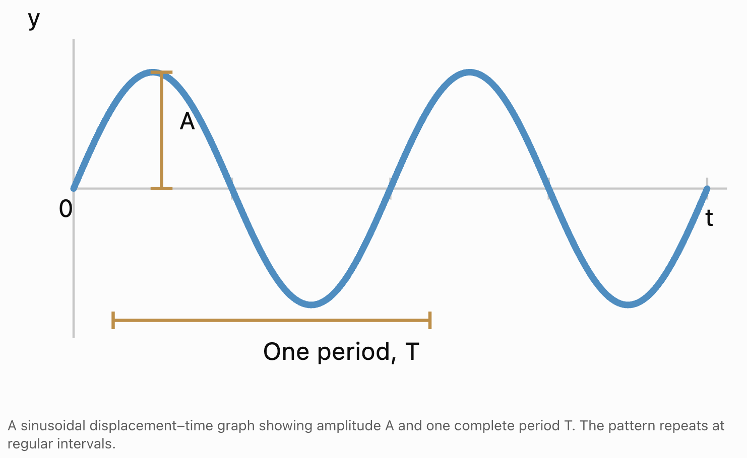
Important Features
Equilibrium position: The central position about which the oscillation occurs.
Amplitude: The maximum displacement from equilibrium.
Crest: The highest point of a transverse wave.
Trough: The lowest point of a transverse wave.
Period: The time required for one complete oscillation.
Frequency: The number of complete oscillations per second.
Amplitude
The amplitude of a wave is its maximum displacement from equilibrium.
For:
y = A sin(ωt + φ)
the amplitude is:
|A|
Example
Consider:
y = 7 sin(3t)
The amplitude is:
7 units
The displacement varies between:
−7 and +7
Negative Coefficients
For:
y = −5 cos(2t)
the amplitude is still:
5 units
The negative sign reflects the graph vertically; it does not produce a negative amplitude.
Physical Meaning
Amplitude may represent:
-
Displacement of a vibrating string.
-
Pressure variation in a sound wave.
-
Electric-field strength in an electromagnetic wave.
-
Height variation of a water surface.
The precise physical meaning depends on the system being modelled.
Period and Frequency
The period, T, is the time required for one complete oscillation.
The frequency, f, is the number of oscillations per second.
Their relationship is:
f = 1/T
and:
T = 1/f
Frequency is measured in hertz (Hz).
One hertz means one complete oscillation per second.
Worked Example
A wave completes 25 oscillations in five seconds.
Frequency:
f = 25/5
f = 5 Hz
Period:
T = 1/5
T = 0.2 s
The wave completes five oscillations each second.
Angular Frequency
Angular frequency describes how quickly the phase of an oscillation changes.
It is represented by ω.
ω = 2πf
Since f = 1/T:
ω = 2π/T
Angular frequency is measured in radians per second.
Worked Example
A vibrating object has a frequency of 8 Hz.
Calculate its angular frequency.
ω = 2π × 8
ω = 16π rad/s
Approximately:
ω ≈ 50.27 rad/s
Relationship to the Graph
For:
y = A sin(ωt)
the period is:
T = 2π/|ω|
A larger angular frequency produces more oscillations in the same time interval.
Worked Example: Analysing a Trigonometric Model
Consider:
y = 6 sin(4πt)
where y is measured in centimetres and t in seconds.
Find the amplitude, period, frequency, and angular frequency.
Amplitude
A = 6 cm
Angular Frequency
ω = 4π rad/s
Period
T = 2π/(4π)
T = 0.5 s
Frequency
f = 1/0.5
f = 2 Hz
Interpretation
The object moves between −6 cm and +6 cm and completes two oscillations every second.
Phase and Phase Angle
The phase of an oscillation describes its position within the repeating cycle.
For:
y = A sin(ωt + φ)
the quantity:
ωt + φ
is the instantaneous phase.
The constant φ is the initial phase angle.
Phase is measured in radians or degrees.
Common Phase Angles
|
Phase angle |
Radians |
Fraction of cycle |
|---|---|---|
|
0° |
0 |
0 |
|
90° |
π/2 |
1/4 |
|
180° |
π |
1/2 |
|
270° |
3π/2 |
3/4 |
|
360° |
2π |
1 |
A phase change of 2π radians represents one complete cycle.
Phase Shifts
Consider:
y₁ = sin(ωt)
and:
y₂ = sin(ωt + π/2)
The second oscillation has a phase lead of π/2 radians.
This corresponds to one-quarter of a cycle.
For a positive angular frequency, the graph of y₂ is shifted to the left by:
Δt = (π/2)/ω
General Formula
For two oscillations of the same angular frequency:
Phase difference = Δφ
The corresponding time difference is:
Δt = |Δφ|/ω
This uses a chosen phase difference, typically reduced to the interval from 0 to π when comparing the smallest separation between corresponding features.
Example
Two oscillations have frequency 10 Hz and a phase difference of π/2 radians.
Angular frequency:
ω = 2π × 10 = 20π rad/s
Time difference:
Δt = (π/2)/(20π)
Δt = 0.025 s
The oscillations differ by 0.025 seconds, or one-quarter of their 0.1-second period.
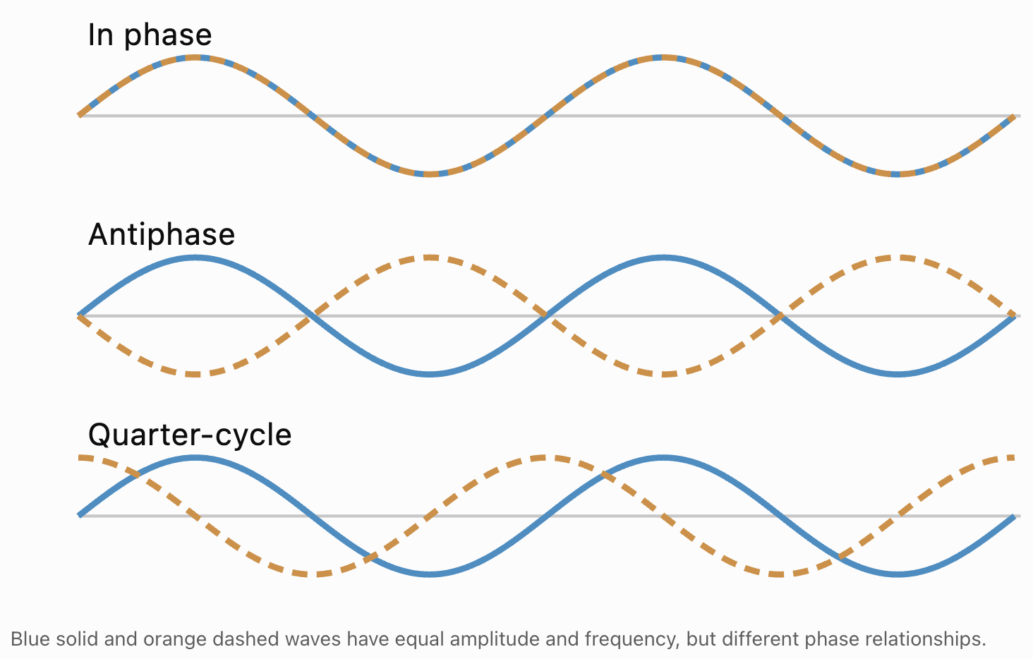
Comparing Phase Relationships
Two waves may be in phase, out of phase, or have an intermediate phase difference.
In Phase
Two waves are in phase when corresponding crests, troughs, and zero crossings occur together.
Their phase difference is:
Δφ = 0, or any whole multiple of 2π
In Antiphase
Two waves are in antiphase when one wave reaches a crest as the other reaches a trough.
Their phase difference is:
Δφ = π, or an odd multiple of π
Intermediate Phase Differences
A phase difference of π/2 corresponds to a quarter-cycle separation.
Wavelength and Wave Speed
The wavelength, λ, is the distance between two consecutive points in the same phase, such as two neighbouring crests.
The wave speed, v, is the speed at which the wave pattern propagates.
The relationship is:
v = fλ
where:
-
v = wave speed in m/s.
-
f = frequency in Hz.
-
λ = wavelength in metres.
Rearranging
f = v/λ
λ = v/f
Worked Example
A wave travels at 24 m/s and has a frequency of 6 Hz.
Find its wavelength.
λ = v/f
= 24/6
λ = 4 m
The distance between consecutive crests is four metres.
The Travelling Wave Equation
A wave travelling through space can be represented using both position and time.
For a sinusoidal wave travelling in the positive x-direction:
y(x,t) = A sin(kx − ωt + φ)
where:
-
A = amplitude.
-
k = wave number.
-
x = position.
-
ω = angular frequency.
-
t = time.
-
φ = phase constant.
The wave number is:
k = 2π/λ
Wave Speed
The speed of the wave is:
v = ω/k
Since:
ω = 2πf
and:
k = 2π/λ
then:
v = (2πf)/(2π/λ)
Therefore:
v = fλ
Direction of Propagation
For positive k and ω:
kx − ωt describes motion in the positive x-direction.
kx + ωt describes motion in the negative x-direction.
This distinction is important when interpreting travelling-wave equations.
Worked Example: Analysing a Travelling Wave
Consider the wave equation:
y(x,t) = 0.04 sin(2πx − 8πt)
where x and y are measured in metres and t in seconds.
Determine the amplitude, wavelength, frequency, period, and wave speed.
Step 1: Identify the Amplitude
A = 0.04 m
Amplitude = 4 cm
Step 2: Identify the Wave Number
k = 2π rad/m
Since:
k = 2π/λ
λ = 2π/(2π)
λ = 1 m
Step 3: Identify the Angular Frequency
ω = 8π rad/s
Since:
ω = 2πf
f = 8π/(2π)
f = 4 Hz
Step 4: Calculate the Period
T = 1/f
T = 0.25 s
Step 5: Calculate the Wave Speed
v = fλ
= 4 × 1
v = 4 m/s
Interpretation
The wave has an amplitude of 4 cm, completes four oscillations each second, and travels in the positive x-direction at 4 m/s.
The Principle of Superposition
When two or more waves overlap, their individual displacements add together.
This is called the principle of superposition.
For two waves:
y_resultant = y₁ + y₂
The waves may reinforce each other or partially or completely cancel.
Superposition applies to linear wave systems, where the disturbances do not permanently alter each other's propagation.
Constructive Interference
Constructive interference occurs when overlapping waves reinforce each other.
For two identical sinusoidal waves that are in phase:
y₁ = A sin(ωt)
y₂ = A sin(ωt)
Their resultant displacement is:
y_resultant = 2A sin(ωt)
The resultant amplitude is:
A_resultant = 2A
Example
Two waves each have an amplitude of 3 cm and are perfectly in phase.
Resultant amplitude:
3 + 3
= 6 cm
The maximum displacement is doubled.

Destructive Interference
Destructive interference occurs when overlapping waves oppose each other.
For two identical sinusoidal waves in antiphase:
y₁ = A sin(ωt)
y₂ = A sin(ωt + π)
Since:
sin(θ + π) = −sin(θ)
then:
y₂ = −A sin(ωt)
Therefore:
y_resultant = 0
The two waves cancel completely.
Important Condition
Complete cancellation requires waves with equal amplitudes and a phase difference of an odd multiple of π.
If the amplitudes differ, the waves may only partially cancel.
For example, two waves with amplitudes of 5 cm and 3 cm in antiphase produce a resultant amplitude of:
|5 − 3| = 2 cm
Interference and Phase Difference
When two waves have the same frequency and equal amplitude A, but a phase difference Δφ, their resultant amplitude is:
A_resultant = 2A|cos(Δφ/2)|
This follows from the trigonometric identity:
sin α + sin β = 2 sin[(α + β)/2] cos[(α − β)/2]
Worked Example
Two waves each have an amplitude of 4 cm and a phase difference of 120°.
Calculate the resultant amplitude.
A_resultant = 2 × 4 × |cos(120°/2)|
= 8 × |cos 60°|
= 8 × 0.5
A_resultant = 4 cm
Interpretation
The resultant amplitude is smaller than the maximum possible amplitude of 8 cm because the waves are not in phase.
Comparing Phase Differences
|
Phase difference |
Resultant amplitude for equal waves |
|---|---|
|
0° |
2A |
|
60° |
√3 A |
|
90° |
√2 A |
|
120° |
A |
|
180° |
0 |
This relationship is useful when analysing interference patterns.
Path Difference and Interference
When waves travel different distances before meeting, they may arrive with different phases.
The path difference, Δd, is the difference between the distances travelled.
For coherent waves with the same wavelength:
Δφ = 2πΔd/λ
This assumes the sources begin in phase. Otherwise, the initial phase difference must also be included.
Constructive Interference
For in-phase sources, constructive interference occurs when:
Δd = mλ
where m is an integer.
Examples include:
0, λ, 2λ, 3λ ...
Destructive Interference
For in-phase sources, destructive interference occurs when:
Δd = (m + 1/2)λ
Examples include:
λ/2, 3λ/2, 5λ/2 ...
Worked Example
Two coherent water waves have a wavelength of 0.8 m.
At a particular point, the path difference is 1.2 m.
Calculate:
Δd/λ = 1.2/0.8
= 1.5
The path difference is 1.5 wavelengths.
Therefore, the waves arrive in antiphase and produce destructive interference if their amplitudes are equal.

Standing Waves
A standing wave is formed when two waves of equal frequency and amplitude travel in opposite directions and interfere.
For example:
y₁ = A sin(kx − ωt)
y₂ = A sin(kx + ωt)
Adding the waves gives:
y = 2A sin(kx) cos(ωt)
This describes a standing wave.
Unlike a travelling wave, the pattern does not move along the medium.
Instead, different positions oscillate with different amplitudes.
Nodes
A node is a point where the displacement is always zero.
For the standing-wave equation:
sin(kx) = 0
Therefore:
kx = nπ
Since k = 2π/λ:
x = nλ/2
Adjacent nodes are separated by:
λ/2
Antinodes
An antinode is a point where the oscillation amplitude is greatest.
Antinodes occur halfway between adjacent nodes.
Examples of Standing Waves
-
Vibrating guitar strings.
-
Organ pipes.
-
Resonating air columns.
-
Certain microwave cavities.
-
Vibrations in mechanical structures.

Standing Waves on a String
Consider a string fixed at both ends.
Both ends must be nodes.
For a string of length L, the allowed wavelengths are:
λₙ = 2L/n
where:
n = 1, 2, 3, ...
The corresponding frequencies are:
fₙ = nv/(2L)
where v is the wave speed.
Fundamental Frequency
For n = 1:
f₁ = v/(2L)
This is the lowest resonant frequency.
Harmonics
Higher frequencies are integer multiples of the fundamental frequency:
f₂ = 2f₁
f₃ = 3f₁
f₄ = 4f₁
Worked Example
A guitar string has a length of 0.75 m.
The wave speed along the string is 120 m/s.
Calculate the fundamental frequency.
f₁ = v/(2L)
= 120/(2 × 0.75)
= 120/1.5
f₁ = 80 Hz
The second harmonic is:
f₂ = 160 Hz
The third harmonic is:
f₃ = 240 Hz
These frequencies help determine the sound produced by the vibrating string.
Simple Harmonic Motion
Simple harmonic motion (SHM) is a type of oscillation in which acceleration is proportional to displacement and directed toward equilibrium.
Mathematically:
a = −ω²x
The negative sign indicates that acceleration acts toward the equilibrium position.
SHM can be represented using:
x(t) = A cos(ωt + φ)
Examples include:
-
An ideal mass–spring system.
-
A simple pendulum at small angles.
-
Certain vibrating mechanical components.
-
Oscillating electrical systems.
Displacement, Velocity, and Acceleration in SHM
For an object undergoing simple harmonic motion:
x(t) = A cos(ωt + φ)
Velocity is the rate of change of displacement:
v(t) = −Aω sin(ωt + φ)
Acceleration is the rate of change of velocity:
a(t) = −Aω² cos(ωt + φ)
Therefore:
a(t) = −ω²x(t)
Maximum Values
Maximum displacement:
x_max = A
Maximum speed:
v_max = Aω
Maximum acceleration magnitude:
a_max = Aω²
Phase Relationships
-
Velocity differs in phase from displacement by one-quarter of a cycle.
-
Acceleration is in antiphase with displacement.
-
Speed is greatest at equilibrium.
-
Acceleration magnitude is greatest at maximum displacement.
Worked Example: Oscillating Mass
A mass moves according to:
x(t) = 0.08 cos(5t)
where displacement is measured in metres and time in seconds.
Amplitude
A = 0.08 m
= 8 cm
Angular Frequency
ω = 5 rad/s
Period
T = 2π/5
T ≈ 1.26 s
Maximum Speed
v_max = Aω
= 0.08 × 5
v_max = 0.40 m/s
Maximum Acceleration
a_max = Aω²
= 0.08 × 25
a_max = 2.0 m/s²
Interpretation
The mass oscillates 8 cm on either side of equilibrium, reaches a maximum speed of 0.40 m/s, and experiences a maximum acceleration magnitude of 2.0 m/s².
Mass–Spring Systems
An ideal mass attached to a spring can undergo simple harmonic motion.
Hooke's Law states:
F = −kx
where:
-
F = restoring force.
-
k = spring constant.
-
x = displacement from equilibrium.
Using Newton's Second Law:
ma = −kx
Therefore:
a = −(k/m)x
Comparing this with:
a = −ω²x
gives:
ω = √(k/m)
The period is:
T = 2π√(m/k)
Worked Example
A mass of 0.50 kg is attached to a spring with spring constant 200 N/m.
Calculate the period.
T = 2π√(0.50/200)
= 2π√0.0025
= 2π × 0.05
T ≈ 0.314 s
Interpretation
Increasing the mass increases the period.
Increasing the spring constant decreases the period.

Pendulum Motion
A simple pendulum consists of a mass suspended from a fixed point by a string or rod.
For small angular displacements, the pendulum approximately undergoes simple harmonic motion.
Its period is:
T = 2π√(L/g)
where:
-
L = pendulum length.
-
g = gravitational field strength.
Worked Example
A pendulum has a length of 1.0 m.
Take:
g = 9.81 m/s²
Calculate its period.
T = 2π√(1.0/9.81)
T ≈ 2.01 s
Interpretation
A longer pendulum has a longer period.
For small oscillations, the period is approximately independent of the mass of the pendulum bob.
The small-angle assumption becomes less accurate for large oscillations.

Energy in Oscillatory Systems
In an ideal undamped mass–spring system, mechanical energy is conserved.
Energy continuously transfers between:
-
Elastic potential energy.
-
Kinetic energy.
Elastic Potential Energy
Eₚ = 1/2 kx²
Kinetic Energy
Eₖ = 1/2 mv²
Total Mechanical Energy
E_total = 1/2 kA²
where A is the amplitude.
At Maximum Displacement
-
Speed is zero.
-
Kinetic energy is zero.
-
Elastic potential energy is maximum.
At Equilibrium
-
Speed is maximum.
-
Kinetic energy is maximum.
-
Elastic potential energy is minimum.
Real Systems
Real oscillations lose energy through friction, air resistance, and other dissipative processes.
As a result, their amplitudes may decrease over time.
Damped Oscillations
A damped oscillation gradually decreases in amplitude because energy is transferred away from the oscillating system.
A common model for underdamped motion is:
x(t) = A₀e^(−bt) cos(ω_dt + φ)
where:
-
A₀ = initial amplitude.
-
b = positive decay constant.
-
ω_d = damped angular frequency.
-
φ = phase constant.
The exponential factor:
e^(−bt)
causes the amplitude to decrease over time.
Applications
Damping is important in:
-
Vehicle suspension systems.
-
Building vibration control.
-
Mechanical shock absorbers.
-
Seismic protection.
-
Precision instruments.

Resonance
Resonance occurs when a system responds strongly to a periodic driving force whose frequency is near the system's natural frequency.
Examples include:
-
Musical instruments.
-
Mechanical structures.
-
Electrical circuits.
-
Acoustic systems.
Natural Frequency
The natural frequency is the frequency at which a system tends to oscillate when disturbed.
For an ideal mass–spring system:
f₀ = (1/2π)√(k/m)
Resonance and Amplitude
When a driving frequency approaches the resonant frequency, the oscillation amplitude may increase substantially.
Damping limits the maximum response.
Engineering Importance
Engineers must consider resonance when designing:
-
Bridges.
-
Buildings.
-
Rotating machinery.
-
Aircraft components.
-
Vehicle suspension systems.
Excessive resonance can produce damaging vibrations.
Beats and Interference Between Different Frequencies
When two waves have slightly different frequencies, their superposition can produce beats.
Beats are periodic changes in the amplitude of the combined wave.
For two frequencies f₁ and f₂:
f_beat = |f₁ − f₂|
Worked Example
Two tuning forks produce frequencies of:
440 Hz and 444 Hz.
Calculate the beat frequency.
f_beat = |444 − 440|
f_beat = 4 Hz
The combined sound becomes louder and softer four times per second.
Applications
Beat frequencies are used in:
-
Tuning musical instruments.
-
Acoustic measurements.
-
Signal processing.
-
Frequency comparison.

Connecting Wave Models to Physical Systems
Trigonometric wave models appear throughout science and engineering.
|
Physical system |
Mathematical application |
|---|---|
|
Sound waves |
Frequency, amplitude, interference, beats |
|
Water waves |
Wavelength, speed, phase, superposition |
|
Light waves |
Interference, diffraction, phase difference |
|
Guitar strings |
Standing waves and harmonics |
|
Pendulums |
Periodic motion and small-angle SHM |
|
Springs |
Displacement, velocity, acceleration |
|
Electrical circuits |
Alternating voltage and current |
|
Buildings |
Resonance and damping |
|
Communication systems |
Signal phase, frequency, modulation |
Alternating Current
An alternating voltage can be modelled as:
V(t) = V₀ sin(ωt + φ)
where V₀ is the peak voltage.
This illustrates how the same trigonometric functions used for mechanical waves also describe electrical oscillations.
Communication Systems
Radio communication uses oscillating electromagnetic fields.
Information can be represented by changes in amplitude, frequency, or phase.
This connects wave mathematics to digital technology.
Selecting the Correct Wave Equation
Different problems require different mathematical models.
| Situation | Useful equation | |---|---| | Oscillation at one location | y = A sin(ωt + φ) | | Wave travelling in +x direction | y = A sin(kx − ωt + φ) | | Wave speed | v = fλ | | Angular frequency | ω = 2πf | | Wave number | k = 2π/λ | | Time difference from phase difference | Δt = |Δφ|/ω | | Phase difference from path difference | Δφ = 2πΔd/λ | | Equal-amplitude wave interference | A_resultant = 2A|cos(Δφ/2)| | | Standing wave | y = 2A sin(kx) cos(ωt) | | Simple harmonic acceleration | a = −ω²x | | Spring period | T = 2π√(m/k) | | Small-angle pendulum period | T = 2π√(L/g) | | Beat frequency | f_beat = |f₁ − f₂| |
Selecting the appropriate model requires understanding what each variable represents and which physical assumptions apply.
Common Mistakes
Confusing amplitude and wavelength
Amplitude measures maximum displacement, while wavelength measures spatial repetition.
Confusing frequency and angular frequency
Frequency is measured in hertz, while angular frequency is measured in radians per second.
Using degrees instead of radians without checking
Many wave equations assume angles are measured in radians.
Confusing period and frequency
Period is the time for one cycle, while frequency is the number of cycles per second.
Ignoring the phase constant
The phase constant determines the initial position within the oscillation.
Assuming waves always reinforce each other
Interference depends on relative phase and amplitude.
Assuming destructive interference always produces complete cancellation
Complete cancellation requires appropriate phase and equal amplitudes.
Confusing travelling waves with standing waves
Travelling waves propagate through space, while standing waves have fixed nodes and antinodes.
Using wave speed and particle speed interchangeably
The propagation speed of a wave is not generally the same as the speed of an oscillating particle.
Applying simple harmonic motion formulas to every oscillation
SHM requires acceleration proportional to displacement and directed toward equilibrium.
Ignoring damping in real systems
Real oscillations often lose energy and decrease in amplitude.
Assuming resonance always occurs at exactly the undamped natural frequency
Damping can shift the frequency of maximum displacement response.
Key Terms
-
Wave: A disturbance that transfers energy through a medium or through space.
-
Wave Motion: The propagation of a disturbance through space or a medium.
-
Oscillation: Repeated movement or variation around an equilibrium state.
-
Periodic Motion: Motion that repeats after a fixed interval.
-
Transverse Wave: A wave whose oscillations are perpendicular to the direction of propagation.
-
Longitudinal Wave: A wave whose oscillations are parallel to the direction of propagation.
-
Sinusoidal Wave: A wave described by a sine or cosine function.
-
Equilibrium Position: The central position around which oscillation occurs.
-
Amplitude: The maximum displacement from equilibrium.
-
Crest: The highest point of a transverse wave.
-
Trough: The lowest point of a transverse wave.
-
Wavelength: The distance between consecutive points in the same phase.
-
Frequency: The number of complete oscillations per second.
-
Period: The time required for one complete oscillation.
-
Angular Frequency: The rate of change of oscillation phase, measured in radians per second.
-
Wave Number: The spatial rate of change of phase, equal to 2π/λ.
-
Wave Speed: The speed at which a wave pattern propagates.
-
Phase: The position of an oscillation within its repeating cycle.
-
Phase Angle: An angular measure describing the stage of an oscillation.
-
Phase Difference: The difference between the phases of two oscillations.
-
Phase Shift: A horizontal displacement of a sinusoidal graph.
-
In Phase: Having matching phases, differing by a whole number of cycles.
-
Antiphase: Having a phase difference of an odd multiple of π radians.
-
Superposition: The addition of overlapping wave displacements.
-
Interference: The reinforcement or cancellation produced by overlapping waves.
-
Constructive Interference: Interference that increases resultant amplitude.
-
Destructive Interference: Interference that reduces resultant amplitude.
-
Path Difference: The difference between distances travelled by two waves.
-
Coherent Waves: Waves with the same frequency and a constant phase relationship.
-
Standing Wave: A stationary wave pattern formed by interference between oppositely travelling waves.
-
Node: A position of zero displacement in a standing wave.
-
Antinode: A position of maximum oscillation amplitude in a standing wave.
-
Harmonic: A resonant frequency that is an integer multiple of the fundamental frequency in a harmonic series.
-
Fundamental Frequency: The lowest resonant frequency of a system.
-
Simple Harmonic Motion: Oscillation with acceleration proportional to displacement and directed toward equilibrium.
-
Restoring Force: A force acting toward an equilibrium position.
-
Damping: The reduction of oscillation amplitude through energy dissipation.
-
Resonance: A strong response to periodic driving near a system's natural frequency.
-
Natural Frequency: A frequency at which a system tends to oscillate when disturbed.
-
Beat Frequency: The frequency of amplitude variation produced by superposing two nearby frequencies.
Key Takeaways
-
Trigonometric functions provide mathematical models for periodic wave motion and oscillations.
-
Sine and cosine functions describe smooth, repeating variations.
-
Amplitude represents the maximum displacement from equilibrium.
-
Frequency and period are related by f = 1/T.
-
Angular frequency is related to frequency by ω = 2πf.
-
Phase describes the position of an oscillation within its cycle.
-
Phase differences determine how oscillations align.
-
Wave speed, frequency, and wavelength are related by v = fλ.
-
A travelling wave can be represented using both position and time.
-
The signs of the spatial and time terms indicate propagation direction.
-
The principle of superposition describes the addition of overlapping waves.
-
Constructive interference occurs when waves reinforce one another.
-
Destructive interference occurs when waves oppose one another.
-
Path difference produces phase difference between coherent waves.
-
Standing waves contain fixed nodes and antinodes.
-
Standing-wave frequencies depend on the physical dimensions and boundary conditions of the system.
-
Simple harmonic motion involves acceleration directed toward equilibrium and proportional to displacement.
-
Displacement, velocity, and acceleration have different phase relationships during SHM.
-
Ideal mass–spring systems exchange kinetic and elastic potential energy.
-
Damping reduces oscillation amplitude through energy dissipation.
-
Resonance occurs when periodic driving produces a strong response near a natural frequency.
-
Beat frequencies arise from the interference of waves with slightly different frequencies.
-
Wave models are important in acoustics, optics, electronics, communications, and engineering.
Check Your Understanding
Recall and Understanding
-
Explain why sine and cosine functions are suitable for modelling wave motion.
-
Distinguish between amplitude, wavelength, frequency, and period.
-
Explain what it means for two waves to be in phase.
-
Describe the difference between constructive and destructive interference.
-
Explain how a standing wave differs from a travelling wave.
Application
-
A wave is represented by y = 5 sin(6πt). Determine its amplitude, angular frequency, frequency, and period.
-
A sound wave travels at 340 m/s and has a frequency of 680 Hz. Calculate its wavelength.
-
Two oscillations have a frequency of 20 Hz and a phase difference of π/2 radians. Calculate the corresponding time difference.
-
Two coherent waves each have an amplitude of 6 cm and a phase difference of 120°. Calculate their resultant amplitude.
-
A spring–mass system contains a 0.40 kg mass attached to a spring with spring constant 100 N/m. Calculate the period.
Analysis and Challenge
-
A travelling wave is described by y(x,t) = 0.03 sin(4πx − 20πt). Determine its amplitude, wavelength, frequency, period, speed, and direction of propagation.
-
Two coherent waves have a wavelength of 0.60 m. At a particular point, their path difference is 0.90 m. Determine whether the interference is constructive or destructive, assuming the sources are initially in phase.
-
A string fixed at both ends is 1.2 m long, and waves travel along it at 96 m/s. Calculate the fundamental frequency and the frequencies of the second and third harmonics.
-
A vibrating object follows x(t) = 0.12 cos(8t). Determine its maximum speed and acceleration magnitude. Explain where each maximum occurs during the oscillation.
-
A mechanical system is driven by a periodic force. Explain how natural frequency, resonance, damping, and amplitude influence its behaviour. Suggest one engineering application in which these effects must be considered.
Final Summary
Wave motion provides an important connection between trigonometry and the physical world.
Sine and cosine functions can describe the displacement of oscillating objects and the propagation of waves through space.
Amplitude, frequency, period, wavelength, and phase allow us to analyse the characteristics of waves mathematically.
The principle of superposition explains how overlapping waves combine to produce constructive and destructive interference.
Standing waves demonstrate how interference creates fixed nodes and antinodes, while simple harmonic motion provides a mathematical model for springs, pendulums, and other oscillating systems.
Damping, resonance, and beat frequencies extend these models to more complex physical situations.
These mathematical ideas are essential in understanding sound, light, mechanical vibrations, electrical oscillations, and communication technologies.
The central principle is that trigonometric functions do more than describe repeating graphs: they provide mathematical models that allow us to predict, analyse, and explain wave behaviour in real physical systems.
2. Rotational Motion
Learning outcomes
- I can analyse circular motion using trigonometry.
- I can model angular displacement and velocity.
- I can solve rotational mechanics problems.
- I can interpret periodic motion graphically.
- I can apply trigonometry to engineering contexts.
Rotational Motion
Introduction to Rotational Motion
Rotational motion occurs when an object turns around a fixed point or axis. It is found throughout nature, science, and engineering, from spinning wheels and rotating turbines to planetary orbits and industrial machinery.
Many rotating systems move in repeating cycles, making trigonometric functions especially useful for describing their motion.
By using angles, radians, sine, cosine, and mathematical relationships between linear and angular quantities, we can analyse how rotating objects move and how forces affect their motion.
Rotational motion helps answer questions such as:
-
How far does a wheel rotate in a given time?
-
How fast is a point on the edge of a spinning disk moving?
-
How does angular velocity relate to linear speed?
-
Why do objects moving in circles accelerate even when their speed is constant?
-
How can sine and cosine describe the position of a rotating object?
-
How do engineers calculate the forces and torques acting on rotating machinery?


Understanding Circular and Rotational Motion
Circular motion occurs when an object follows a circular path around a centre.
Rotational motion describes an object turning around an axis.
These concepts are closely related but are not identical.
For example, a spinning wheel undergoes rotational motion, while a point on its rim undergoes circular motion.
Important Features
-
Axis of rotation: The line around which an object rotates.
-
Radius (r): The distance from the axis to a point on the rotating object.
-
Angular displacement (θ): The angle through which an object rotates.
-
Angular velocity (ω): The rate of change of angular displacement.
-
Angular acceleration (α): The rate of change of angular velocity.
-
Tangential velocity (v): The linear velocity of a point moving around a circular path.
In a rigid rotating object, all points share the same angular displacement and angular velocity, but points farther from the axis have greater tangential speeds.
Measuring Angles in Radians
Radians are the standard angular units used in rotational mechanics.
One radian is the angle subtended at the centre of a circle by an arc equal in length to the radius.
The relationship between arc length and angle is:
s = rθ
where:
-
s = arc length.
-
r = radius.
-
θ = angular displacement in radians.
Rearranging:
θ = s/r
Degrees and Radians
A complete revolution is:
360° = 2π radians
Therefore:
180° = π radians
To convert degrees to radians:
Radians = Degrees × π/180
To convert radians to degrees:
Degrees = Radians × 180/π
Common Angular Measurements
|
Degrees |
Radians |
Fraction of a revolution |
|---|---|---|
|
0° |
0 |
0 |
|
45° |
π/4 |
1/8 |
|
90° |
π/2 |
1/4 |
|
120° |
2π/3 |
1/3 |
|
180° |
π |
1/2 |
|
270° |
3π/2 |
3/4 |
|
360° |
2π |
1 |
Radians are particularly important because the standard equations of rotational mechanics assume angular measurements are expressed in radians.
Angular Displacement
Angular displacement is the change in angular position of an object.
It is represented by θ or Δθ.
Δθ = θ_final − θ_initial
Angular displacement has direction.
By convention:
-
Counterclockwise rotation is positive.
-
Clockwise rotation is negative.
Worked Example
A wheel rotates counterclockwise through 150°.
Convert this angular displacement into radians.
θ = 150 × π/180
θ = 5π/6 radians
Approximately:
θ ≈ 2.62 rad
Multiple Revolutions
A wheel completes four full revolutions.
Angular displacement:
θ = 4 × 2π
θ = 8π rad
Approximately:
θ ≈ 25.13 rad
Angular displacement can be greater than 2π radians because an object may complete multiple revolutions.
Arc Length and Rotational Motion
When an object rotates, a point at distance r from the axis travels along a circular arc.
The distance travelled along the arc is:
s = rθ
This equation applies when θ is measured in radians.
Worked Example
A wheel has a radius of 0.40 m.
It rotates through an angle of 3 radians.
Calculate the distance travelled by a point on its rim.
s = rθ
= 0.40 × 3
s = 1.20 m
Engineering Connection
Arc length calculations are used in:
-
Wheel rotation.
-
Belt and pulley systems.
-
Gear mechanisms.
-
Robotic joints.
-
Conveyor systems.
-
Rotating machine components.

Angular Velocity
Angular velocity measures the rate of change of angular displacement.
Average angular velocity is:
ω_avg = Δθ/Δt
where:
-
ω = angular velocity in rad/s.
-
Δθ = angular displacement in radians.
-
Δt = elapsed time in seconds.
For constant angular velocity:
θ = θ₀ + ωt
where θ₀ is the initial angular position.
Worked Example
A rotating disk turns through 12π radians in six seconds.
Calculate its average angular velocity.
ω_avg = 12π/6
ω_avg = 2π rad/s
Approximately:
ω_avg ≈ 6.28 rad/s
Interpretation
The disk completes one revolution each second.
Frequency, Period, and Angular Velocity
Rotating objects often undergo periodic motion.
The period (T) is the time required for one complete revolution.
The frequency (f) is the number of revolutions per second.
Their relationships are:
f = 1/T
T = 1/f
Angular velocity for uniform circular motion is:
ω = 2πf
or:
ω = 2π/T
Worked Example
A motor rotates at 5 revolutions per second.
Calculate its angular velocity.
ω = 2π × 5
ω = 10π rad/s
Approximately:
ω ≈ 31.42 rad/s
The period is:
T = 1/5
T = 0.20 s
Revolutions per Minute
Rotating machinery is often rated in revolutions per minute (rpm).
To convert rpm into revolutions per second:
f = rpm/60
Angular velocity is then:
ω = 2π × rpm/60
Worked Example
An electric motor rotates at 1,800 rpm.
Calculate its angular velocity.
Frequency:
f = 1800/60
f = 30 Hz
Angular velocity:
ω = 2π × 30
ω = 60π rad/s
Approximately:
ω ≈ 188.50 rad/s
Practical Importance
Engineers use rpm to describe the operation of:
-
Electric motors.
-
Vehicle engines.
-
Turbines.
-
Fans.
-
Drilling machines.
-
Centrifuges.
Tangential Speed
Although all points on a rigid rotating object share the same angular velocity, their linear speeds depend on their distance from the axis.
The relationship is:
v = r|ω|
where:
-
v = tangential speed.
-
r = distance from the axis.
-
ω = angular velocity.
Worked Example
A wheel has a radius of 0.50 m and rotates at 8 rad/s.
Calculate the tangential speed of a point on its rim.
v = rω
= 0.50 × 8
v = 4.0 m/s
Comparing Different Radii
Suppose two points lie on the same rotating disk.
Point A is 0.20 m from the centre.
Point B is 0.50 m from the centre.
The disk rotates at 10 rad/s.
For Point A:
v_A = 0.20 × 10
v_A = 2.0 m/s
For Point B:
v_B = 0.50 × 10
v_B = 5.0 m/s
Point B moves faster because it is farther from the axis.
Trigonometry and Circular Position
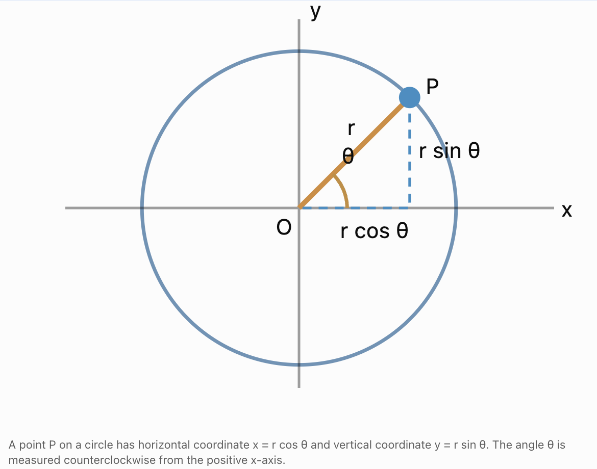
Trigonometric functions can describe the position of an object moving around a circle.
Consider an object moving around a circle of radius r, centred at the origin.
If its angular position is θ, its Cartesian coordinates are:
x = r cos θ
y = r sin θ
These equations follow directly from right-triangle trigonometry.
Circular Motion with Time
For constant angular velocity:
θ = ωt + φ
where φ is the initial angle.
Substituting:
x(t) = r cos(ωt + φ)
y(t) = r sin(ωt + φ)
These equations describe the horizontal and vertical positions of a point moving in uniform circular motion.
Worked Example: Position on a Rotating Wheel
A wheel has a radius of 2 m.
A point on the rim is located at an angle of 60° above the positive horizontal axis.
Find its horizontal and vertical coordinates relative to the centre.
Horizontal Position
x = r cos θ
= 2 cos 60°
= 2 × 0.5
x = 1.0 m
Vertical Position
y = r sin θ
= 2 sin 60°
= 2 × √3/2
y = √3 m ≈ 1.73 m
Interpretation
The point is 1.0 m to the right and approximately 1.73 m above the centre.
Rotational Motion and Sinusoidal Graphs
The horizontal and vertical coordinates of a rotating point vary sinusoidally with time.
For uniform circular motion:
x(t) = r cos(ωt + φ)
y(t) = r sin(ωt + φ)
These functions have:
-
Amplitude = r.
-
Period = 2π/|ω|.
-
Frequency = |ω|/(2π).
Graphical Interpretation
The horizontal position follows a cosine curve.
The vertical position follows a sine curve.
The two oscillations differ in phase by π/2 radians, or 90°.
This explains why circular motion is closely connected to simple harmonic motion.
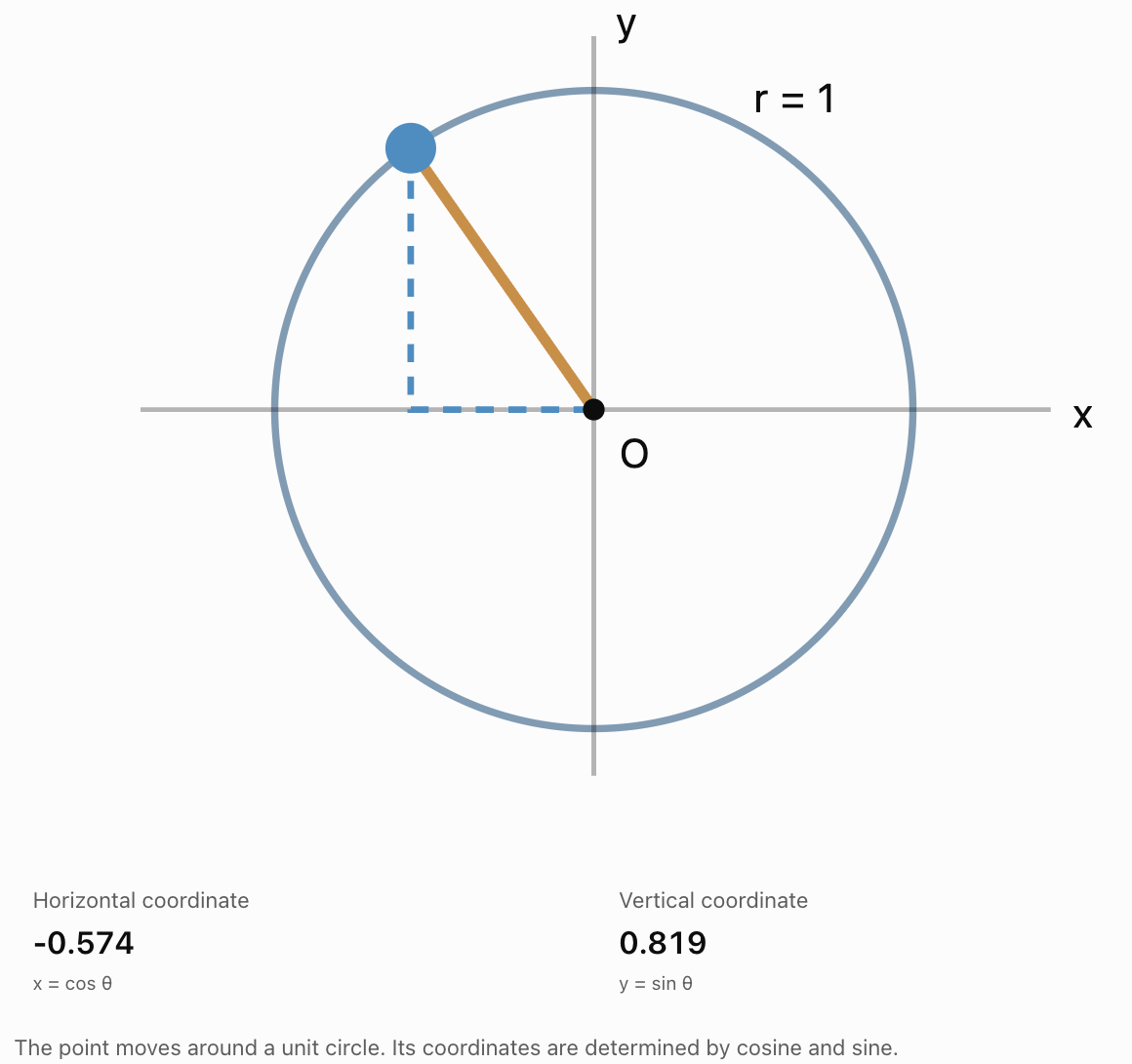
Interactive Rotational Motion Model
Adjust the angle to see how the horizontal and vertical coordinates change.
Velocity Components in Circular Motion
The velocity of an object moving in a circle is tangent to the circular path.
For counterclockwise uniform circular motion:
x(t) = r cos(ωt + φ)
y(t) = r sin(ωt + φ)
Differentiating with respect to time gives:
vₓ = −rω sin(ωt + φ)
vᵧ = rω cos(ωt + φ)
The magnitude of the velocity is:
v = √(vₓ² + vᵧ²)
Substituting:
v = r|ω|√(sin²θ + cos²θ)
Since:
sin²θ + cos²θ = 1
then:
v = r|ω|
Important Observation
The speed remains constant in uniform circular motion, but the direction of velocity changes continuously.
Therefore, the object is accelerating.
Centripetal Acceleration
An object moving in a circular path experiences acceleration directed toward the centre.
This is called centripetal acceleration.
Its magnitude is:
a_c = v²/r
Using v = r|ω|:
a_c = rω²
where:
-
a_c = centripetal acceleration.
-
v = tangential speed.
-
r = radius.
-
ω = angular velocity.
Worked Example
A car travels around a circular track of radius 50 m at a constant speed of 20 m/s.
Calculate its centripetal acceleration.
a_c = v²/r
= 20²/50
= 400/50
a_c = 8.0 m/s²
Interpretation
The car experiences an acceleration of 8.0 m/s² toward the centre of the circular track.
Even though its speed is constant, its velocity changes because its direction changes.

Centripetal Force
Newton's Second Law states:
F_net = ma
For circular motion, the net inward force is:
F_c = mv²/r
or:
F_c = mrω²
This inward net force is called the centripetal force.
Important Distinction
Centripetal force is not a separate type of physical force.
It is the name given to the resultant force directed toward the centre of a circular path.
It may be provided by:
-
Friction.
-
Tension.
-
Gravity.
-
Normal force.
-
A combination of forces.
Worked Example
A 2 kg object moves in a circle of radius 1.5 m at a speed of 6 m/s.
Calculate the required centripetal force.
F_c = mv²/r
= 2 × 6²/1.5
= 72/1.5
F_c = 48 N
The net inward force must be 48 N.
Angular Acceleration
Angular velocity may change over time.
Angular acceleration is the rate of change of angular velocity.
Average angular acceleration is:
α_avg = Δω/Δt
where:
-
α = angular acceleration in rad/s².
-
Δω = change in angular velocity.
-
Δt = time interval.
Worked Example
A motor increases its angular velocity from 10 rad/s to 50 rad/s in eight seconds.
Calculate its average angular acceleration.
α = (50 − 10)/8
= 40/8
α = 5 rad/s²
Interpretation
The motor's angular velocity increases by 5 rad/s every second on average.
Equations of Rotational Kinematics
For constant angular acceleration, rotational motion follows equations similar to linear kinematics.
|
Linear motion |
Rotational motion |
|---|---|
|
v = u + at |
ω = ω₀ + αt |
|
s = ut + 1/2 at² |
Δθ = ω₀t + 1/2 αt² |
|
v² = u² + 2as |
ω² = ω₀² + 2αΔθ |
|
s = (u + v)t/2 |
Δθ = (ω₀ + ω)t/2 |
where:
-
ω₀ = initial angular velocity.
-
ω = final angular velocity.
-
α = constant angular acceleration.
-
Δθ = angular displacement.
-
t = time.
These equations are useful for rotating systems that speed up or slow down uniformly.
Worked Example: Accelerating Wheel
A wheel starts from rest and accelerates uniformly at 4 rad/s² for five seconds.
Calculate its final angular velocity and angular displacement.
Final Angular Velocity
ω = ω₀ + αt
= 0 + 4 × 5
ω = 20 rad/s
Angular Displacement
Δθ = ω₀t + 1/2 αt²
= 0 + 1/2 × 4 × 5²
= 2 × 25
Δθ = 50 rad
Number of Revolutions
N = Δθ/(2π)
= 50/(2π)
N ≈ 7.96 revolutions
The wheel completes approximately 7.96 revolutions while accelerating.
Tangential and Radial Acceleration
When angular velocity changes, a rotating point may experience two perpendicular acceleration components.
Tangential Acceleration
Tangential acceleration changes the speed.
a_t = rα
Radial Acceleration
Radial or centripetal acceleration changes the direction of velocity.
a_c = rω²
Total Acceleration
Since the two components are perpendicular:
a_total = √(a_t² + a_c²)
Worked Example
A rotating disk has:
r = 0.40 m
ω = 6 rad/s
α = 3 rad/s²
Tangential acceleration:
a_t = 0.40 × 3
a_t = 1.2 m/s²
Centripetal acceleration:
a_c = 0.40 × 6²
a_c = 14.4 m/s²
Total acceleration:
a_total = √(1.2² + 14.4²)
a_total ≈ 14.45 m/s²
The acceleration is dominated by the centripetal component.
Torque and Rotational Forces
Torque is the turning effect of a force about an axis.
The magnitude of torque is:
τ = rF sin θ
where:
-
τ = torque in newton-metres (N·m).
-
r = distance from the axis to the point where the force acts.
-
F = force magnitude.
-
θ = angle between the position vector and force.
Maximum Torque
Torque is greatest when the force acts perpendicular to the position vector.
When θ = 90°:
sin 90° = 1
Therefore:
τ_max = rF
Zero Torque
When the force acts directly toward or away from the axis:
θ = 0° or 180°
sin θ = 0
Therefore:
τ = 0
This explains why pushing directly toward a door hinge produces little turning effect.

Worked Example: Torque at an Angle
A mechanic applies a force of 80 N to a wrench.
The force is applied 0.30 m from the bolt at an angle of 60° to the wrench.
Calculate the torque magnitude.
τ = rF sin θ
= 0.30 × 80 × sin 60°
= 24 × 0.866
τ ≈ 20.8 N·m
Interpretation
The turning effect is approximately 20.8 N·m.
If the force were applied perpendicular to the wrench, the torque would be:
τ = 0.30 × 80
= 24 N·m
The perpendicular force produces greater torque.
Moment of Inertia
In linear motion, mass measures resistance to acceleration.
In rotational motion, moment of inertia measures resistance to angular acceleration about a particular axis.
It is represented by I.
For a collection of point masses:
I = Σmr²
where r is the perpendicular distance of each mass from the rotation axis.
Common Moments of Inertia
|
Object |
Moment of inertia about specified axis |
|---|---|
|
Point mass |
I = mr² |
|
Thin hoop, central perpendicular axis |
I = mr² |
|
Solid disk, central perpendicular axis |
I = 1/2 mr² |
|
Solid sphere, diameter |
I = 2/5 mr² |
|
Thin rod, axis through centre perpendicular to rod |
I = 1/12 mL² |
Important Principle
Mass located farther from the axis contributes more to moment of inertia.
This is why the distribution of mass matters in rotational mechanics.
Newton's Second Law for Rotation
For a rigid body rotating about a fixed axis:
τ_net = Iα
where:
-
τ_net = net external torque about the axis.
-
I = moment of inertia about that axis.
-
α = angular acceleration.
This is the rotational equivalent of:
F_net = ma
Worked Example
A solid disk has:
Mass = 4 kg
Radius = 0.50 m
A net torque of 2 N·m acts about its central axis.
Find its angular acceleration.
Step 1: Calculate Moment of Inertia
I = 1/2 mr²
= 1/2 × 4 × 0.50²
I = 0.50 kg·m²
Step 2: Calculate Angular Acceleration
α = τ_net/I
= 2/0.50
α = 4 rad/s²
The disk accelerates at 4 rad/s².
Rotational Kinetic Energy
A rotating object possesses kinetic energy.
The rotational kinetic energy is:
E_rot = 1/2 Iω²
Worked Example
A flywheel has a moment of inertia of 3 kg·m² and rotates at 10 rad/s.
Calculate its rotational kinetic energy.
E_rot = 1/2 × 3 × 10²
= 1.5 × 100
E_rot = 150 J
Engineering Applications
Rotational kinetic energy is important in:
-
Flywheels.
-
Vehicle wheels.
-
Turbines.
-
Rotating motors.
-
Energy-storage systems.

Angular Momentum
Angular momentum describes the rotational motion of a body.
For a rigid body rotating about a fixed principal axis:
L = Iω
where:
-
L = angular momentum.
-
I = moment of inertia.
-
ω = angular velocity.
If the net external torque is zero, angular momentum is conserved.
I₁ω₁ = I₂ω₂
Example: Figure Skater
A figure skater spins with arms extended.
When the skater pulls their arms inward, the moment of inertia decreases.
If external torque is negligible, angular velocity increases to conserve angular momentum.
This explains why a skater spins faster when pulling their arms close to the body.

Rolling Motion
A wheel rolling without slipping combines translational and rotational motion.
For pure rolling:
v = rω
where v is the speed of the wheel's centre.
For acceleration:
a = rα
These relationships apply when there is no slipping between the wheel and the surface.
Worked Example
A bicycle wheel has a radius of 0.35 m.
The bicycle moves at 7 m/s without slipping.
Calculate the wheel's angular velocity.
ω = v/r
= 7/0.35
ω = 20 rad/s
Number of Revolutions
The wheel's circumference is:
C = 2πr
= 2π × 0.35
≈ 2.20 m
If the bicycle travels 100 m:
N = 100/(2π × 0.35)
N ≈ 45.5 revolutions
Gear Ratios
Gears transfer rotational motion and torque between connected shafts.
For two meshing gears with no slipping at the contact point, the tangential speeds are equal.
r₁|ω₁| = r₂|ω₂|
Therefore:
|ω₂|/|ω₁| = r₁/r₂
For gears with the same tooth spacing, the ratio can also be expressed using the numbers of teeth.
|ω₂|/|ω₁| = N₁/N₂
where N₁ and N₂ are the tooth counts.
Worked Example
Gear A has 20 teeth and rotates at 600 rpm.
Gear B has 60 teeth.
Calculate Gear B's rotational speed.
ω_B = 600 × 20/60
= 200 rpm
Interpretation
The larger gear rotates more slowly.
For ideal gears, the reduction in angular speed corresponds to an increase in available torque.
Two externally meshing gears rotate in opposite directions.

Engineering Application: Ferris Wheel Motion
A Ferris wheel provides an example of circular motion modelled using trigonometry.
Suppose a Ferris wheel has:
-
Radius = 15 m.
-
Centre height = 18 m.
-
Period = 60 s.
A passenger begins at the lowest point.
Step 1: Determine Angular Velocity
ω = 2π/T
= 2π/60
ω = π/30 rad/s
Step 2: Construct the Height Function
Because the passenger starts at the bottom:
h(t) = 18 − 15 cos(πt/30)
where h is measured in metres.
Step 3: Calculate the Starting Height
At t = 0:
h(0) = 18 − 15 cos 0
= 18 − 15
h(0) = 3 m
Step 4: Calculate Height After 15 Seconds
h(15) = 18 − 15 cos(π/2)
= 18 − 0
h(15) = 18 m
Step 5: Calculate Height After 30 Seconds
h(30) = 18 − 15 cos π
= 18 + 15
h(30) = 33 m
Interpretation
The passenger begins 3 m above the ground, reaches the centre height after 15 seconds, and reaches the highest point after 30 seconds.
The model repeats every 60 seconds.
Graphing Periodic Rotational Motion
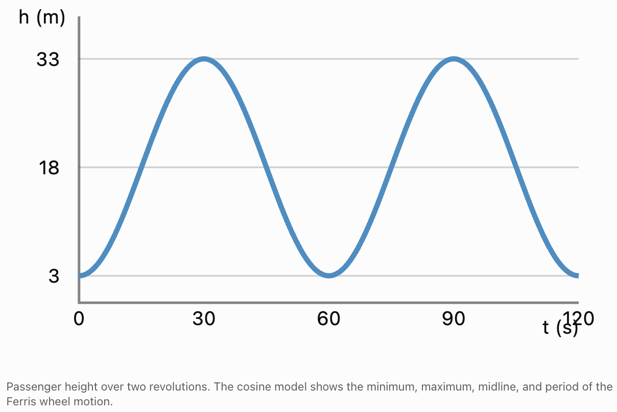
The Ferris wheel height model is:
h(t) = 18 − 15 cos(πt/30)
Its important features are:
- Midline = 18 m.
- Amplitude = 15 m.
- Period = 60 s.
- Minimum height = 3 m.
- Maximum height = 33 m.
Interpreting Rotational Motion Graphs
Rotational motion can be represented using several types of graphs.
Angular Displacement–Time Graph
The gradient represents angular velocity.
For constant angular velocity, the graph is a straight line.
Angular Velocity–Time Graph
The gradient represents angular acceleration.
The signed area under the graph represents angular displacement.
Angular Acceleration–Time Graph
The signed area under the graph represents the change in angular velocity.
Sinusoidal Position–Time Graph
The graph of a rotating point's horizontal or vertical coordinate is sinusoidal during uniform circular motion.
Its amplitude corresponds to the radius, while its period corresponds to the time for one revolution.
Practical Application: Wind Turbines
Wind turbines convert energy from moving air into rotational mechanical energy and then electrical energy.
Suppose a wind turbine blade extends 40 m from the rotation axis and rotates at 15 rpm.
Angular Velocity
f = 15/60
= 0.25 Hz
ω = 2π × 0.25
ω ≈ 1.57 rad/s
Blade-Tip Speed
v = rω
= 40 × 1.57
v ≈ 62.8 m/s
Interpretation
Although the turbine completes only 15 revolutions per minute, the blade tip moves at approximately 62.8 m/s.
This demonstrates why engineers must consider radius as well as angular velocity when analysing rotating machinery.
Practical Application: Vehicle Wheels
Vehicle wheels convert rotational motion into forward motion.
For rolling without slipping:
v = rω
A vehicle travelling at 25 m/s has wheels with radius 0.32 m.
Angular velocity:
ω = 25/0.32
ω ≈ 78.13 rad/s
Convert to rpm:
rpm = ω × 60/(2π)
rpm ≈ 746
The wheels rotate approximately 746 times per minute.
Practical Application: Robotic Arms
Robotic arms often contain rotating joints.
The position of the end of a single rigid arm of length L can be described using:
x = L cos θ
y = L sin θ
For a two-link robotic arm operating in a plane:
x = L₁ cos θ₁ + L₂ cos(θ₁ + θ₂)
y = L₁ sin θ₁ + L₂ sin(θ₁ + θ₂)
where:
-
L₁ and L₂ are the lengths of the arm segments.
-
θ₁ is the angle of the first segment.
-
θ₂ is the angle of the second segment relative to the first.
These equations are examples of forward kinematics.
They allow engineers to calculate the position of a robotic tool from the joint angles.

Common Mistakes
Using degrees in equations that require radians
Rotational mechanics formulas such as s = rθ and v = rω require angles in radians.
Confusing angular velocity with tangential speed
Angular velocity is measured in rad/s, while tangential speed is measured in m/s.
Assuming all points on a rotating disk have the same linear speed
Points farther from the axis move faster.
Confusing angular displacement with the number of revolutions
One revolution equals 2π radians.
Assuming constant speed means zero acceleration
Uniform circular motion involves centripetal acceleration because velocity changes direction.
Treating centripetal force as an additional physical force
Centripetal force is the net inward force supplied by real forces.
Confusing tangential and centripetal acceleration
Tangential acceleration changes speed, while centripetal acceleration changes velocity direction.
Using the wrong angle in torque calculations
The torque formula uses the angle between the position vector and applied force.
Ignoring the distribution of mass
Moment of inertia depends on both mass and its distance from the rotation axis.
Assuming all rotational motion has constant angular acceleration
The standard rotational kinematics equations require constant angular acceleration.
Ignoring the direction of rotation
Clockwise and counterclockwise motion have opposite signs under the usual convention.
Applying rolling equations when slipping occurs
The relationship v = rω for a wheel's centre requires rolling without slipping.
Key Terms
-
Rotational Motion: Motion involving an object turning around an axis.
-
Circular Motion: Motion along a circular path.
-
Axis of Rotation: The line about which an object rotates.
-
Radius: The distance from the centre or axis to a point on a circular path.
-
Radian: An angular unit defined by the ratio of arc length to radius.
-
Angular Position: The orientation of a rotating object relative to a reference direction.
-
Angular Displacement: The change in angular position.
-
Arc Length: The distance measured along a circular path.
-
Angular Velocity: The rate of change of angular displacement.
-
Angular Speed: The magnitude of angular velocity.
-
Angular Acceleration: The rate of change of angular velocity.
-
Tangential Velocity: The linear velocity of an object moving along a circular path.
-
Tangential Acceleration: Acceleration that changes the magnitude of tangential velocity.
-
Centripetal Acceleration: Acceleration directed toward the centre of a circular path.
-
Centripetal Force: The net inward force required for circular motion.
-
Uniform Circular Motion: Circular motion with constant speed.
-
Period: The time required for one complete revolution.
-
Frequency: The number of revolutions or cycles per second.
-
Revolutions per Minute (rpm): The number of complete rotations in one minute.
-
Sinusoidal Function: A function described by sine or cosine.
-
Amplitude: The maximum displacement from a sinusoidal function's midline.
-
Phase Angle: An angular quantity describing position within a repeating cycle.
-
Torque: The turning effect of a force about an axis.
-
Moment Arm: The perpendicular distance from an axis to a force's line of action.
-
Moment of Inertia: A measure of resistance to angular acceleration about an axis.
-
Rotational Kinetic Energy: Energy associated with rotational motion.
-
Angular Momentum: A quantity describing rotational motion that is conserved when net external torque is zero.
-
Rolling Without Slipping: Motion in which a rolling object's contact point is instantaneously at rest relative to the surface.
-
Gear Ratio: A relationship between the rotational speeds or tooth counts of connected gears.
-
Forward Kinematics: Calculating the position and orientation of a mechanism from its joint coordinates.
-
Periodic Motion: Motion that repeats at regular time intervals.
Key Takeaways
-
Trigonometry provides a mathematical foundation for analysing circular and rotational motion.
-
Angular displacement measures the angle through which an object rotates.
-
Radians are the standard angular units used in rotational mechanics.
-
Arc length and angular displacement are related by s = rθ.
-
Angular velocity measures the rate of change of angular position.
-
Frequency, period, and angular velocity are related by ω = 2πf = 2π/T for uniform circular motion.
-
Tangential speed depends on radius and angular velocity.
-
The position of a point moving in a circle can be modelled using sine and cosine functions.
-
Horizontal and vertical circular-motion coordinates vary sinusoidally with time.
-
Uniform circular motion involves centripetal acceleration even when speed remains constant.
-
Centripetal acceleration is directed toward the centre of the circular path.
-
Centripetal force is the net inward force required to maintain circular motion.
-
Angular acceleration describes changes in angular velocity.
-
Constant-angular-acceleration equations are analogous to linear kinematics equations.
-
Torque depends on force, distance from the axis, and the angle of application.
-
Moment of inertia depends on how mass is distributed relative to the rotation axis.
-
Newton's Second Law for fixed-axis rotation is τ_net = Iα.
-
Rotating objects possess rotational kinetic energy.
-
Angular momentum is conserved when net external torque is zero.
-
Rolling motion connects translational and rotational quantities.
-
Gear systems use rotational relationships to change angular speed and torque.
-
Ferris wheels, turbines, vehicle wheels, and robotic arms can all be analysed using trigonometric models.
Check Your Understanding
Recall and Understanding
-
Explain the difference between circular motion and rotational motion.
-
Define angular displacement, angular velocity, and angular acceleration.
-
Explain why radians are used in rotational mechanics.
-
Describe the relationship between angular velocity and tangential speed.
-
Explain why an object moving in a circle at constant speed still experiences acceleration.
Application
-
A wheel rotates through 720°. Calculate its angular displacement in radians.
-
A motor rotates at 2,400 rpm. Calculate its frequency in hertz and angular velocity in rad/s.
-
A wheel with radius 0.45 m rotates at 12 rad/s. Calculate the tangential speed of a point on its rim.
-
A 3 kg object moves in a circular path of radius 2 m at a speed of 8 m/s. Calculate its centripetal acceleration and the required centripetal force.
-
A force of 120 N is applied to a wrench 0.25 m from the rotation axis at an angle of 45°. Calculate the torque magnitude.
Analysis and Challenge
-
A disk starts from rest and accelerates uniformly at 6 rad/s² for eight seconds. Calculate its final angular velocity, angular displacement, and number of revolutions.
-
A Ferris wheel has a radius of 12 m and its centre is 15 m above the ground. It completes one revolution every 40 seconds. A passenger begins at the lowest point. Construct a trigonometric model for the passenger's height and calculate the height after 10, 20, and 30 seconds.
-
A solid disk has a mass of 5 kg and a radius of 0.40 m. A net torque of 4 N·m acts about its central axis. Calculate its moment of inertia and angular acceleration.
-
Two meshing gears have 24 and 72 teeth. The smaller gear rotates at 900 rpm. Calculate the rotational speed of the larger gear and explain how the gear arrangement affects speed and torque.
-
A robotic arm consists of two segments with lengths 1.5 m and 1.0 m. The first segment is positioned at 30° above the horizontal, and the second segment is rotated a further 45° relative to the first. Calculate the horizontal and vertical coordinates of the end of the robotic arm.
Final Summary
Rotational motion connects geometry, trigonometry, mechanics, and engineering.
Angular displacement, angular velocity, and angular acceleration describe how objects rotate, while radians provide a natural mathematical measure of angular motion.
Sine and cosine functions allow the position of a rotating point to be expressed in terms of time and angle.
Tangential velocity connects rotational motion to linear motion, while centripetal acceleration explains why objects moving in circles experience acceleration even when their speed is constant.
Torque, moment of inertia, and angular momentum extend rotational analysis to forces, energy, and the dynamics of rigid bodies.
These principles have practical applications in motors, turbines, wheels, gears, robotic arms, and many other engineering systems.
The central principle is that trigonometry allows rotational motion to be represented mathematically, while the laws of mechanics explain how forces and energy determine the behaviour of rotating systems.
3. Vector Applications
Learning outcomes
- I can resolve vectors using trigonometry.
- I can analyse vector quantities geometrically.
- I can solve navigation problems.
- I can apply trigonometry to force systems.
- I can connect vectors with trigonometric methods.
Vector Applications
Introduction to Vector Applications
Vectors are mathematical quantities that have both magnitude and direction. They are essential in physics, engineering, navigation, robotics, and many other areas of mathematics and science.
Trigonometry provides powerful methods for working with vectors because it allows us to calculate their horizontal and vertical components, combine vectors, and determine unknown magnitudes and directions.
For example, trigonometry can help answer questions such as:
-
How can a force acting at an angle be separated into horizontal and vertical components?
-
How far north and east has an aircraft travelled?
-
What is the resultant force when several forces act on an object?
-
How can the direction of a displacement be calculated?
-
How does wind affect the motion of an aircraft?
-
How can vectors be used to analyse structures and mechanical systems?
Vector methods allow us to replace complicated directional problems with manageable mathematical calculations.


Scalars and Vectors
Physical quantities can be classified as scalars or vectors.
Scalar Quantities
A scalar has magnitude only.
Examples include:
-
Mass.
-
Time.
-
Temperature.
-
Distance.
-
Speed.
-
Energy.
A scalar can be described completely using a numerical value and an appropriate unit.
Vector Quantities
A vector has both magnitude and direction.
Examples include:
-
Displacement.
-
Velocity.
-
Acceleration.
-
Force.
-
Momentum.
-
Weight.
For example:
A speed of 20 m/s is a scalar.
A velocity of 20 m/s east is a vector.
Comparison
|
Scalar |
Vector |
|---|---|
|
Magnitude only |
Magnitude and direction |
|
Added using ordinary arithmetic |
Added using vector methods |
|
Example: 5 km |
Example: 5 km north |
|
Example: 10 m/s speed |
Example: 10 m/s east velocity |
|
Example: 50 N is a force magnitude |
Example: 50 N upward is a force vector |
Representing Vectors
Vectors are commonly represented using arrows.
The length of the arrow represents magnitude.
The direction of the arrow represents the direction of the vector.
A vector may be represented using a capital letter, such as A, B, or R.
Its magnitude is written:
|A|
Here, A represents the vector, while |A| represents its magnitude.
This notation avoids the unusual combining characters that sometimes display incorrectly when copied into Moodle.
Example
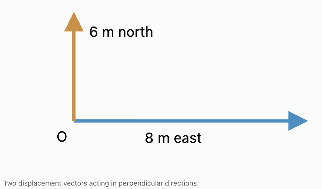
A displacement of 8 m east can be represented by an arrow pointing to the right.
A displacement of 6 m north can be represented by an arrow pointing upward.
When vectors are drawn to scale, their lengths are proportional to their magnitudes.
Cartesian Components of Vectors
A vector in two dimensions can be separated into two perpendicular components.
These are usually:
-
Horizontal component, Aₓ.
-
Vertical component, Aᵧ.
The components describe how much of the vector acts in each direction.
Resolving a Vector
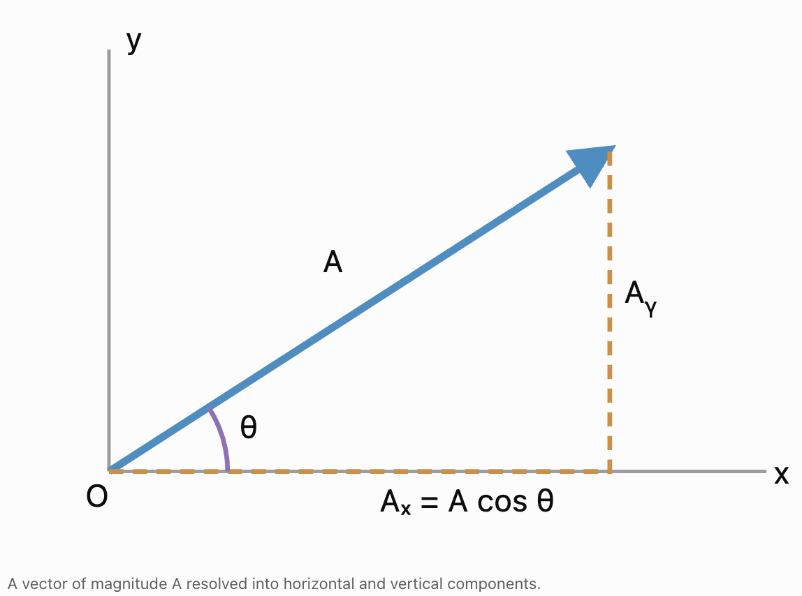
Suppose a vector has magnitude A and makes an angle θ with the positive x-axis.
Its components are:
Aₓ = A cos θ
Aᵧ = A sin θ
These equations come from right-triangle trigonometry.
Why Cosine and Sine?
For a right triangle:
cos θ = Adjacent/Hypotenuse
sin θ = Opposite/Hypotenuse
The vector magnitude is the hypotenuse.
The horizontal component is adjacent to θ.
The vertical component is opposite θ.
Therefore:
Aₓ = A cos θ
Aᵧ = A sin θ
Visualizing Vector Resolution
Worked Example: Resolving a Displacement Vector
A student walks 20 m at an angle of 30° north of east.
Calculate the horizontal and vertical components of the displacement.
Step 1: Identify the Information
Magnitude:
A = 20 m
Angle:
θ = 30°
Step 2: Calculate the Horizontal Component
Aₓ = A cos θ
= 20 cos 30°
= 20 × 0.866
Aₓ ≈ 17.32 m east
Step 3: Calculate the Vertical Component
Aᵧ = A sin θ
= 20 sin 30°
= 20 × 0.5
Aᵧ = 10.0 m north
Interpretation
The displacement is equivalent to travelling approximately 17.32 m east and 10.0 m north.
These perpendicular components combine to produce the original 20 m displacement.
Vector Components in Different Quadrants
The signs of vector components depend on direction.
Using the standard Cartesian coordinate system:
|
Quadrant |
Horizontal component |
Vertical component |
|---|---|---|
|
I |
Positive |
Positive |
|
II |
Negative |
Positive |
|
III |
Negative |
Negative |
|
IV |
Positive |
Negative |
Example
A vector of magnitude 15 N acts at 150° counterclockwise from the positive x-axis.
Horizontal component:
Fₓ = 15 cos 150°
Fₓ ≈ −12.99 N
Vertical component:
Fᵧ = 15 sin 150°
Fᵧ = 7.50 N
The force acts to the left and upward.
Important Principle
A negative component does not mean the vector has a negative magnitude.
It indicates direction relative to the chosen coordinate axes.
Calculating Vector Magnitude from Components
If the horizontal and vertical components are known, the magnitude can be calculated using the Pythagorean theorem.
|A| = √(Aₓ² + Aᵧ²)
Worked Example
A displacement vector has components:
Aₓ = 12 m
Aᵧ = 5 m
Calculate the magnitude.
|A| = √(12² + 5²)
= √(144 + 25)
= √169
|A| = 13 m
Calculating Vector Direction
The direction of a vector can be found using the tangent ratio.
tan θ = Aᵧ/Aₓ
Therefore:
θ = tan⁻¹(Aᵧ/Aₓ)
However, the signs of the components must be considered to identify the correct quadrant.
A calculator's inverse tangent may return an angle that does not directly represent the required direction.
Worked Example
A vector has components:
Aₓ = 8 m
Aᵧ = 6 m
Calculate its direction.
tan θ = 6/8
= 0.75
θ = tan⁻¹(0.75)
θ ≈ 36.87°
Both components are positive, so the vector lies in Quadrant I.
The direction is:
36.87° north of east
Calculator Note
When available, the function atan2(Aᵧ,Aₓ) is useful because it accounts for the signs of both components.
Adding Vectors Geometrically
Vectors can be added using the head-to-tail method.
To add vectors A and B:
-
Draw A.
-
Place the tail of B at the head of A.
-
Draw the resultant from the tail of A to the head of B.
The resultant vector is:
R = A + B
Example
A person walks:
8 m east
followed by:
6 m north
The resultant displacement is the diagonal of a right triangle.
Magnitude:
R = √(8² + 6²)
= √100
R = 10 m
Direction:
θ = tan⁻¹(6/8)
θ ≈ 36.87° north of east
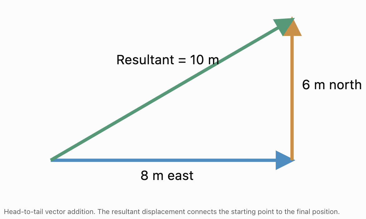
Adding Vectors Using Components
When several vectors act at different angles, resolving them into components is often the most efficient method.
For multiple vectors:
Rₓ = ΣAₓ
Rᵧ = ΣAᵧ
Then:
R = √(Rₓ² + Rᵧ²)
The direction can be calculated using:
θ = tan⁻¹(Rᵧ/Rₓ)
with the appropriate quadrant adjustment.
General Procedure
-
Choose positive x- and y-directions.
-
Resolve every vector into components.
-
Add the horizontal components.
-
Add the vertical components.
-
Calculate the resultant magnitude.
-
Calculate the direction.
-
Interpret the result in context.
Worked Example: Three Forces Acting on an Object
Three forces act on an object:
-
F₁ = 20 N east.
-
F₂ = 15 N north.
-
F₃ = 10 N west.
Calculate the resultant force.
Step 1: Resolve Horizontal Forces
Take east as positive.
F₁ₓ = +20 N
F₃ₓ = −10 N
Total horizontal force:
Rₓ = 20 − 10
Rₓ = 10 N
Step 2: Resolve Vertical Forces
F₂ᵧ = +15 N
Therefore:
Rᵧ = 15 N
Step 3: Calculate Magnitude
R = √(10² + 15²)
= √325
R ≈ 18.03 N
Step 4: Calculate Direction
θ = tan⁻¹(15/10)
θ ≈ 56.31°
Final Answer
Resultant force ≈ 18.03 N at 56.31° north of east.
Worked Example: Forces at Different Angles
Three forces act on an object:
-
F₁ = 50 N at 30° above the positive x-axis.
-
F₂ = 40 N at 120° counterclockwise from the positive x-axis.
-
F₃ = 30 N directly downward.
Find the resultant force.
Step 1: Resolve F₁
F₁ₓ = 50 cos 30°
F₁ₓ ≈ 43.30 N
F₁ᵧ = 50 sin 30°
F₁ᵧ = 25.00 N
Step 2: Resolve F₂
F₂ₓ = 40 cos 120°
F₂ₓ = −20.00 N
F₂ᵧ = 40 sin 120°
F₂ᵧ ≈ 34.64 N
Step 3: Resolve F₃
F₃ₓ = 0 N
F₃ᵧ = −30 N
Step 4: Add Components
Rₓ = 43.30 − 20.00 + 0
Rₓ ≈ 23.30 N
Rᵧ = 25.00 + 34.64 − 30.00
Rᵧ ≈ 29.64 N
Step 5: Calculate Magnitude
R = √(23.30² + 29.64²)
R ≈ 37.70 N
Step 6: Calculate Direction
θ = tan⁻¹(29.64/23.30)
θ ≈ 51.8°
Final Answer
The resultant force is approximately 37.70 N at 51.8° above the positive x-axis.
Vector Subtraction
Vector subtraction can be interpreted as adding the opposite vector.
A − B = A + (−B)
The opposite vector has the same magnitude but points in the opposite direction.
Example
A = (8, 5)
B = (3, 7)
Subtract the components:
A − B = (8 − 3, 5 − 7)
A − B = (5, −2)
Magnitude:
|A − B| = √(5² + (−2)²)
= √29
≈ 5.39 units
The resultant points right and downward.
Navigation Using Vectors
Navigation problems frequently involve displacement, velocity, and direction.
A common navigation convention uses bearings.
A bearing is measured clockwise from north.
Examples include:
-
North = 000°.
-
East = 090°.
-
South = 180°.
-
West = 270°.
For a displacement of magnitude d and bearing β:
Eastward component = d sin β
Northward component = d cos β
These formulas differ from the standard x-axis convention because bearings are measured from north rather than east.

Worked Example: Navigation with Bearings
A boat travels 12 km on a bearing of 060°.
Calculate its eastward and northward displacements.
Eastward Component
E = 12 sin 60°
= 12 × 0.866
E ≈ 10.39 km
Northward Component
N = 12 cos 60°
= 12 × 0.5
N = 6.00 km
Interpretation
The boat travels approximately 10.39 km east and 6.00 km north.
Multi-Stage Navigation Problems
A ship travels:
-
20 km east.
-
15 km north.
-
10 km west.
Find its resultant displacement.
Horizontal Displacement
E = 20 − 10
E = 10 km
Vertical Displacement
N = 15 km
Magnitude
R = √(10² + 15²)
R ≈ 18.03 km
Bearing
The angle east of north is:
β = tan⁻¹(10/15)
β ≈ 33.69°
Final Answer
Resultant displacement ≈ 18.03 km on a bearing of 034°.
Aircraft Navigation and Wind Velocity
Aircraft navigation provides an important example of vector addition.
An aircraft's velocity relative to the ground is the sum of:
-
Aircraft velocity relative to the air.
-
Wind velocity relative to the ground.
v_ground = v_aircraft + v_wind
Here, each symbol represents a vector quantity.
Worked Example
An aircraft flies due north at 200 km/h relative to the air.
A wind blows due east at 50 km/h.
Calculate the aircraft's ground speed and direction.
Step 1: Identify Components
Eastward velocity:
vₓ = 50 km/h
Northward velocity:
vᵧ = 200 km/h
Step 2: Calculate Ground Speed
v = √(50² + 200²)
= √42,500
v ≈ 206.16 km/h
Step 3: Calculate Direction
Angle east of north:
θ = tan⁻¹(50/200)
θ ≈ 14.04°
Final Answer
The aircraft travels at approximately:
206.16 km/h on a bearing of 014°.
Interpretation
The wind causes the aircraft to drift east of its intended northerly direction.

River Crossing Problems
A boat crossing a river experiences two velocity components:
-
Velocity relative to the water.
-
River current velocity.
Worked Example
A boat moves north across a river at 4 m/s relative to the water.
The river current flows east at 3 m/s.
Calculate the boat's resultant velocity.
Magnitude
v = √(4² + 3²)
v = 5 m/s
Direction
θ = tan⁻¹(3/4)
θ ≈ 36.87° east of north
Interpretation
The boat travels diagonally downstream rather than directly across the river.
If the river is 120 m wide, the crossing time is:
t = 120/4
t = 30 s
The downstream drift is:
d = 3 × 30
d = 90 m
The boat lands 90 m downstream from the point directly opposite its starting position.
Force Equilibrium
An object is in translational equilibrium when the resultant force is zero.
ΣFₓ = 0
ΣFᵧ = 0
This means the object has zero acceleration.
It may be stationary or moving at constant velocity.
Example: Hanging Sign
A sign is supported by two identical cables.
Each cable makes an angle of 30° above the horizontal.
The sign has a weight of 200 N.
Find the tension in each cable.
Step 1: Identify Vertical Components
Each cable provides an upward component:
T sin 30°
The two vertical components balance the weight.
2T sin 30° = 200
Step 2: Solve
2T × 0.5 = 200
T = 200
T = 200 N
Interpretation
Each cable has a tension of 200 N.
The horizontal components cancel because the cables are symmetrical.

Forces on an Inclined Plane
Vectors are especially useful for analysing forces on sloping surfaces.
Consider an object of mass m resting on an incline at angle θ.
Its weight is:
W = mg
The weight can be resolved into components:
Parallel to the slope:
W_parallel = mg sin θ
Perpendicular to the slope:
W_perpendicular = mg cos θ
Worked Example
A 10 kg box rests on a frictionless slope inclined at 25°.
Take:
g = 9.81 m/s²
Weight
W = 10 × 9.81
W = 98.1 N
Parallel Component
W_parallel = 98.1 sin 25°
≈ 41.46 N
Perpendicular Component
W_perpendicular = 98.1 cos 25°
≈ 88.91 N
Interpretation
The component of weight acting down the slope is approximately 41.46 N.
The perpendicular component is approximately 88.91 N.
If the box remains in contact with the frictionless slope and there is no acceleration perpendicular to it, the normal force is 88.91 N.

Resultant of Two Vectors Using the Cosine Rule
When two vectors are not perpendicular, the cosine rule can be used.
If vectors A and B have magnitudes A and B and an angle θ between them, the magnitude of their sum is:
R = √(A² + B² + 2AB cos θ)
Worked Example
Two forces act on an object:
F₁ = 40 N
F₂ = 30 N
The angle between them is 60°.
Calculate the resultant magnitude.
R = √(40² + 30² + 2 × 40 × 30 × cos 60°)
= √(1600 + 900 + 1200)
= √3700
R ≈ 60.83 N
Interpretation
The resultant is greater than either individual force but less than their combined magnitudes of 70 N.
The angle between the forces determines how strongly they reinforce each other.
Using the Sine Rule with Vectors
The sine rule can be used when a vector triangle contains known angles and side lengths.
For a triangle:
a/sin A = b/sin B = c/sin C
Example
Two displacement vectors form a triangle.
Suppose one side has length 12 km and is opposite an angle of 40°.
Another side is opposite an angle of 65°.
Find its length.
Using the sine rule:
b/sin 65° = 12/sin 40°
Therefore:
b = 12 sin 65°/sin 40°
b ≈ 16.92 km
This method is useful when vector directions are known but components are not the simplest approach.
Unit Vectors
A unit vector has magnitude 1.
In two-dimensional Cartesian coordinates:
-
i represents one unit in the positive x-direction.
-
j represents one unit in the positive y-direction.
Using unit-vector notation, a vector can be written:
A = Aₓi + Aᵧj
In this notation, i and j are unit vectors, not ordinary scalar variables.
Example
A force has components:
Fₓ = 12 N
Fᵧ = −5 N
In unit-vector form:
F = 12i − 5j N
Its magnitude is:
|F| = √(12² + (−5)²)
|F| = 13 N
Unit-vector notation makes vector addition straightforward.
Three-Dimensional Vectors
Vectors can also be represented in three dimensions.
A vector has components:
Aₓ, Aᵧ, A_z
Its magnitude is:
|A| = √(Aₓ² + Aᵧ² + A_z²)
Example
A displacement vector has components:
Aₓ = 3 m
Aᵧ = 4 m
A_z = 12 m
Magnitude:
|A| = √(3² + 4² + 12²)
= √169
|A| = 13 m
Applications
Three-dimensional vector calculations are important in:
-
Aircraft navigation.
-
Robotics.
-
Satellite motion.
-
Structural engineering.
-
Computer graphics.
-
Electromagnetic fields.
Dot Product and Trigonometry
The dot product connects vectors with the cosine of the angle between them.
For vectors A and B:
A · B = |A||B| cos θ
In component form:
A · B = AₓBₓ + AᵧBᵧ
For three-dimensional vectors, add A_zB_z.
Finding the Angle Between Vectors
Rearranging:
cos θ = (A · B)/(|A||B|)
Worked Example
A = (3, 4)
B = (5, 0)
Calculate the angle between the vectors.
Dot product:
A · B = 3 × 5 + 4 × 0
= 15
Magnitudes:
|A| = 5
|B| = 5
Therefore:
cos θ = 15/(5 × 5)
= 0.6
θ = cos⁻¹(0.6)
θ ≈ 53.13°
Work Done by a Force
The dot product has an important physical application in calculating work.
W = F · d
Therefore:
W = Fd cos θ
where:
-
W = work done.
-
F = force magnitude.
-
d = displacement magnitude.
-
θ = angle between force and displacement.
Worked Example
A person pulls a box with a force of 100 N at an angle of 30° above the horizontal.
The box moves 5 m horizontally.
Calculate the work done by the pulling force.
W = Fd cos θ
= 100 × 5 × cos 30°
= 500 × 0.866
W ≈ 433 J
Interpretation
Only the component of the force parallel to the displacement contributes to the work done.
The perpendicular component does no work during the horizontal displacement.
Vector Applications in Engineering
Vectors are essential for representing forces, velocities, accelerations, and displacements in engineering systems.
Structural Engineering
Engineers resolve forces to determine the loads acting on beams, cables, and supports.
Mechanical Engineering
Vectors describe the motion of machine components and the forces acting on them.
Aerospace Engineering
Aircraft motion depends on airspeed, wind velocity, thrust, lift, drag, and weight.
Civil Engineering
Vectors are used to analyse bridges, buildings, cranes, and other structures.
Robotics
Robotic systems use vector calculations to determine position, movement, and force.
Electrical Engineering
Alternating electrical quantities can be represented using phasors, which are rotating-vector representations of sinusoidal signals.


Choosing an Efficient Vector Method
Different vector problems require different strategies.
|
Problem type |
Recommended method |
|---|---|
|
Two perpendicular vectors |
Pythagorean theorem and tangent |
|
Vector with known magnitude and angle |
Sine and cosine components |
|
Several vectors at different angles |
Component method |
|
Two vectors with known included angle |
Cosine rule |
|
Vector triangle with known angles |
Sine rule |
|
Navigation with bearings |
North–east components |
|
Forces in equilibrium |
ΣFₓ = 0 and ΣFᵧ = 0 |
|
Work done by angled force |
Dot product |
|
Three-dimensional displacement |
3D component magnitude |
|
Angle between two vectors |
Dot product and inverse cosine |
The component method is often the most flexible because it can handle many vectors simultaneously.
Common Mistakes
Confusing scalar and vector quantities
Vectors require both magnitude and direction.
Using sine and cosine incorrectly
The correct formula depends on which axis the angle is measured from.
Ignoring negative components
Negative signs indicate direction and must be included when adding vectors.
Confusing magnitude with components
A vector's magnitude is not generally equal to either component.
Adding vector magnitudes directly
Magnitudes can only be added directly when the vectors act in the same direction.
Ignoring quadrant information
Inverse tangent calculations may require quadrant adjustments.
Confusing bearings with standard mathematical angles
Bearings are measured clockwise from north, while standard mathematical angles are measured counterclockwise from the positive x-axis.
Treating directional quantities as scalars
Forces, velocities, and displacements must be combined using vector methods.
Using the wrong angle in the cosine rule
The formula for the magnitude of a vector sum uses the angle between the two vectors.
Forgetting units
Force, velocity, and displacement have different units.
Ignoring physical context
A mathematically correct resultant must still be interpreted according to the real situation.
Key Terms
-
Scalar: A quantity with magnitude only.
-
Vector: A quantity with magnitude and direction.
-
Magnitude: The size or length of a vector.
-
Direction: The orientation in which a vector acts.
-
Displacement: A vector describing change in position.
-
Velocity: The rate of change of displacement.
-
Acceleration: The rate of change of velocity.
-
Force: A vector quantity describing an interaction capable of changing motion.
-
Vector Component: The contribution of a vector along a specified axis.
-
Horizontal Component: The component of a vector along the x-axis.
-
Vertical Component: The component of a vector along the y-axis.
-
Vector Resolution: Separating a vector into perpendicular components.
-
Resultant Vector: A single vector representing the sum of two or more vectors.
-
Vector Addition: Combining vectors to determine their resultant.
-
Vector Subtraction: Adding the opposite of a vector.
-
Head-to-Tail Method: A graphical method of vector addition.
-
Parallelogram Method: A graphical method for adding two vectors from a common starting point.
-
Cartesian Coordinates: A coordinate system using perpendicular axes.
-
Quadrant: One of four regions formed by the x- and y-axes.
-
Bearing: A direction measured clockwise from north.
-
Trigonometric Ratio: A relationship between angles and side lengths in a right triangle.
-
Sine Rule: A relationship between triangle side lengths and opposite angles.
-
Cosine Rule: A relationship used to calculate unknown sides or angles in triangles.
-
Equilibrium: A condition in which the resultant force is zero.
-
Normal Force: A contact force perpendicular to a surface.
-
Inclined Plane: A sloping surface used in force analysis.
-
Unit Vector: A vector with magnitude 1.
-
Unit-Vector Notation: Representing vectors using coordinate-direction unit vectors.
-
Dot Product: A scalar operation involving vector magnitudes and the cosine of the angle between them.
-
Work Done: Energy transferred by a force acting through a displacement.
-
Three-Dimensional Vector: A vector with components along three perpendicular axes.
-
Relative Velocity: The velocity of one object measured relative to another reference frame.
-
Force System: A collection of forces acting on an object or structure.
Key Takeaways
-
Trigonometry provides essential methods for analysing vectors in mathematics, physics, and engineering.
-
Scalars have magnitude only, while vectors have magnitude and direction.
-
Vectors can be represented graphically using arrows.
-
A vector can be resolved into horizontal and vertical components.
-
The standard component formulas are Aₓ = A cos θ and Aᵧ = A sin θ when θ is measured from the positive x-axis.
-
Component signs depend on the direction of the vector.
-
The Pythagorean theorem can be used to calculate a vector's magnitude from perpendicular components.
-
Inverse tangent can be used to calculate direction, provided the correct quadrant is identified.
-
Vectors can be added geometrically using the head-to-tail method.
-
The component method is particularly useful when several vectors act at different angles.
-
Vector subtraction is equivalent to adding the opposite vector.
-
Navigation problems use vectors to calculate displacement, speed, and direction.
-
Bearings are measured clockwise from north.
-
Wind and water currents affect motion through vector addition.
-
An object is in translational equilibrium when the resultant force is zero.
-
Forces on inclined planes can be resolved into parallel and perpendicular components.
-
The cosine rule is useful for calculating resultants when vectors are not perpendicular.
-
The sine rule can be used to solve vector triangles.
-
Unit-vector notation provides a compact way to represent vectors.
-
Three-dimensional vector methods extend component calculations into space.
-
The dot product connects vector calculations with trigonometric relationships.
-
Work done depends on the component of force parallel to displacement.
-
Vector methods are essential in navigation, structural engineering, mechanics, robotics, and aerospace systems.
Check Your Understanding
Recall and Understanding
-
Explain the difference between a scalar and a vector.
-
Describe how a vector can be resolved into horizontal and vertical components.
-
Explain why negative vector components are important.
-
Describe the difference between bearings and standard mathematical angles.
-
Explain why vectors are useful in engineering and navigation.
Application
-
A force of 80 N acts at 40° above the horizontal. Calculate its horizontal and vertical components.
-
A displacement vector has components of 15 m east and 20 m north. Calculate its magnitude and direction.
-
Two forces act on an object: 25 N east and 18 N north. Calculate the resultant force.
-
A boat travels 30 km on a bearing of 120°. Calculate its eastward and northward displacement components.
-
A 12 kg box rests on a frictionless slope inclined at 35°. Calculate the components of its weight parallel and perpendicular to the slope.
Analysis and Challenge
-
Three forces act on an object: 60 N at 20° above the positive x-axis, 45 N at 135° counterclockwise from the positive x-axis, and 30 N directly downward. Calculate the resultant magnitude and direction.
-
An aircraft flies due north at 250 km/h relative to the air. A wind blows east at 70 km/h. Calculate the aircraft's ground speed and bearing.
-
A boat can travel at 5 m/s relative to still water. A river flows east at 2 m/s and is 150 m wide. If the boat points directly north, calculate its resultant speed, crossing time, and downstream displacement.
-
A sign weighing 500 N is supported by two cables. One cable makes an angle of 40° above the horizontal to the left, while the other makes an angle of 55° above the horizontal to the right. Calculate the tension in each cable using horizontal and vertical equilibrium.
-
Two vectors are A = (4, 7) and B = (−3, 5). Calculate their sum, difference, magnitudes, and the angle between them using the dot product.
Final Summary
Vector applications demonstrate how trigonometry can be used to analyse quantities with both magnitude and direction.
Sine and cosine functions allow vectors to be resolved into perpendicular components, while the Pythagorean theorem and inverse trigonometric functions allow magnitudes and directions to be reconstructed.
Vector addition and subtraction provide methods for analysing displacement, velocity, acceleration, and forces.
Navigation problems illustrate how directional motion can be combined, particularly when wind or water currents affect movement.
Force systems demonstrate how vector components are used to calculate resultants and determine equilibrium.
The sine rule, cosine rule, and dot product extend vector calculations to more complex geometric and physical situations.
These methods are widely used in engineering, physics, robotics, navigation, and computer modelling.
The central principle is that trigonometry transforms directional quantities into mathematical components that can be calculated, combined, and interpreted to solve real-world problems.
4. Calculus Connections
Learning outcomes
- I can identify the role of trigonometric functions in calculus.
- I can recognise common trigonometric limits.
- I can relate trigonometric graphs to rates of change.
- I can prepare for differentiation of trigonometric functions.
- I can connect trigonometry to advanced mathematics.
Calculus Connection
Introduction to Trigonometry and Calculus
Trigonometry and calculus are closely connected branches of mathematics. Trigonometry describes angles, triangles, circular motion, and repeating patterns, while calculus investigates how quantities change and how small changes accumulate.
Many physical and mathematical processes involve both ideas.
For example:
-
The height of a point on a rotating wheel changes continuously with time.
-
The displacement of a vibrating object can be described using sine and cosine functions.
-
The slope of a trigonometric graph changes from one point to another.
-
The velocity of an oscillating object depends on the rate of change of its position.
-
The total energy or displacement associated with a changing quantity can be studied using integration.
Calculus allows us to investigate these situations more precisely.
One of the most important connections is that the derivatives of sine and cosine functions are themselves trigonometric functions.
This remarkable property makes trigonometric functions especially useful in advanced mathematics, physics, and engineering.


What Is Calculus?
Calculus is the branch of mathematics concerned with continuous change and accumulation.
It has two major areas.
Differential Calculus
Differential calculus studies how quickly a quantity changes.
It investigates:
-
Slopes of curves.
-
Instantaneous rates of change.
-
Velocity and acceleration.
-
Increasing and decreasing functions.
-
Maximum and minimum values.
-
Relationships between changing quantities.
Integral Calculus
Integral calculus studies accumulation.
It investigates:
-
Areas under curves.
-
Total displacement.
-
Accumulated quantities.
-
Volumes.
-
Total change over an interval.
Trigonometric functions are important in both differential and integral calculus because they describe many continuous, repeating processes.
Understanding Limits
A limit describes the value that a function approaches as its input approaches a particular value.
For example, consider:
f(x) = x + 3
As x approaches 2, f(x) approaches 5.
We write:
lim(x → 2) (x + 3) = 5
This means that as x becomes increasingly close to 2, the function values become increasingly close to 5.
Why Limits Matter
Limits form the mathematical foundation of differentiation and integration.
They allow mathematicians to investigate quantities over extremely small intervals.
For example, the slope between two points on a curve can be calculated using:
Average slope = Δy/Δx
As the horizontal separation approaches zero, the average slope may approach a particular value.
That limiting value is the instantaneous slope of the curve.
Limits and Trigonometric Functions
Trigonometric functions are continuous at every point where they are defined.
For example:
lim(x → 0) sin x = 0
lim(x → 0) cos x = 1
These limits follow from the continuity of sine and cosine.
However, some trigonometric limits are more interesting because direct substitution initially produces an undefined expression.
Consider:
lim(x → 0) (sin x)/x
Direct substitution gives:
0/0
This is an indeterminate form, not a numerical answer.
We must investigate how the numerator and denominator behave as x approaches zero.
The Fundamental Trigonometric Limit
One of the most important limits in calculus is:
lim(x → 0) (sin x)/x = 1
This result is valid when x is measured in radians.
Numerical Investigation
Consider the following values:
|
x (radians) |
sin x / x |
|---|---|
|
1 |
0.841471 |
|
0.5 |
0.958851 |
|
0.1 |
0.998334 |
|
0.01 |
0.999983 |
|
0.001 |
1.000000 approximately |
|
−0.1 |
0.998334 |
|
−0.01 |
0.999983 |
As x approaches zero from either direction, sin x / x approaches 1.
The expression is undefined at x = 0, but its limit exists.
Why This Limit Is Important
This result is essential for deriving the derivative of the sine function.
It also appears in:
-
Wave motion.
-
Oscillation models.
-
Small-angle approximations.
-
Mathematical physics.
-
Engineering calculations.
-
Advanced trigonometric identities.
Understanding the Limit Geometrically
The fundamental trigonometric limit can be understood using the unit circle.
For small positive angles x, measured in radians, geometric relationships give:
sin x < x < tan x
Dividing by sin x gives:
1 < x/sin x < 1/cos x
Taking reciprocals reverses the inequalities:
cos x < sin x/x < 1
As x approaches zero:
cos x approaches 1.
Therefore, the quantity sin x/x is squeezed between two expressions that both approach 1.
By the Squeeze Theorem:
lim(x → 0) sin x/x = 1
The corresponding result for negative x follows from the symmetry of sine.
This demonstrates how geometry, trigonometry, and limits work together.
Why Radians Are Essential
The fundamental trigonometric limit depends on the unit used to measure angles.
When x is measured in radians:
lim(x → 0) sin x/x = 1
If x represents a numerical angle measured in degrees instead:
lim(x → 0) sin(x°)/x = π/180
This difference has major consequences for calculus.
The familiar derivative formulas for sine and cosine are simplest when angles are measured in radians.
Example
For a very small angle:
sin x ≈ x
provided x is measured in radians.
If:
x = 0.02 radians
then:
sin 0.02 ≈ 0.0199987
This is extremely close to 0.02.
The Small-Angle Approximation
For angles close to zero, measured in radians:
sin x ≈ x
and:
cos x ≈ 1
Another useful approximation is:
tan x ≈ x
These approximations become more accurate as x approaches zero.
Worked Example
Estimate sin 0.03 without a calculator.
Using:
sin x ≈ x
we obtain:
sin 0.03 ≈ 0.03
The actual value is approximately 0.0299955.
The approximation is very accurate.
Applications
Small-angle approximations are useful in:
-
Pendulum motion.
-
Optics.
-
Mechanical vibrations.
-
Wave physics.
-
Astronomy.
-
Engineering design.

Another Important Trigonometric Limit
Consider:
lim(x → 0) (1 − cos x)/x
Direct substitution gives 0/0.
We can simplify using the identity:
1 − cos²x = sin²x
Multiply the numerator and denominator by:
1 + cos x
Then:
(1 − cos x)/x
= (1 − cos²x)/[x(1 + cos x)]
= sin²x/[x(1 + cos x)]
= (sin x/x) × [sin x/(1 + cos x)]
As x approaches zero:
sin x/x → 1
sin x/(1 + cos x) → 0/2
Therefore:
lim(x → 0) (1 − cos x)/x = 0
This result is essential when deriving the derivative of cosine.
Limits Involving Multiples of Angles
The fundamental trigonometric limit can be extended.
For any nonzero constant a:
lim(x → 0) sin(ax)/(ax) = 1
Therefore:
lim(x → 0) sin(ax)/x = a
Worked Example
Evaluate:
lim(x → 0) sin(5x)/x
Rewrite:
sin(5x)/x = 5 × sin(5x)/(5x)
As x approaches zero:
sin(5x)/(5x) → 1
Therefore:
lim(x → 0) sin(5x)/x = 5
Another Example
Evaluate:
lim(x → 0) sin(3x)/sin(7x)
Rewrite:
sin(3x)/sin(7x)
= [sin(3x)/(3x)] × [7x/sin(7x)] × 3/7
Taking the limit:
= 1 × 1 × 3/7
Answer = 3/7
A More Advanced Trigonometric Limit
Consider:
lim(x → 0) (1 − cos x)/x²
Using the identity:
1 − cos x = 2sin²(x/2)
we obtain:
(1 − cos x)/x²
= 2sin²(x/2)/x²
= 1/2 × [sin(x/2)/(x/2)]²
As x approaches zero:
sin(x/2)/(x/2) → 1
Therefore:
lim(x → 0) (1 − cos x)/x² = 1/2
This result is useful in more advanced calculus and mathematical approximations.
From Average Rate of Change to Instantaneous Rate of Change
A rate of change describes how one quantity changes relative to another.
For a function y = f(x), the average rate of change between x = a and x = b is:
Average rate of change = [f(b) − f(a)]/(b − a)
Geometrically, this represents the slope of the straight line connecting two points on the graph.
This line is called a secant line.
Instantaneous Rate of Change
To determine the slope at one particular point, we consider two points that become increasingly close together.
As the separation approaches zero, the secant line approaches a tangent line.
The slope of the tangent line represents the instantaneous rate of change.
This is the central idea of differentiation.
The Derivative
The derivative of a function measures its instantaneous rate of change.
For y = f(x), the derivative is written:
f′(x)
or:
dy/dx
The derivative can be defined using a limit:
f′(x) = lim(h → 0) [f(x + h) − f(x)]/h
This is called the limit definition of the derivative.
The expression:
[f(x + h) − f(x)]/h
represents the average slope over a small interval of width h.
As h approaches zero, the expression approaches the instantaneous slope, provided the limit exists.
Slopes of Trigonometric Graphs
Consider the sine function:
y = sin x
Its graph repeatedly rises and falls.
At different points, its slope changes.
Important Observations
-
Near x = 0, the sine graph is increasing rapidly.
-
At x = π/2, the graph reaches a maximum and has zero slope.
-
Near x = π, the graph is decreasing rapidly.
-
At x = 3π/2, the graph reaches a minimum and has zero slope.
-
At x = 2π, the graph is increasing rapidly again.
This repeating pattern of slopes can itself be described using a trigonometric function.
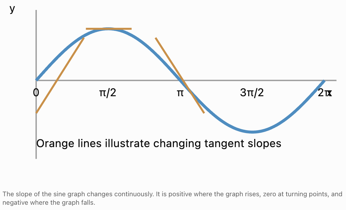
Differentiating the Sine Function
One of the fundamental results of calculus is:
d/dx (sin x) = cos x
This means that the instantaneous rate of change of sin x is cos x.
Why Is This True?
Using the definition of the derivative:
f′(x) = lim(h → 0) [sin(x + h) − sin x]/h
Apply the angle addition identity:
sin(x + h) = sin x cos h + cos x sin h
Substituting:
f′(x) = lim(h → 0) [sin x cos h + cos x sin h − sin x]/h
Group the terms:
= lim(h → 0) [sin x(cos h − 1)/h + cos x(sin h/h)]
We know:
lim(h → 0) (cos h − 1)/h = 0
and:
lim(h → 0) sin h/h = 1
Therefore:
f′(x) = sin x × 0 + cos x × 1
f′(x) = cos x
This derivation demonstrates why the fundamental trigonometric limits are so important.
Differentiating the Cosine Function
Another fundamental result is:
d/dx (cos x) = −sin x
This means that the instantaneous rate of change of cosine is negative sine.
Interpreting the Result
Consider:
y = cos x
At x = 0:
cos x is at a maximum.
Its slope is zero.
Since:
−sin 0 = 0
the derivative agrees with the graph.
At x = π/2:
cos x is decreasing most rapidly.
Since:
−sin(π/2) = −1
the slope is −1.
At x = π:
cos x is at a minimum.
Since:
−sin π = 0
the slope is zero again.
The derivative accurately describes the changing slope of the cosine graph.
Comparing Sine, Cosine, and Their Derivatives
|
Original function |
Derivative |
|---|---|
|
sin x |
cos x |
|
cos x |
−sin x |
|
−sin x |
−cos x |
|
−cos x |
sin x |
Notice that repeated differentiation produces a cycle.
Starting with sin x:
sin x → cos x → −sin x → −cos x → sin x
After four derivatives, the original function returns.
This is a remarkable property of trigonometric functions.
Visualizing the Derivative Relationship
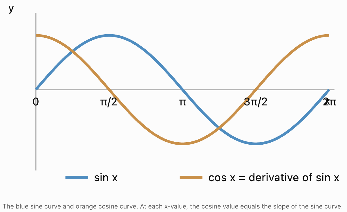
Worked Example: Finding the Slope of a Sine Graph
Consider:
y = sin x
Find the slope at:
x = π/3
Step 1: Differentiate
dy/dx = cos x
Step 2: Substitute
Slope = cos(π/3)
= 1/2
Slope = 0.5
Interpretation
At x = π/3, the sine graph is increasing with an instantaneous slope of 0.5.
Worked Example: Finding the Slope of a Cosine Graph
Consider:
y = cos x
Find the slope at:
x = π/6
Step 1: Differentiate
dy/dx = −sin x
Step 2: Substitute
Slope = −sin(π/6)
= −1/2
Slope = −0.5
Interpretation
At x = π/6, the cosine graph is decreasing with an instantaneous slope of −0.5.
Differentiating Trigonometric Functions with Coefficients
Trigonometric functions often contain constants that change their amplitude or frequency.
Consider:
y = A sin(kx)
Its derivative is:
dy/dx = Ak cos(kx)
Similarly:
y = A cos(kx)
has derivative:
dy/dx = −Ak sin(kx)
These results use the chain rule, an important differentiation technique.
Worked Example
Differentiate:
y = 4 sin(3x)
The amplitude coefficient is 4.
The coefficient inside the sine function is 3.
Therefore:
dy/dx = 4 × 3 cos(3x)
dy/dx = 12 cos(3x)
Another Example
Differentiate:
y = 5 cos(2x)
dy/dx = −5 × 2 sin(2x)
dy/dx = −10 sin(2x)
Understanding the Chain Rule
The chain rule is used to differentiate composite functions.
A composite function contains one function inside another.
For example:
y = sin(3x)
The outer function is sine.
The inner function is 3x.
The chain rule states:
dy/dx = (derivative of outer function) × (derivative of inner function)
For:
y = sin u
where u depends on x:
dy/dx = cos u × du/dx
Example
Differentiate:
y = sin(x²)
Let:
u = x²
Then:
du/dx = 2x
Therefore:
dy/dx = 2x cos(x²)
This illustrates how trigonometric differentiation extends beyond simple functions.
Differentiating Tangent
The tangent function can be written:
tan x = sin x/cos x
Using the quotient rule:
d/dx (tan x) = 1/cos²x
This is often written:
d/dx (tan x) = sec²x
where:
sec x = 1/cos x
The derivative exists wherever cos x is not zero.
Worked Example
Differentiate:
y = 3 tan x
Using the constant multiple rule:
dy/dx = 3 sec²x
This result is useful in advanced calculus, geometry, and engineering.
Rates of Change in Physical Systems
Trigonometric functions often model quantities that vary with time.
For example, the displacement of a vibrating object may be:
x(t) = A sin(ωt)
where:
-
x = displacement.
-
A = amplitude.
-
ω = angular frequency.
-
t = time.
The velocity is the derivative of displacement.
v(t) = dx/dt
Therefore:
v(t) = Aω cos(ωt)
Acceleration is the derivative of velocity.
a(t) = dv/dt
Therefore:
a(t) = −Aω² sin(ωt)
Since:
x(t) = A sin(ωt)
we obtain:
a(t) = −ω²x(t)
This relationship is fundamental to simple harmonic motion.


Worked Example: Displacement, Velocity, and Acceleration
A vibrating object moves according to:
x(t) = 0.05 sin(4πt)
where displacement is measured in metres and time in seconds.
Find expressions for velocity and acceleration.
Step 1: Identify the Constants
A = 0.05 m
ω = 4π rad/s
Step 2: Differentiate to Find Velocity
v(t) = 0.05 × 4π cos(4πt)
v(t) = 0.20π cos(4πt)
Step 3: Differentiate to Find Acceleration
a(t) = −0.20π × 4π sin(4πt)
a(t) = −0.80π² sin(4πt)
Step 4: Calculate Maximum Values
Maximum speed:
v_max = Aω
= 0.05 × 4π
v_max ≈ 0.628 m/s
Maximum acceleration magnitude:
a_max = Aω²
= 0.05 × (4π)²
a_max ≈ 7.90 m/s²
Interpretation
The object moves periodically, but its velocity and acceleration change continuously.
Calculus allows these quantities to be determined directly from the displacement function.
Circular Motion and Calculus
Consider a point moving around a circle of radius r at constant angular velocity ω.
Its coordinates are:
x(t) = r cos(ωt)
y(t) = r sin(ωt)
Differentiate to find the velocity components:
vₓ(t) = −rω sin(ωt)
vᵧ(t) = rω cos(ωt)
Differentiate again to find acceleration:
aₓ(t) = −rω² cos(ωt)
aᵧ(t) = −rω² sin(ωt)
The acceleration vector points toward the centre of the circle.
Its magnitude is:
a = rω²
This is the familiar centripetal acceleration formula.
Why This Matters
Trigonometry describes the position of a rotating object.
Calculus describes its velocity and acceleration.
Together, they provide a complete mathematical model of uniform circular motion.
Tangent Lines and Trigonometric Functions
A tangent line touches a smooth curve at a particular point and has the same instantaneous slope as the curve there.
For a function:
y = f(x)
the tangent line at x = a has slope:
m = f′(a)
The equation of the tangent line is:
y − f(a) = m(x − a)
Worked Example
Find the tangent line to:
y = sin x
at:
x = 0
Step 1: Find the Point
sin 0 = 0
The point is:
(0, 0)
Step 2: Find the Derivative
f′(x) = cos x
At x = 0:
m = cos 0
m = 1
Step 3: Write the Tangent Equation
y − 0 = 1(x − 0)
y = x
Interpretation
Near the origin, the sine curve is closely approximated by the straight line y = x.
This explains the small-angle approximation:
sin x ≈ x
for small angles in radians.
Increasing and Decreasing Trigonometric Functions
The derivative indicates whether a function is increasing or decreasing.
If:
f′(x) > 0
the function is increasing.
If:
f′(x) < 0
the function is decreasing.
If:
f′(x) = 0
the function has a stationary point, which may be a maximum, minimum, or another type of stationary point.
Example: Sine Function
For:
f(x) = sin x
the derivative is:
f′(x) = cos x
Between 0 and π/2:
cos x is positive.
Therefore, sin x is increasing.
Between π/2 and 3π/2:
cos x is negative.
Therefore, sin x is decreasing.
Between 3π/2 and 2π:
cos x is positive.
Therefore, sin x is increasing again.
This demonstrates how differentiation can be used to analyse trigonometric graphs.
Maximum and Minimum Values
Differentiation can help locate maximum and minimum values.
For a differentiable function, an interior local maximum or minimum must occur where the derivative is zero.
Consider:
f(x) = 3 sin x + 2
Differentiate:
f′(x) = 3 cos x
Set the derivative equal to zero:
3 cos x = 0
cos x = 0
Within the interval 0 ≤ x ≤ 2π:
x = π/2 or 3π/2
Evaluate the function.
At x = π/2:
f(π/2) = 3(1) + 2
f = 5
At x = 3π/2:
f(3π/2) = 3(−1) + 2
f = −1
Therefore:
Maximum value = 5
Minimum value = −1
These results also agree with the amplitude and vertical shift of the original function.
The Second Derivative
The second derivative describes the rate of change of the first derivative.
It is written:
f″(x)
For a position function, the first derivative gives velocity and the second derivative gives acceleration.
Example
Consider:
f(x) = sin x
First derivative:
f′(x) = cos x
Second derivative:
f″(x) = −sin x
Therefore:
f″(x) = −f(x)
This relationship is particularly important in wave motion and oscillations.
Physical Connection
Many oscillating systems satisfy equations of the form:
d²x/dt² = −ω²x
This means acceleration is proportional to displacement but acts in the opposite direction.
Sine and cosine functions naturally satisfy this relationship.
Introduction to Integration
Differentiation investigates rates of change.
Integration investigates accumulation.
An indefinite integral finds a family of functions whose derivative equals a given function.
For example:
Since:
d/dx (sin x) = cos x
we know:
∫ cos x dx = sin x + C
Similarly:
Since:
d/dx (cos x) = −sin x
we obtain:
∫ sin x dx = −cos x + C
Here, C is the constant of integration.
Why Is C Needed?
The derivative of a constant is zero.
Therefore, functions that differ only by a constant have the same derivative.
For example:
sin x
sin x + 3
sin x − 7
all have derivative cos x.
Definite Integrals and Area
A definite integral calculates signed accumulation over an interval.
It can represent the signed area between a graph and the x-axis.
Consider:
∫₀^π sin x dx
Using:
∫ sin x dx = −cos x + C
we evaluate:
[−cos x] from 0 to π
= −cos π − (−cos 0)
= 1 + 1
= 2
Therefore:
∫₀^π sin x dx = 2
Since sin x is nonnegative over this interval, the signed area is also the ordinary area between the curve and the x-axis.
Integration in Physics
Integration can be used to calculate displacement from velocity.
Suppose:
v(t) = 3 cos(2t)
Velocity is the derivative of displacement.
Therefore:
x(t) = ∫3 cos(2t) dt
Using the reverse chain rule:
x(t) = 1.5 sin(2t) + C
If the initial position is zero:
x(0) = 0
Then:
C = 0
Therefore:
x(t) = 1.5 sin(2t)
This illustrates how calculus can move between displacement and velocity models.
Trigonometric Functions in Advanced Mathematics
Trigonometric functions appear in many advanced mathematical topics.
Differential Equations
Differential equations describe relationships between functions and their derivatives.
They are used to model:
-
Oscillations.
-
Waves.
-
Electrical circuits.
-
Mechanical vibrations.
-
Population changes.
-
Dynamic systems.
Sine and cosine functions frequently appear as solutions to differential equations involving oscillation.
Fourier Analysis
Fourier analysis studies how complicated signals can be represented using combinations of sine and cosine functions.
It is used in:
-
Sound processing.
-
Image compression.
-
Medical imaging.
-
Communications.
-
Vibration analysis.
Complex Numbers
Euler's formula connects trigonometry with complex numbers:
e^(ix) = cos x + i sin x
where i² = −1.
This relationship is fundamental in advanced mathematics, electrical engineering, and signal processing.
Taylor Series
Taylor series allow functions to be approximated using polynomials.
For angles measured in radians:
sin x = x − x³/3! + x⁵/5! − ...
cos x = 1 − x²/2! + x⁴/4! − ...
These series explain why:
sin x ≈ x
and:
cos x ≈ 1 − x²/2
for small x.
Mathematical Modelling
Trigonometric calculus is used to model periodic phenomena in:
-
Physics.
-
Engineering.
-
Astronomy.
-
Economics.
-
Biology.
-
Computer science.


Choosing the Correct Calculus Method
|
Mathematical situation |
Useful method |
|---|---|
|
Function approaches a value |
Limits |
|
Trigonometric expression gives 0/0 |
Algebraic simplification and standard limits |
|
Slope between two points |
Average rate of change |
|
Slope at one point |
Derivative |
|
Rate of change of sin x |
cos x |
|
Rate of change of cos x |
−sin x |
|
Trigonometric function with an inner expression |
Chain rule |
|
Maximum or minimum value |
Derivative and critical points |
|
Velocity from displacement |
First derivative |
|
Acceleration from displacement |
Second derivative |
|
Displacement from velocity |
Integration |
|
Accumulation over an interval |
Definite integration |
|
Approximation near zero |
Small-angle approximation or Taylor series |
Common Mistakes
Using degrees instead of radians
Standard trigonometric derivative and limit formulas assume angles are measured in radians.
Assuming 0/0 is equal to zero
The expression 0/0 is indeterminate and requires further analysis.
Confusing a limit with direct substitution
A function may be undefined at a point even when its limit exists there.
Confusing average and instantaneous rates of change
Average rates use an interval, while instantaneous rates describe change at a particular point.
Forgetting the negative sign when differentiating cosine
The derivative of cos x is −sin x, not sin x.
Forgetting the chain rule
The derivative of sin(3x) is 3 cos(3x), not simply cos(3x).
Confusing a function with its derivative
The derivative describes the slope of the original function, not its height.
Assuming every stationary point is a maximum
A stationary point may be a maximum, minimum, or neither.
Ignoring the constant of integration
Indefinite integrals require a constant because many functions share the same derivative.
Confusing signed area with total geometric area
A definite integral can be negative when the graph lies below the x-axis.
Applying small-angle approximations to large angles
The approximations sin x ≈ x and tan x ≈ x are only accurate when x is sufficiently close to zero in radians.
Key Terms
-
Calculus: The branch of mathematics concerned with rates of change and accumulation.
-
Differential Calculus: The study of derivatives and instantaneous rates of change.
-
Integral Calculus: The study of accumulation and integration.
-
Limit: The value approached by a function as its input approaches a specified value.
-
Continuity: A property describing functions without a break at a particular point.
-
Indeterminate Form: An expression such as 0/0 that does not directly determine a limit.
-
Fundamental Trigonometric Limit: The result that sin x/x approaches 1 as x approaches zero in radians.
-
Squeeze Theorem: A method for determining a limit by bounding a function between two functions with the same limit.
-
Radian: An angular unit defined using arc length and radius.
-
Small-Angle Approximation: An approximation that simplifies trigonometric functions for angles near zero.
-
Average Rate of Change: The change in output divided by the change in input over an interval.
-
Instantaneous Rate of Change: The rate at which a function changes at a particular point.
-
Derivative: A function that describes instantaneous rates of change.
-
Differentiation: The process of finding a derivative.
-
Secant Line: A line passing through two points on a curve.
-
Tangent Line: A line whose slope matches the instantaneous slope of a curve at a point.
-
Chain Rule: A differentiation rule for composite functions.
-
Composite Function: A function formed by applying one function to the output of another.
-
First Derivative: The instantaneous rate of change of a function.
-
Second Derivative: The rate of change of the first derivative.
-
Stationary Point: A point where the derivative is zero.
-
Critical Point: A point where the derivative is zero or does not exist, provided the point is in the function's domain.
-
Local Maximum: A function value greater than or equal to nearby values.
-
Local Minimum: A function value less than or equal to nearby values.
-
Integration: The mathematical process of finding antiderivatives or accumulated quantities.
-
Indefinite Integral: A family of antiderivatives.
-
Definite Integral: A quantity representing signed accumulation over an interval.
-
Constant of Integration: An arbitrary constant added to an indefinite integral.
-
Differential Equation: An equation involving a function and one or more of its derivatives.
-
Fourier Analysis: The study of representing signals using combinations of sinusoidal functions.
-
Taylor Series: A polynomial series used to represent or approximate a function.
-
Euler's Formula: A relationship connecting exponential functions, complex numbers, and trigonometric functions.
-
Simple Harmonic Motion: Oscillation in which acceleration is proportional to displacement and directed toward equilibrium.
Key Takeaways
-
Trigonometry and calculus are closely connected because trigonometric functions describe continuously changing, periodic quantities.
-
Calculus investigates instantaneous rates of change and accumulation.
-
Limits provide the mathematical foundation for derivatives and integrals.
-
The fundamental trigonometric limit is lim(x → 0) sin x/x = 1 when x is measured in radians.
-
Another important limit is lim(x → 0) (1 − cos x)/x = 0.
-
The small-angle approximation sin x ≈ x is useful when x is close to zero in radians.
-
Average rate of change is calculated over an interval.
-
Instantaneous rate of change is represented by the derivative.
-
The derivative describes the slope of a curve at a particular point.
-
The derivative of sin x is cos x.
-
The derivative of cos x is −sin x.
-
Repeated differentiation of sine and cosine produces a repeating cycle.
-
The chain rule allows composite trigonometric functions to be differentiated.
-
Derivatives can identify where functions are increasing or decreasing.
-
Stationary points can be investigated to find maximum and minimum values.
-
The first derivative of displacement gives velocity.
-
The second derivative of displacement gives acceleration.
-
Circular motion can be analysed using trigonometric position functions and their derivatives.
-
Simple harmonic motion is closely connected to second-order differential equations.
-
Integration reverses differentiation and can calculate accumulated quantities.
-
Fourier analysis uses sine and cosine functions to represent complex signals.
-
Euler's formula connects trigonometric functions with complex numbers and exponential functions.
-
Taylor series provide polynomial approximations for trigonometric functions.
-
Trigonometric calculus is widely used in physics, engineering, signal processing, and advanced mathematics.
Check Your Understanding
Recall and Understanding
-
Explain the difference between differential calculus and integral calculus.
-
Define a limit and explain why limits are important in calculus.
-
State the fundamental trigonometric limit involving sin x/x.
-
Explain why radians are important when differentiating trigonometric functions.
-
Describe the relationship between a function's graph and its derivative.
Application
-
Evaluate lim(x → 0) sin(4x)/x.
-
Evaluate lim(x → 0) sin(2x)/sin(5x).
-
Differentiate y = 6 sin x.
-
Differentiate y = 4 cos(3x).
-
Find the slope of y = sin x at x = π/4.
Analysis and Challenge
-
Use the fundamental trigonometric limit to evaluate lim(x → 0) (1 − cos x)/x².
-
A vibrating object has displacement x(t) = 0.08 sin(5t). Find expressions for its velocity and acceleration, then calculate its maximum speed and acceleration magnitude.
-
A point moves around a circle according to x(t) = 3 cos(2t) and y(t) = 3 sin(2t). Find its velocity components and calculate its constant speed.
-
Find the stationary points of f(x) = 2 sin x + 1 over the interval 0 ≤ x ≤ 2π, and classify them as maxima or minima.
-
Explain how trigonometric functions, differentiation, integration, and differential equations work together to describe oscillating physical systems.
Final Summary
Trigonometry provides mathematical models for angles, circular motion, and periodic behaviour, while calculus explains how these quantities change and accumulate.
Limits establish the foundations of differentiation, including the important relationship that sin x/x approaches 1 as x approaches zero in radians.
Differentiation reveals that the rate of change of sine is cosine, while the rate of change of cosine is negative sine.
These relationships make trigonometric functions particularly useful for describing velocity, acceleration, circular motion, and oscillations.
Integration allows accumulated quantities to be calculated and provides a way to recover displacement from velocity.
More advanced topics, including differential equations, Fourier analysis, Taylor series, and complex numbers, build on these connections.
The central principle is that trigonometric functions describe repeating patterns, while calculus provides the tools needed to understand how those patterns change, how quickly they change, and how their effects accumulate over time.
5. Comprehensive Problem Solving
Learning outcomes
- I can solve complex multi-step trigonometric problems.
- I can integrate concepts from throughout the course.
- I can select efficient mathematical strategies.
- I can justify rigorous mathematical reasoning.
- I can communicate complete and accurate mathematical solutions.
Comprehensive Problem Solving
Introduction to Comprehensive Trigonometric Problem Solving
Trigonometry is much more than calculating unknown sides and angles in triangles. It is a powerful mathematical system used to investigate geometric relationships, model periodic behaviour, analyse motion, solve equations, and explain real-world phenomena.
In advanced trigonometric problems, several mathematical concepts often need to be combined.
A single problem might require students to:
-
Interpret a diagram and identify geometric relationships.
-
Apply the sine rule or cosine rule.
-
Use trigonometric identities to simplify expressions.
-
Solve equations involving multiple angles.
-
Analyse trigonometric graphs.
-
Model periodic motion using sine or cosine functions.
-
Resolve vectors into components.
-
Apply limits or derivatives.
-
Evaluate the accuracy and reasonableness of a mathematical solution.
The challenge is not simply remembering formulas. It is deciding which mathematical techniques to use, why they are appropriate, and how to combine them into a logical solution.
Effective problem solving requires mathematical knowledge, strategic thinking, careful calculations, and clear communication.


Understanding the Structure of Complex Problems
A complex trigonometric problem usually contains several connected stages.
For example, a navigation problem might involve:
-
Converting bearings into horizontal and vertical components.
-
Adding displacement vectors.
-
Calculating the magnitude of the resultant displacement.
-
Determining its direction.
-
Interpreting the result using the correct bearing convention.
A trigonometric modelling problem might involve:
-
Identifying the maximum and minimum values of a periodic quantity.
-
Calculating amplitude and midline.
-
Determining period and angular frequency.
-
Constructing a suitable sine or cosine function.
-
Solving the model for a particular value.
-
Interpreting all relevant solutions.
The key is to recognise that a complicated problem can often be divided into several simpler problems.
A Systematic Problem-Solving Framework
A reliable strategy is to use six stages.
Understand
Read the problem carefully.
Identify:
-
What information is given?
-
What must be calculated or proved?
-
Which quantities are unknown?
-
Are there diagrams, graphs, or tables?
-
What units are involved?
-
Are there restrictions on the answers?
Represent
Translate the information into mathematics.
Possible representations include:
-
A labelled triangle.
-
A coordinate diagram.
-
A trigonometric graph.
-
A vector diagram.
-
An equation.
-
A table of values.
-
A periodic function.
Plan
Select an appropriate method.
Ask:
-
Is the triangle right-angled?
-
Are two sides and an included angle known?
-
Is a trigonometric identity needed?
-
Is the problem periodic?
-
Would vector components simplify the situation?
-
Can symmetry reduce the number of calculations?
Solve
Carry out the calculations logically.
Show substitutions, transformations, and intermediate results.
Avoid rounding too early.
Verify
Check the solution.
Possible checks include:
-
Substituting answers into the original equation.
-
Comparing calculated values with the diagram.
-
Checking whether the angle is in the correct quadrant.
-
Confirming units.
-
Testing whether all solutions lie within the required interval.
Communicate
Present a clear final answer with:
-
Appropriate notation.
-
Relevant units.
-
Suitable precision.
-
Correct direction or interval.
-
A short interpretation when required.
Selecting an Efficient Mathematical Strategy
Different trigonometric situations require different methods.
|
Problem characteristic |
Useful strategy |
|---|---|
|
Right-angled triangle |
SOHCAHTOA or Pythagorean theorem |
|
Non-right triangle with an opposite side-angle pair |
Sine rule |
|
Two sides and included angle |
Cosine rule |
|
Three known sides |
Cosine rule |
|
Multiple forces or displacements |
Vector components |
|
Repeating behaviour |
Sine or cosine model |
|
Unknown amplitude or period |
Analyse maximum, minimum, and cycle length |
|
Trigonometric expression to simplify |
Identities and algebra |
|
Equation involving sin x or cos x |
Unit circle and reference angles |
|
Equation involving sin 2x or cos 2x |
Multiple-angle identities |
|
Equation involving sin²x or cos²x |
Pythagorean identities or substitution |
|
Angle or distance varying with time |
Trigonometric modelling and calculus |
|
Required proof |
Transform one side using established identities |
The most efficient method is usually the one that uses the available information directly and introduces the fewest unnecessary calculations.
Combining the Sine Rule and Cosine Rule
Some triangle problems require more than one trigonometric technique.
Worked Example: Surveying an Inaccessible Distance
Two observation points, A and B, are 120 m apart.
A distant object C is observed at:
-
Angle CAB = 48°.
-
Angle ABC = 67°.
Find the distances AC and BC.
Step 1: Find the Third Angle
Angles in a triangle sum to 180°.
C = 180° − 48° − 67°
C = 65°
Step 2: Apply the Sine Rule
BC/sin 48° = AC/sin 67° = 120/sin 65°
To calculate BC:
BC = 120 sin 48°/sin 65°
BC ≈ 98.4 m
To calculate AC:
AC = 120 sin 67°/sin 65°
AC ≈ 121.9 m
Step 3: Check the Results
The largest angle is 67°, so its opposite side AC should be the longest.
Our results satisfy this condition.
Final Answer
-
AC ≈ 121.9 m.
-
BC ≈ 98.4 m.
This example demonstrates how geometry and trigonometry can be used to measure distances that cannot be measured directly.

Solving Ambiguous Triangle Problems
The sine rule can produce more than one valid triangle when two sides and a non-included angle are known.
This is called the ambiguous case.
Worked Example
In triangle ABC:
-
A = 35°.
-
a = 8 cm.
-
b = 12 cm.
Find the possible values of angle B.
Using the sine rule:
a/sin A = b/sin B
Therefore:
sin B = b sin A/a
sin B = 12 sin 35°/8
sin B ≈ 0.86036
Step 1: Find the Principal Angle
B₁ = sin⁻¹(0.86036)
B₁ ≈ 59.35°
Step 2: Find the Second Possible Angle
Because sine is positive in Quadrants I and II:
B₂ = 180° − 59.35°
B₂ ≈ 120.65°
Step 3: Check Both Triangles
First possibility:
C₁ = 180° − 35° − 59.35°
C₁ ≈ 85.65°
Second possibility:
C₂ = 180° − 35° − 120.65°
C₂ ≈ 24.35°
Both values are positive.
Therefore, both triangles are valid.
Conclusion
Two possible triangles satisfy the given information.
This illustrates why inverse trigonometric functions must be interpreted carefully rather than accepted without checking geometric constraints.
Combining Geometry and Trigonometric Identities
Complex geometry problems sometimes involve expressions that can be simplified using identities.
Important identities include:
sin²θ + cos²θ = 1
tan θ = sin θ/cos θ
sin 2θ = 2sin θ cos θ
cos 2θ = cos²θ − sin²θ
cos 2θ = 1 − 2sin²θ
cos 2θ = 2cos²θ − 1
Worked Example: Simplifying a Geometric Expression
A geometric calculation produces:
E = (1 − cos 2θ)/sin θ
Simplify the expression.
Step 1: Identify an Identity
Use:
cos 2θ = 1 − 2sin²θ
Therefore:
1 − cos 2θ = 2sin²θ
Step 2: Substitute
E = 2sin²θ/sin θ
Step 3: Simplify
E = 2sin θ
This simplification is valid where sin θ ≠ 0, as required by the original denominator.
Why This Matters
The original expression appears complicated, but an identity reduces it to a simple function.
Recognising familiar mathematical structures is an important problem-solving skill.
Solving Multi-Step Trigonometric Equations
Advanced trigonometric equations may require identities, algebraic factorisation, and careful analysis of solution intervals.
Worked Example
Solve:
2sin²x − 3sin x + 1 = 0
for:
0° ≤ x < 360°
Step 1: Use Algebraic Substitution
Let:
u = sin x
The equation becomes:
2u² − 3u + 1 = 0
Step 2: Factorise
(2u − 1)(u − 1) = 0
Therefore:
u = 1/2
or:
u = 1
Step 3: Return to Trigonometry
sin x = 1/2
Solutions:
x = 30°, 150°
For:
sin x = 1
Solution:
x = 90°
Final Answer
x = 30°, 90°, 150°
Verification
Each solution satisfies the original equation.
For sin x = 1/2:
2(1/2)² − 3(1/2) + 1 = 0
For sin x = 1:
2(1)² − 3(1) + 1 = 0
Both are correct.
Equations Involving Multiple Angles
Worked Example
Solve:
sin 2x = cos x
for:
0° ≤ x < 360°
Step 1: Apply the Double-Angle Identity
sin 2x = 2sin x cos x
Therefore:
2sin x cos x = cos x
Step 2: Rearrange
2sin x cos x − cos x = 0
Factorise:
cos x(2sin x − 1) = 0
Step 3: Solve Each Factor
First:
cos x = 0
Solutions:
x = 90°, 270°
Second:
2sin x − 1 = 0
sin x = 1/2
Solutions:
x = 30°, 150°
Final Answer
x = 30°, 90°, 150°, 270°
Important Lesson
Do not divide both sides by cos x before considering whether cos x = 0.
Doing so would eliminate valid solutions.
Solving Trigonometric Equations in Radians
Calculus and advanced mathematics generally use radians.
Worked Example
Solve:
2cos²x − 1 = 0
for:
0 ≤ x < 2π
Step 1: Rearrange
2cos²x = 1
cos²x = 1/2
Step 2: Take Square Roots
cos x = ±1/√2
Step 3: Identify Solutions
Cosine has magnitude 1/√2 at reference angle π/4.
The four solutions are:
x = π/4, 3π/4, 5π/4, 7π/4
Verification
Substituting any solution gives:
2(1/2) − 1 = 0
All four values are valid.
Solving Trigonometric Inequalities
Inequalities require identifying intervals rather than isolated solutions.
Worked Example
Solve:
2sin x − 1 ≥ 0
for:
0° ≤ x ≤ 360°
Step 1: Rearrange
sin x ≥ 1/2
Step 2: Find Boundary Angles
sin x = 1/2
at:
x = 30°, 150°
Step 3: Determine the Interval
Sine is at least 1/2 between these angles.
Final Answer
30° ≤ x ≤ 150°
The endpoints are included because the inequality uses ≥.
Modelling Periodic Behaviour
Trigonometric functions are particularly useful for modelling repeating patterns.
A general sinusoidal model is:
y = A sin[B(x − C)] + D
where:
-
|A| = amplitude.
-
B determines the period.
-
C = horizontal shift.
-
D = vertical shift or midline.
For B ≠ 0, the period in radians is:
T = 2π/|B|
In degrees:
T = 360°/|B|
Worked Example: Modelling Water Level
The water level in a harbour changes periodically.
The maximum water level is 8 m.
The minimum water level is 2 m.
The time between successive high tides is 12 hours.
At t = 0, the water level is at its maximum.
Construct a suitable trigonometric model.
Step 1: Calculate Amplitude
A = (Maximum − Minimum)/2
A = (8 − 2)/2
A = 3 m
Step 2: Calculate Midline
D = (Maximum + Minimum)/2
D = (8 + 2)/2
D = 5 m
Step 3: Determine Angular Frequency
Period:
T = 12 hours
B = 2π/T
B = 2π/12
B = π/6 rad/hour
Step 4: Choose a Function
Because the water level begins at a maximum, cosine is convenient.
h(t) = 5 + 3cos(πt/6)
Step 5: Verify
At t = 0:
h(0) = 5 + 3(1)
h(0) = 8 m
At t = 6:
h(6) = 5 + 3cos π
= 5 − 3
h(6) = 2 m
At t = 12:
h(12) = 5 + 3cos 2π
h(12) = 8 m
The model correctly reproduces the maximum, minimum, and period.


Extending the Model: Finding Specific Times
Using:
h(t) = 5 + 3cos(πt/6)
Find when the water level is 6.5 m during the first 12 hours.
Step 1: Form an Equation
6.5 = 5 + 3cos(πt/6)
Step 2: Rearrange
1.5 = 3cos(πt/6)
cos(πt/6) = 0.5
Step 3: Find the Angles
For one complete cycle:
πt/6 = π/3
or:
πt/6 = 5π/3
Step 4: Solve for Time
First solution:
t = 2 hours
Second solution:
t = 10 hours
Final Answer
The water level is 6.5 m at t = 2 hours and t = 10 hours.
Interpretation
The water reaches this height once while falling and once while rising.
This is why periodic modelling problems often have multiple valid solutions.
Combining Trigonometric Modelling and Calculus
The same water-level model can be used to investigate rates of change.
Given:
h(t) = 5 + 3cos(πt/6)
Differentiate with respect to time:
h′(t) = −(π/2)sin(πt/6)
The derivative measures how quickly the water level is rising or falling.
Worked Example
Find the rate of change at t = 3 hours.
h′(3) = −(π/2)sin(π/2)
= −π/2
h′(3) ≈ −1.57 m/hour
Interpretation
After three hours, the water level is falling at approximately 1.57 m/hour.
The negative sign indicates decreasing water level.
Further Analysis
The maximum rate of rise is:
π/2 m/hour
The maximum rate of fall has the same magnitude.
This illustrates how trigonometric models and derivatives can be combined to analyse physical systems.
Comprehensive Vector Problems
Trigonometry is frequently combined with vector methods in navigation, engineering, and physics.
Worked Example: Aircraft Navigation
An aircraft flies at 240 km/h relative to the air on a bearing of 060°.
A wind blows due south at 40 km/h.
Calculate the aircraft's ground speed and bearing.
Step 1: Choose Coordinates
Take:
-
East as positive x.
-
North as positive y.
Step 2: Resolve Aircraft Velocity
For bearings measured clockwise from north:
vₓ = v sin β
vᵧ = v cos β
Therefore:
vₓ = 240 sin 60°
vₓ ≈ 207.85 km/h
vᵧ = 240 cos 60°
vᵧ = 120 km/h
Step 3: Resolve Wind Velocity
The wind blows south.
Therefore:
wₓ = 0
wᵧ = −40 km/h
Step 4: Calculate Ground Velocity Components
Rₓ = 207.85 + 0
Rₓ ≈ 207.85 km/h
Rᵧ = 120 − 40
Rᵧ = 80 km/h
Step 5: Calculate Ground Speed
R = √(207.85² + 80²)
R ≈ 222.71 km/h
Step 6: Calculate Bearing
The angle east of north is:
β = tan⁻¹(207.85/80)
β ≈ 68.95°
Final Answer
Ground speed ≈ 222.7 km/h
Bearing ≈ 069°
Interpretation
The southerly wind reduces the aircraft's northward velocity, causing its ground track to be closer to east than its heading.
Comprehensive Force Problems
Engineering problems often involve several forces acting in different directions.
Worked Example: Resultant Force
Three forces act on an object:
-
F₁ = 80 N at 30° above the positive x-axis.
-
F₂ = 60 N at 150° counterclockwise from the positive x-axis.
-
F₃ = 40 N directly downward.
Find the resultant force.
Step 1: Resolve F₁
F₁ₓ = 80 cos 30°
F₁ₓ ≈ 69.28 N
F₁ᵧ = 80 sin 30°
F₁ᵧ = 40 N
Step 2: Resolve F₂
F₂ₓ = 60 cos 150°
F₂ₓ ≈ −51.96 N
F₂ᵧ = 60 sin 150°
F₂ᵧ = 30 N
Step 3: Resolve F₃
F₃ₓ = 0
F₃ᵧ = −40 N
Step 4: Add Horizontal Components
Rₓ = 69.28 − 51.96
Rₓ ≈ 17.32 N
Step 5: Add Vertical Components
Rᵧ = 40 + 30 − 40
Rᵧ = 30 N
Step 6: Calculate Magnitude
R = √(17.32² + 30²)
R ≈ 34.64 N
Step 7: Calculate Direction
θ = tan⁻¹(30/17.32)
θ ≈ 60°
Final Answer
Resultant force ≈ 34.64 N at 60° above the positive x-axis.
Verification
The positive horizontal and vertical components place the resultant in Quadrant I.
The direction is therefore consistent with the calculated components.
Combining Trigonometry with Circular Motion
Circular motion connects geometry, periodic functions, vectors, and calculus.
A point moving around a circle of radius r with constant angular velocity ω has coordinates:
x(t) = r cos(ωt)
y(t) = r sin(ωt)
Its velocity components are:
vₓ(t) = −rω sin(ωt)
vᵧ(t) = rω cos(ωt)
Its speed is:
v = rω
Its centripetal acceleration magnitude is:
a = rω²
Worked Example
A point moves around a circle of radius 2 m, completing one revolution every 4 seconds.
Calculate:
-
Angular velocity.
-
Speed.
-
Centripetal acceleration.
-
Position after 1 second, assuming it begins at (2, 0) and rotates counterclockwise.
Step 1: Angular Velocity
ω = 2π/T
= 2π/4
ω = π/2 rad/s
Step 2: Speed
v = rω
= 2 × π/2
v = π ≈ 3.14 m/s
Step 3: Centripetal Acceleration
a = rω²
= 2 × (π/2)²
a = π²/2 ≈ 4.93 m/s²
Step 4: Position After 1 Second
x(1) = 2cos(π/2)
x(1) = 0 m
y(1) = 2sin(π/2)
y(1) = 2 m
Final Answer
After 1 second, the point is at:
(0, 2)
The point has completed one-quarter of a revolution.

Comprehensive Problems Involving Trigonometric Proofs
A mathematical proof requires a logical sequence of justified steps.
Unlike numerical problems, a proof must demonstrate that a relationship is always true wherever both sides are defined.
Worked Example
Prove:
(1 − cos 2x)/sin 2x = tan x
where both sides are defined.
Step 1: Begin with the Left-Hand Side
LHS = (1 − cos 2x)/sin 2x
Step 2: Apply Double-Angle Identities
1 − cos 2x = 2sin²x
sin 2x = 2sin x cos x
Therefore:
LHS = 2sin²x/(2sin x cos x)
Step 3: Simplify
LHS = sin x/cos x
Step 4: Apply the Tangent Identity
sin x/cos x = tan x
Therefore:
LHS = RHS
The identity is proved for values where the original expressions are defined.
Why This Proof Is Rigorous
Each step follows from an established identity or valid algebraic simplification.
The proof does not rely on testing a few numerical examples.
Recognising When an Equation Is Not an Identity
An identity is true for all values in its domain.
An equation is generally true only for particular values.
Consider:
sin x = cos x
This is not an identity.
It is true only for certain angles.
Divide by cos x where cos x ≠ 0:
tan x = 1
Therefore:
x = 45° + 180°n
where n is any integer.
The distinction between an identity and an equation is essential for rigorous mathematical reasoning.
Trigonometric Substitution in Algebra
Trigonometric identities can simplify algebraic expressions containing square roots.
For example, consider:
√(1 − x²)
If:
x = sin θ
then:
1 − x² = 1 − sin²θ
Using the Pythagorean identity:
1 − sin²θ = cos²θ
Therefore:
√(1 − x²) = |cos θ|
If θ is restricted to −π/2 ≤ θ ≤ π/2, then cos θ ≥ 0, so:
√(1 − x²) = cos θ
This technique is called trigonometric substitution.
It is particularly useful in advanced calculus.
Numerical Methods and Approximation
Not every trigonometric equation has a convenient exact solution.
Some equations require numerical methods.
Consider:
sin x = x/2
where x is measured in radians.
One solution is:
x = 0
There are also nonzero solutions.
To locate a positive nonzero solution, define:
f(x) = sin x − x/2
We can investigate values numerically.
|
x |
f(x), approximately |
|---|---|
|
1.5 |
0.2475 |
|
1.8 |
0.0738 |
|
1.9 |
−0.0037 |
|
2.0 |
−0.0907 |
Because f(x) changes sign between 1.8 and 1.9 and is continuous, a root lies in that interval.
Using numerical refinement gives:
x ≈ 1.8955 radians
The corresponding negative solution is approximately −1.8955 radians.
Why Numerical Methods Matter
Many scientific and engineering models cannot be solved using simple algebraic rearrangement.
Numerical methods provide accurate approximations when exact solutions are difficult or unavailable.
Error Analysis and Reasonableness
A complete mathematical solution should include checks for accuracy.
Rounding Errors
Rounding intermediate values too early can produce inaccurate final answers.
For example, using:
sin 37° ≈ 0.6
may be adequate for an estimate but not for a precise calculation.
A calculator gives:
sin 37° ≈ 0.601815
Retaining more digits during intermediate calculations improves accuracy.
Measurement Uncertainty
Real-world measurements are rarely exact.
If an angle is measured as:
35° ± 1°
then a calculated distance may vary depending on the actual angle.
Model Limitations
A trigonometric model may assume:
-
Constant angular speed.
-
Perfectly periodic behaviour.
-
Negligible friction.
-
Constant environmental conditions.
-
Accurate measurements.
-
Ideal geometry.
A mathematically correct calculation can still produce a poor real-world prediction if these assumptions are unrealistic.
Evaluating a Mathematical Solution
A strong solution should answer the following questions.
Is the mathematics correct?
Check formulas, substitutions, identities, and calculations.
Are all solutions included?
Trigonometric equations often have multiple solutions.
Are the units appropriate?
Angles, distances, velocities, and forces require suitable units.
Is the answer physically possible?
A negative distance or an impossible triangle angle may indicate an error.
Is the answer sufficiently accurate?
Use appropriate significant figures and rounding.
Are the assumptions reasonable?
Consider whether the mathematical model represents the actual situation.
Is the reasoning clearly communicated?
Another person should be able to follow the steps and understand why they are valid.
Communicating Complete Mathematical Solutions
A well-presented solution normally includes:
-
A clear statement of the known information.
-
Definitions of unknown variables.
-
A suitable diagram or mathematical model when useful.
-
The relevant formulas or identities.
-
Correct substitutions and transformations.
-
Intermediate calculations.
-
Verification of the result.
-
A clearly identified final answer.
-
Appropriate units and interpretation.
Example of Weak Communication
"The answer is 18.4."
This does not explain the method, units, or meaning.
Example of Strong Communication
"Using the Pythagorean theorem, the resultant displacement is R = √(12² + 14²) ≈ 18.44 km. Since both components are positive, the displacement is northeast. The direction is θ = tan⁻¹(14/12) ≈ 49.4° north of east. Therefore, the resultant displacement is approximately 18.4 km at 49.4° north of east."
The second response demonstrates both mathematical understanding and clear communication.
Common Mistakes
Starting calculations without identifying the problem structure
Complex problems become easier when the known information and required result are clearly identified.
Choosing an inefficient method
A component method may be simpler than repeatedly applying the sine rule or cosine rule.
Confusing degrees and radians
Always check the calculator mode and the units expected by the problem.
Using inverse trigonometric functions without considering multiple solutions
A calculator may display only one principal angle.
Dividing by an expression that may equal zero
This can remove valid solutions from trigonometric equations.
Ignoring restrictions on solution intervals
Only solutions within the specified domain should be included.
Confusing identities with equations
An identity must hold throughout its domain, while an equation may hold only at particular values.
Applying identities incorrectly
Trigonometric identities must be used exactly and under valid algebraic conditions.
Rounding too early
Premature rounding can introduce significant errors in multi-step problems.
Ignoring the direction of vectors
Vector answers require both magnitude and direction.
Forgetting phase shifts in periodic models
An incorrect horizontal shift can produce a model that has the right amplitude and period but the wrong timing.
Assuming all real-world phenomena are perfectly periodic
Mathematical models are approximations and may require adjustments.
Failing to verify solutions
Extraneous solutions can arise during algebraic transformations.
Providing answers without mathematical reasoning
A correct numerical answer alone may not demonstrate a complete understanding of the problem.
Key Terms
-
Comprehensive Problem Solving: The process of combining multiple mathematical techniques to solve complex problems.
-
Mathematical Strategy: A planned method for approaching and solving a problem.
-
Mathematical Model: A mathematical representation of a real-world situation.
-
Trigonometric Ratio: A relationship involving angles and side lengths.
-
Sine Rule: A relationship between triangle sides and their opposite angles.
-
Cosine Rule: A relationship used to calculate unknown sides or angles in non-right triangles.
-
Ambiguous Case: A situation in which given triangle information may produce more than one valid triangle.
-
Trigonometric Identity: An equality that holds for all values where both sides are defined.
-
Trigonometric Equation: An equation involving trigonometric functions that must be solved for particular values.
-
Trigonometric Inequality: An inequality involving trigonometric expressions.
-
Reference Angle: The acute angle used to identify related trigonometric values.
-
Principal Value: The standard value returned by an inverse trigonometric function.
-
General Solution: An expression representing all solutions of a periodic equation.
-
Domain Restriction: A limitation on the values that a variable may take.
-
Periodic Function: A function that repeats its values at regular intervals.
-
Amplitude: The maximum distance of a periodic function from its midline.
-
Period: The interval required for one complete cycle.
-
Angular Frequency: The rate at which an angular phase changes, commonly measured in radians per second.
-
Phase Shift: A horizontal translation of a periodic function.
-
Midline: The central horizontal level around which a sinusoidal function oscillates.
-
Vector: A quantity with magnitude and direction.
-
Resultant Vector: A single vector representing the combined effect of multiple vectors.
-
Vector Component: The part of a vector acting along a specified direction.
-
Bearing: A direction measured clockwise from north.
-
Equilibrium: A condition in which the resultant force is zero.
-
Derivative: The instantaneous rate of change of a function.
-
Integration: A mathematical process used to determine antiderivatives or accumulated quantities.
-
Trigonometric Substitution: A method that uses trigonometric identities to simplify algebraic expressions.
-
Numerical Method: A computational technique for approximating mathematical solutions.
-
Approximation: A value close to an exact result.
-
Verification: The process of checking whether a proposed solution satisfies the original conditions.
-
Extraneous Solution: A result introduced during manipulation that does not satisfy the original equation.
-
Mathematical Proof: A logical demonstration that a mathematical statement is true.
-
Rigorous Reasoning: Mathematical reasoning supported by valid definitions, rules, and deductions.
-
Measurement Uncertainty: The range of possible values associated with an imperfect measurement.
-
Model Limitation: A condition under which a mathematical model may not accurately describe reality.
-
Mathematical Communication: The clear presentation of mathematical ideas, calculations, explanations, and conclusions.
Key Takeaways
-
Complex trigonometric problems often require several mathematical techniques to be combined into one coherent solution.
-
Effective problem solving begins with understanding the question and identifying the known and unknown quantities.
-
Diagrams, graphs, tables, and equations help represent complicated situations.
-
The most efficient mathematical strategy depends on the structure of the problem.
-
The sine rule and cosine rule are useful for solving non-right triangles.
-
The ambiguous case of the sine rule may produce two valid triangles.
-
Trigonometric identities can simplify complicated expressions and equations.
-
Factoring and algebraic substitution are valuable techniques for solving trigonometric equations.
-
Multiple-angle identities help solve equations involving expressions such as sin 2x and cos 2x.
-
Trigonometric inequalities require intervals rather than isolated solutions.
-
Sine and cosine functions are useful for modelling periodic phenomena.
-
Amplitude, period, midline, and phase shift determine the structure of sinusoidal models.
-
Periodic equations may produce several solutions within a specified interval.
-
Vector components allow forces, velocities, and displacements to be combined efficiently.
-
Navigation problems require careful interpretation of directions and bearings.
-
Circular motion connects trigonometry, angular velocity, and calculus.
-
Derivatives describe rates of change in trigonometric models.
-
Trigonometric proofs require logical transformations supported by valid identities.
-
Numerical methods are useful when exact algebraic solutions are unavailable.
-
Rounding should normally be delayed until the final stages of a calculation.
-
Real-world mathematical models depend on assumptions that should be evaluated.
-
Verification is an essential part of rigorous mathematical reasoning.
-
Complete solutions should communicate both the mathematical process and the meaning of the final result.
-
The goal of comprehensive problem solving is not simply to obtain an answer, but to develop a solution that is efficient, mathematically justified, accurate, and clearly communicated.
Check Your Understanding
Recall and Understanding
-
Explain why complex trigonometric problems often require more than one mathematical technique.
-
Describe the six stages of a systematic mathematical problem-solving process.
-
Explain how to choose between the sine rule and cosine rule.
-
Describe the difference between a trigonometric identity and a trigonometric equation.
-
Explain why checking the domain and solution interval is important when solving trigonometric equations.
Application
-
In triangle ABC, AB = 15 cm, AC = 12 cm, and angle BAC = 70°. Calculate BC and then determine the remaining two angles.
-
Solve 2cos²x − 3cos x + 1 = 0 for 0° ≤ x < 360°.
-
A Ferris wheel has a radius of 18 m and its centre is 20 m above the ground. It completes one revolution every 40 seconds. Construct a suitable cosine model for the height of a passenger who begins at the highest point.
-
A boat travels 25 km on a bearing of 045°, followed by 18 km on a bearing of 120°. Calculate its resultant displacement and bearing.
-
Prove the identity (1 − cos 2x)/sin 2x = tan x, stating any necessary domain restrictions.
Analysis and Challenge
-
A periodic function has a maximum value of 14, a minimum value of 2, and a period of 8 seconds. It begins at its minimum. Construct a suitable trigonometric model and determine when the function first reaches a value of 11.
-
Three forces act on an object: 75 N at 35° above the positive x-axis, 50 N at 140° counterclockwise from the positive x-axis, and 45 N downward. Calculate the resultant magnitude and direction.
-
A particle moves according to x(t) = 4cos(3t) and y(t) = 4sin(3t), where distances are measured in metres. Calculate its position at t = π/6 seconds, its speed, and its centripetal acceleration magnitude.
-
Solve sin 2x = sin x for 0 ≤ x < 2π. Explain why dividing by sin x at the beginning could lead to an incomplete solution.
-
Design a mathematical model for a real-world periodic phenomenon, such as tides, daylight hours, temperature, or mechanical vibration. Explain your choice of function, identify its parameters, solve a relevant prediction problem, and evaluate at least two limitations of your model.
Final Summary
Comprehensive trigonometric problem solving requires the ability to connect geometric reasoning, algebraic manipulation, trigonometric identities, equations, functions, vectors, and calculus.
Rather than treating each topic as an isolated collection of formulas, advanced mathematical reasoning involves recognising how these ideas work together.
Triangle geometry provides methods for determining unknown distances and angles.
Trigonometric identities and algebra allow complicated expressions to be simplified and equations to be solved.
Periodic functions provide models for repeating physical phenomena, while calculus extends these models to describe rates of change.
Vector methods allow directional quantities to be combined and interpreted in navigation, mechanics, and engineering.
Numerical techniques provide approximations when exact solutions are difficult to obtain.
Throughout the process, rigorous reasoning, verification, and mathematical communication are essential.
A successful comprehensive solution does more than produce the correct numerical result. It explains why the chosen method works, demonstrates accurate mathematical reasoning, checks the validity of the answer, and communicates a meaningful conclusion.