Trigonometry in Advanced Mathematics

Introduction

Many phenomena in the natural world follow repeating patterns.

The temperature rises and falls throughout the year. Ocean tides move between high and low levels. A Ferris wheel carries passengers through repeated cycles of height. Electrical signals oscillate, sound waves vibrate, and the amount of daylight changes with the seasons.

Although these situations appear very different, they share an important mathematical feature: periodicity.

A periodic phenomenon repeats its behaviour after a regular interval of time or distance.

Trigonometric functions, particularly sine and cosine, provide powerful tools for describing these patterns. By adjusting their amplitude, period, phase shift, and vertical translation, we can construct mathematical models that approximate real-world cycles.

These models allow us to describe observations, make predictions, compare different situations, and evaluate how accurately mathematics represents reality.

In this lesson, we will explore how to model periodic phenomena, interpret model parameters in context, analyse seasonal and cyclical data, construct models from measurements, and evaluate their accuracy and limitations.

Understanding Periodic Phenomena

A periodic phenomenon is a process that repeats at regular intervals.

Examples include:

• The rotation of a Ferris wheel.

• The motion of a pendulum for small oscillations.

• Seasonal temperature changes.

• Alternating electrical current.

• Repeated vibrations of a musical instrument.

• Daylight duration throughout the year.

• Some components of ocean tidal motion.

• The movement of a point on a rotating wheel.

A periodic function satisfies:

f(t + T) = f(t)

where T is the period.

This means that after an interval T, the function returns to the same value and repeats its pattern.

Periodic Versus Non-Periodic Behaviour

Not every changing quantity is periodic.

A car accelerating steadily does not necessarily follow a repeating pattern.

Similarly, a population growing exponentially is not periodic unless additional repeating influences affect its growth.

A phenomenon is suitable for basic trigonometric modelling when its values fluctuate around a central level in an approximately regular cycle.

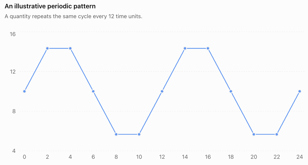
Notice that the pattern between time 0 and time 12 repeats between time 12 and time 24.

The period is 12 time units.

Learning Target 1: Modelling Periodic Phenomena Using Trigonometric Functions

The General Sinusoidal Model

The two most common functions used for periodic modelling are sine and cosine.

A general sine model is:

y = A sin[B(t − C)] + D

A general cosine model is:

y = A cos[B(t − C)] + D

where:

• A controls the amplitude and whether the graph is reflected.

• B controls the period.

• C represents the horizontal or phase shift.

• D represents the vertical shift or midline.

• t is the independent variable, often time.

• y is the quantity being modelled.

For these formulas, the angle inside sine or cosine is measured in radians.

Sine and Cosine as Periodic Models

The basic sine function:

y = sin t

starts at the midline and initially increases.

The basic cosine function:

y = cos t

starts at a maximum.

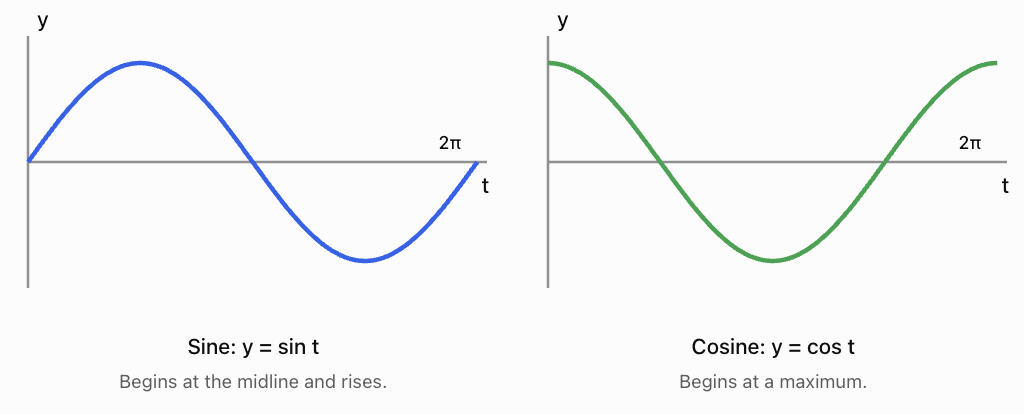
Both functions have:

• Amplitude = 1

• Period = 2π radians, or 360°

• Midline = 0

• Range from −1 to 1

They differ only in their horizontal positions.

Why Are Sine and Cosine Suitable?

Sine and cosine functions are useful because they are smooth, continuous, and periodic.

They can represent situations where a quantity:

1. Increases from a minimum toward a maximum.

2. Decreases from the maximum toward a minimum.

3. Repeats this pattern at regular intervals.

However, real-world data are rarely perfectly sinusoidal. A trigonometric function is often an approximation rather than an exact description.

Worked Example 1: Modelling a Ferris Wheel

A Ferris wheel has a radius of 15 m.

Its centre is 18 m above the ground.

The wheel completes one revolution every 40 seconds.

A passenger begins at the highest point.

Construct a function for the passenger's height.

Step 1: Identify the amplitude.

The passenger moves 15 m above and below the centre.

A = 15 m

Step 2: Identify the midline.

The wheel's centre is 18 m above the ground.

D = 18 m

Step 3: Determine the period.

T = 40 seconds

B = 2π/T

B = 2π/40 = π/20

Step 4: Choose the trigonometric function.

The passenger starts at the highest point.

Cosine is convenient because cos 0 = 1.

Therefore:

h(t) = 18 + 15 cos(πt/20)

where t is measured in seconds and h is measured in metres.

Step 5: Check important positions.

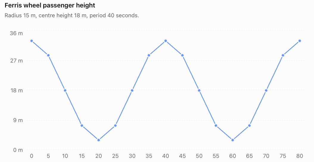
The model repeats every 40 seconds and predicts heights between 3 m and 33 m.

Learning Target 2: Interpreting Amplitude, Period, and Phase Shift in Context

Understanding the parameters of a trigonometric model is essential.

Each parameter describes a different feature of the periodic phenomenon.

Amplitude

For:

y = A sin[B(t − C)] + D

the amplitude is:

Amplitude = |A|

The amplitude measures the maximum distance from the midline.

If the maximum and minimum values are known:

Amplitude = (Maximum − Minimum)/2

For example, suppose a seasonal temperature varies between 12°C and 28°C.

Amplitude = (28 − 12)/2

Amplitude = 8°C

This means the temperature varies approximately 8°C above and below its average level.

Midline and Vertical Shift

The midline is the central value around which the function oscillates.

Midline = (Maximum + Minimum)/2

For the temperature example:

D = (28 + 12)/2

D = 20°C

The model oscillates around 20°C.

The predicted maximum is:

D + |A| = 28°C

The predicted minimum is:

D − |A| = 12°C

Period

The period is the time required for one complete cycle.

For a sine or cosine model:

T = 2π/|B|

Therefore:

|B| = 2π/T

If a phenomenon repeats every 12 months:

T = 12

B = 2π/12 = π/6

If a wheel rotates once every 30 seconds:

T = 30

B = 2π/30 = π/15

The units of B are radians per unit of time.

Phase Shift

The phase shift describes how far the basic sine or cosine graph is moved horizontally.

In:

y = A cos[B(t − C)] + D

the phase shift is C.

For positive A and B, the cosine function reaches a maximum at t = C.

For example:

y = 10 cos[(π/6)(t − 3)] + 20

has:

• Amplitude = 10

• Period = 12

• Phase shift = 3 units to the right

• Midline = 20

The first maximum occurs at t = 3, assuming t is measured from zero and the cycle is considered modulo its period.

Phase shifts can also be negative, representing movement to the left.

A Note About Equivalent Models

The same periodic function can often be represented in several ways.

For example:

sin t = cos(t − π/2)

Therefore, a sine model and a cosine model may describe exactly the same data.

Phase shifts are not unique because adding a whole period produces an equivalent model.

The interpretation of phase shift depends on the chosen form and sign convention.

Worked Example 2: Interpreting a Seasonal Model

A city's average monthly temperature is approximated by:

T(t) = 22 + 7 cos[(π/6)(t − 7)]

where t = 1 represents January, t = 2 represents February, and so on.

Interpret the model.

Amplitude

|A| = 7°C

The temperature varies approximately 7°C above and below its average.

Midline

D = 22°C

The average level of the model is 22°C.

Period

T = 2π/(π/6)

T = 12 months

The pattern repeats annually.

Phase shift

C = 7

The maximum occurs at t = 7, corresponding to July.

Maximum temperature

22 + 7 = 29°C

Minimum temperature

22 − 7 = 15°C

The model predicts a maximum of 29°C in July and a minimum of 15°C approximately six months later, in January.

Worked Example 3: Interpreting a Tidal Model

A simplified tidal height model is:

h(t) = 2.5 + 1.2 cos[(2π/12.4)t]

where h is measured in metres and t in hours.

Interpret the parameters.

• Amplitude = 1.2 m

• Midline = 2.5 m

• Period = 12.4 hours

• Phase shift = 0 hours

Maximum height:

2.5 + 1.2 = 3.7 m

Minimum height:

2.5 − 1.2 = 1.3 m

The model predicts a high tide every 12.4 hours.

This is a simplified representation. Actual tides contain several interacting periodic components and are influenced by local geography and weather.

Learning Target 3: Analysing Seasonal and Cyclical Data

Real-world measurements are not usually presented as equations. Instead, we often begin with a table of observations or a graph.

Our task is to identify whether the data show a repeating pattern and determine whether a trigonometric model would be appropriate.

Recognizing Patterns in Data

When examining cyclical data, look for:

• Repeated maximum and minimum values.

• Approximately equal intervals between successive peaks.

• A reasonably stable average level.

• Similar shapes across repeated cycles.

• Deviations from the pattern that might indicate measurement error or additional influences.

A useful first step is to plot the observations.

Worked Example 4: Analysing Seasonal Temperature Data

Suppose the following illustrative monthly average temperatures are recorded for a city.

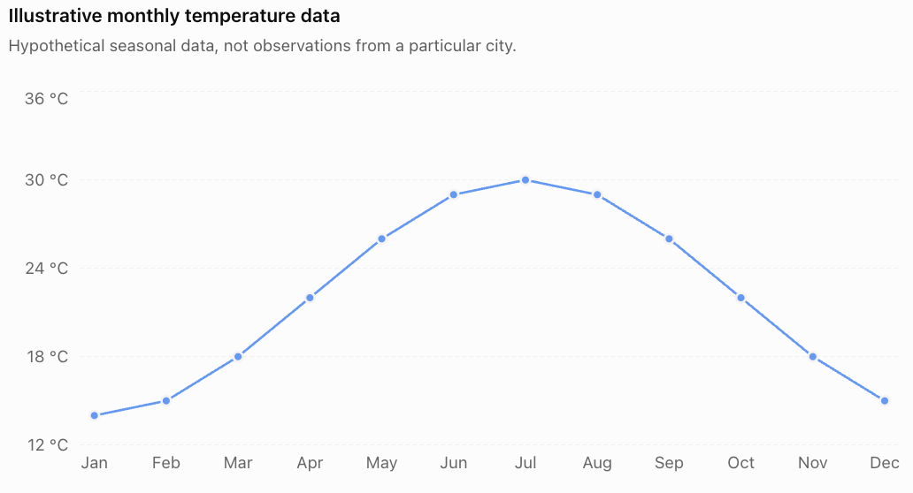
Step 1: Identify the maximum and minimum.

Maximum = 30°C

Minimum = 14°C

Step 2: Estimate the amplitude.

A = (30 − 14)/2

A = 8°C

Step 3: Estimate the midline.

D = (30 + 14)/2

D = 22°C

Step 4: Identify the period.

Seasonal temperature patterns generally repeat annually.

T = 12 months

B = 2π/12 = π/6

Step 5: Identify the phase shift.

The maximum occurs in July, month 7.

Using a cosine model:

T(t) = 22 + 8 cos[(π/6)(t − 7)]

Step 6: Interpret.

The model predicts a yearly cycle with a maximum of 30°C in July and a minimum of 14°C in January.

The observed temperatures are not perfectly sinusoidal, so the model is an approximation.

Comparing Observed and Predicted Values

The model fits these illustrative observations closely. That does not mean real seasonal temperature data will necessarily fit this well.

Analysing Daylight Hours

The duration of daylight changes throughout the year because Earth's axis is tilted relative to its orbit around the Sun.

At many mid-latitude locations, a sinusoidal model provides a useful first approximation to annual daylight variation.

Suppose a location experiences approximately:

• Maximum daylight = 15 hours

• Minimum daylight = 9 hours

• Maximum near day 172 of the year

Step 1: Find the amplitude.

A = (15 − 9)/2 = 3 hours

Step 2: Find the midline.

D = (15 + 9)/2 = 12 hours

Step 3: Find the period.

T ≈ 365 days

B = 2π/365

Step 4: Construct the model.

L(t) = 12 + 3 cos[(2π/365)(t − 172)]

where t is the day number of the year.

This model predicts approximately 15 hours of daylight near day 172 and 9 hours about half a year later.

Actual daylight duration depends on latitude and is not perfectly sinusoidal, especially near the polar regions.

Distinguishing Seasonal Cycles from Trends

A dataset may contain both a long-term trend and a repeating seasonal pattern.

For example, a temperature series might gradually increase over several decades while still fluctuating annually.

A model could take the form:

T(t) = mt + A sin[B(t − C)] + D

where mt represents a linear trend.

Such a model describes both the overall change and the periodic fluctuations.

However, it should only be used when the data support both features. A short dataset may not provide enough evidence to estimate a long-term trend reliably.

Learning Target 4: Creating Trigonometric Models from Real-World Data

Constructing a model involves determining suitable values for A, B, C, and D.

A systematic procedure makes this process much easier.

A Five-Step Modelling Procedure

Step 1: Determine the maximum and minimum.

Identify the highest and lowest values in the data.

Step 2: Calculate amplitude and midline.

Amplitude = (Maximum − Minimum)/2

Midline = (Maximum + Minimum)/2

Step 3: Determine the period.

Measure the time between consecutive peaks, consecutive troughs, or corresponding points in successive cycles.

Step 4: Calculate B.

B = 2π/T

Step 5: Determine the phase shift and choose sine or cosine.

Cosine is often convenient when the model begins at a maximum or minimum.

Sine is often convenient when the model begins at the midline.

These are choices of representation rather than strict requirements.

Worked Example 5: Constructing a Ferris Wheel Model from Data

A passenger's height on a Ferris wheel is recorded as follows:

Construct a trigonometric model.

Step 1: Determine maximum and minimum.

Maximum = 24 m

Minimum = 4 m

Step 2: Find amplitude.

A = (24 − 4)/2 = 10 m

Step 3: Find midline.

D = (24 + 4)/2 = 14 m

Step 4: Determine period.

The passenger reaches a minimum at t = 0 and again at t = 20.

T = 20 seconds

B = 2π/20 = π/10

Step 5: Choose a function.

The passenger starts at the minimum.

A negative cosine model is convenient:

h(t) = 14 − 10 cos(πt/10)

Step 6: Verify.

At t = 0:

h(0) = 14 − 10(1) = 4 m

At t = 10:

h(10) = 14 − 10 cos π

h(10) = 14 + 10 = 24 m

At t = 20:

h(20) = 14 − 10 cos 2π = 4 m

The model matches the observations.

Worked Example 6: Constructing a Sine Model

A rotating mechanism moves vertically between 2 cm and 14 cm.

It completes one cycle every 8 seconds.

At t = 0, the mechanism is at its midline and moving upward.

Construct a model.

Step 1: Amplitude.

A = (14 − 2)/2 = 6 cm

Step 2: Midline.

D = (14 + 2)/2 = 8 cm

Step 3: Period.

T = 8 seconds

B = 2π/8 = π/4

Step 4: Choose sine.

The mechanism begins at the midline and initially rises.

Therefore:

y(t) = 8 + 6 sin(πt/4)

Step 5: Verify important times.

At t = 0:

y = 8 cm

At t = 2:

y = 8 + 6 sin(π/2) = 14 cm

At t = 4:

y = 8 cm

At t = 6:

y = 8 + 6 sin(3π/2) = 2 cm

At t = 8:

y = 8 cm

The model describes one complete cycle.

Worked Example 7: Creating a Model from Maximum and Minimum Times

A periodic water-level model has:

• Maximum height = 5.2 m at t = 3 hours

• Minimum height = 1.6 m at t = 9 hours

• Approximately sinusoidal behaviour

Construct a model.

Step 1: Calculate amplitude.

A = (5.2 − 1.6)/2 = 1.8 m

Step 2: Calculate midline.

D = (5.2 + 1.6)/2 = 3.4 m

Step 3: Determine the period.

The time from maximum to minimum is half a period.

T/2 = 9 − 3 = 6 hours

T = 12 hours

Step 4: Calculate B.

B = 2π/12 = π/6

Step 5: Choose cosine.

The maximum occurs at t = 3.

h(t) = 3.4 + 1.8 cos[(π/6)(t − 3)]

Step 6: Verify.

At t = 3:

h(3) = 3.4 + 1.8 = 5.2 m

At t = 9:

h(9) = 3.4 + 1.8 cos π

h(9) = 3.4 − 1.8 = 1.6 m

The model satisfies the supplied conditions.

Modelling Data That Are Not Perfectly Sinusoidal

Real data often contain noise, irregularities, or several overlapping cycles.

For example, measured values might be:

These observations suggest a period of approximately 12 hours, a midline near 3.5 m, and an amplitude near 1.8 m.

An initial model could be:

h(t) = 3.5 + 1.8 sin(πt/6)

But this particular model begins at the midline and rises, whereas the observations reach a maximum around t = 3. That is consistent with the model's timing.

The model does not match every measurement exactly, and that is expected.

More advanced modelling uses sinusoidal regression to estimate parameters that minimize prediction errors across all observations.

Learning Target 5: Evaluating the Accuracy of Trigonometric Models

Creating a model is not the final step.

We must evaluate how well it represents the observed data and whether it is appropriate for making predictions.

A model can be mathematically correct but still describe the real phenomenon poorly.

Residuals

A residual is the difference between an observed value and the corresponding model prediction.

Residual = Observed value − Predicted value

A positive residual means the observation is higher than the prediction.

A negative residual means the observation is lower than the prediction.

Worked Example 8: Calculating Residuals

Suppose a model predicts the following temperatures:

The residuals are:

−1, +1, 0, −1, +1, 0

The errors are relatively small and alternate between positive and negative values.

There is no obvious consistent overprediction or underprediction in this small sample.

However, we would need a larger dataset to evaluate the model's overall reliability.

Mean Absolute Error

One way to measure accuracy is the mean absolute error (MAE).

MAE is the average of the absolute residuals.

MAE = Sum of absolute residuals / Number of observations

For the previous example:

MAE = (1 + 1 + 0 + 1 + 1 + 0)/6

MAE ≈ 0.67°C

This means the model's predictions differ from the observations by an average absolute amount of approximately 0.67°C.

A smaller MAE indicates a better fit when comparing models on the same dataset and scale.

Root Mean Square Error

Another common measure is the root mean square error (RMSE).

RMSE = √[(Sum of squared residuals)/n]

For the previous example:

RMSE = √[(1 + 1 + 0 + 1 + 1 + 0)/6]

RMSE = √(4/6)

RMSE ≈ 0.82°C

RMSE gives greater weight to large errors than MAE does.

This makes it useful when large prediction errors are particularly undesirable.

Interpreting Residual Patterns

Residuals should be examined, not merely summarized with one number.

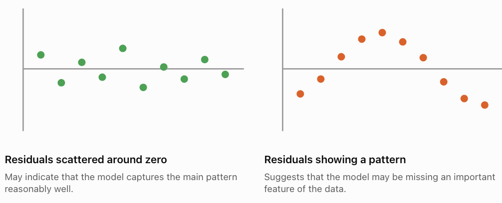
If residuals follow a repeating pattern, the model may have the wrong period, amplitude, or shape.

If residuals become progressively larger, the model may be missing a trend.

Worked Example 9: Comparing Two Models

Suppose two models are used to predict the same five observations.

Model A residuals:

−1, +1, 0, −1, +1

MAE(A) = (1 + 1 + 0 + 1 + 1)/5

MAE(A) = 0.8

Model B residuals:

−2, −2, +2, +2, −2

MAE(B) = (2 + 2 + 2 + 2 + 2)/5

MAE(B) = 2

Model A has the smaller MAE.

Conclusion: Model A fits these observations more closely according to mean absolute error.

However, a model should also be assessed on new data rather than only the observations used to construct it.

Interpolation and Extrapolation

Interpolation involves predicting values within the time range of the available data.

Extrapolation involves predicting values outside the observed time range.

For example, if temperature measurements are available for January through December, estimating a value for June is interpolation.

Predicting temperatures five years later is extrapolation.

Extrapolation is generally more uncertain because the periodic pattern may change over time.

Limitations of Trigonometric Models

A simple sinusoidal model assumes that:

• The period remains constant.

• The amplitude remains constant.

• The midline remains constant.

• The pattern is smooth and approximately symmetric.

• Random disturbances are relatively small.

These assumptions may not hold in reality.

For example, actual tides are influenced by multiple astronomical cycles, atmospheric pressure, wind, and coastal geography.

Seasonal temperatures are affected by weather variability and long-term climate changes.

A Ferris wheel model may be accurate during constant-speed rotation but less accurate while the wheel accelerates or stops.

Improving a Model

A model may be improved by:

• Collecting more observations.

• Measuring over several complete cycles.

• Using sinusoidal regression.

• Including additional periodic terms.

• Adding a trend when justified by the data.

• Examining residuals for systematic patterns.

• Testing predictions on observations not used to fit the model.

For a phenomenon containing two periodic components, a more advanced model might be:

y(t) = A₁ sin(B₁t + φ₁) + A₂ sin(B₂t + φ₂) + D

This type of model is useful for complex wave motion and tidal analysis.

Real-World Applications of Trigonometric Modelling

Engineering: Vibrations and Oscillations

Engineers use sinusoidal functions to approximate the motion of vibrating objects.

For example:

x(t) = 0.04 cos(10πt)

might describe a displacement of up to 0.04 m from equilibrium.

The amplitude is 0.04 m, and the period is:

T = 2π/(10π) = 0.2 s

The frequency is:

f = 1/T = 5 Hz

This means the object completes five oscillations each second.

The model assumes approximately simple harmonic motion with negligible damping.

Electricity: Alternating Current

Alternating voltage can be represented by:

V(t) = 170 sin(100πt)

where t is measured in seconds and V in volts.

The amplitude is 170 V.

The period is:

T = 2π/(100π) = 0.02 s

The frequency is:

f = 1/0.02 = 50 Hz

This model describes an ideal sinusoidal voltage signal.

Biology: Biological Rhythms

Many biological processes exhibit approximately periodic patterns.

Examples include sleep-wake cycles, daily hormone fluctuations, and body temperature rhythms.

A simplified body-temperature model might be:

T(t) = 37 + 0.3 cos[(π/12)(t − 17)]

where t is the hour of the day.

This model has:

• Midline = 37°C

• Amplitude = 0.3°C

• Period = 24 hours

• Maximum at 17:00, or 5 p.m.

This is an illustrative model, not a medical reference range or a universal description of human body temperature.

Environmental Science: Seasonal Daylight

Sinusoidal models can approximate annual changes in daylight duration.

These models can help explain patterns in solar-energy availability, plant growth, and seasonal environmental processes.

Astronomy: Repeating Motion

Trigonometric functions are used to describe periodic components of orbital motion, rotating objects, and observed wave signals.

For a perfectly circular orbit viewed from a suitable direction, a coordinate of the orbiting object may vary sinusoidally with time.

More complex orbits require additional mathematical relationships.

Common Mistakes

Mistake 1: Confusing Amplitude with Maximum Value

For:

y = 8 sin t + 20

the amplitude is 8, not 28.

The maximum is 28 and the minimum is 12.

Mistake 2: Confusing Period with B

For:

y = sin(4t)

the period is:

T = 2π/4 = π/2

It is not 4.

Mistake 3: Ignoring the Phase Shift

For:

y = 5 cos[2(t − 3)] + 10

the maximum occurs at t = 3, modulo the period, not necessarily at t = 0.

Mistake 4: Using Degrees Instead of Radians

In:

y = A sin[B(t − C)] + D

with B = 2π/T, the argument is measured in radians.

Use radian mode when evaluating the model on a calculator.

Mistake 5: Assuming All Cyclical Data Are Perfect Sine Waves

Real-world data may contain noise, asymmetry, trends, and several overlapping cycles.

A sinusoidal model is often an approximation.

Mistake 6: Choosing the Wrong Period

The time between a maximum and the next minimum is usually half a period for a simple sinusoid.

The full period is the time between corresponding points in successive cycles.

Mistake 7: Confusing Phase Shift with Vertical Shift

The phase shift moves the graph horizontally.

The vertical shift changes the midline.

Mistake 8: Ignoring Units

Amplitude has the same units as the dependent variable.

Period has units of time or another independent variable.

B has units of radians per unit of the independent variable.

Mistake 9: Rounding Too Early

Rounding amplitude, period, or phase shift too early may affect predictions.

Keep sufficient precision until the final result.

Mistake 10: Evaluating a Model Only at Its Peaks

A model may match the maximum and minimum but fit poorly at other times.

Always compare predictions with several observations throughout the cycle.

Key Terms

• Periodic phenomenon: A process that repeats at regular intervals.

• Periodic function: A function whose values repeat after a fixed interval.

• Sinusoidal function: A function represented by a transformed sine or cosine curve.

• Amplitude: The maximum distance between a periodic curve and its midline.

• Period: The interval required for one complete cycle.

• Frequency: The number of cycles completed per unit time.

• Phase shift: A horizontal translation of a periodic graph.

• Vertical shift: A movement of a graph upward or downward.

• Midline: The central level around which a sinusoidal function oscillates.

• Maximum: The greatest value attained by a function over a specified interval.

• Minimum: The smallest value attained by a function over a specified interval.

• Cycle: One complete repetition of a periodic pattern.

• Mathematical model: A mathematical representation of a real-world phenomenon.

• Seasonal variation: A repeating pattern associated with the seasons.

• Residual: The difference between an observed value and a predicted value.

• Mean absolute error: The average absolute difference between observed and predicted values.

• Root mean square error: A measure of prediction error that gives greater weight to larger errors.

• Interpolation: Estimating a value within the observed data range.

• Extrapolation: Predicting a value beyond the observed data range.

• Sinusoidal regression: A statistical technique for fitting sine or cosine models to data.

• Model validation: Testing how well a model represents observations, preferably including new data.

Key Takeaways

• Sine and cosine functions can model many approximately periodic phenomena.

• A general sinusoidal model is y = A sin[B(t − C)] + D or y = A cos[B(t − C)] + D.

• The amplitude is |A| and represents the maximum distance from the midline.

• The period is T = 2π/|B| when the argument is measured in radians.

• The phase shift describes the horizontal position of the cycle.

• The midline is D.

• Maximum and minimum values can be used to estimate amplitude and midline.

• The interval between successive peaks can be used to estimate the period.

• Real-world data can be modelled using estimated parameters or sinusoidal regression.

• Residuals and error measures help evaluate model accuracy.

• Models should be tested against observations and interpreted in context.

• A model that fits existing data well is not guaranteed to predict future behaviour accurately.

Check Your Understanding

The following questions address all five learning targets. Attempt them before reviewing the solutions.

Part A: Modelling Periodic Phenomena

Question 1

A Ferris wheel has a radius of 12 m and its centre is 15 m above the ground. It completes one revolution every 30 seconds. A passenger begins at the highest point.

Construct a model for the passenger's height.

Question 2

A vibrating object moves between −5 cm and +5 cm, completing one oscillation every 4 seconds. It begins at maximum displacement.

Write a cosine model for its displacement.

Part B: Interpreting Model Parameters

Question 3

Consider:

T(t) = 18 + 6 cos[(π/6)(t − 8)]

where t represents the month number.

Determine the amplitude, period, midline, phase shift, maximum, and minimum.

Question 4

A water-level model is:

h(t) = 3 + 1.5 sin[(π/4)t]

where t is measured in hours.

Determine the period and the first time after t = 0 when the maximum occurs.

Part C: Constructing Models from Data

Question 5

A periodic process has a maximum of 25, a minimum of 9, and a period of 10 seconds. It reaches a maximum at t = 2 seconds.

Construct a cosine model.

Question 6

A seasonal model has a maximum temperature of 32°C in July and a minimum of 20°C in January.

Assume a 12-month period.

Construct a cosine model using t = 1 for January.

Part D: Evaluating Models

Question 7

A model produces the following predictions:

Calculate the residuals and mean absolute error.

Question 8

Explain why a trigonometric model that fits one year of temperature data well may not predict temperatures accurately ten years into the future.

Part E: Integrated Problem Solving

Question 9

A Ferris wheel passenger's height is modelled by:

h(t) = 20 − 16 cos(πt/25)

where t is measured in seconds.

Calculate:

a) The maximum height.

b) The minimum height.

c) The period.

d) The height after 12.5 seconds.

e) The first time the passenger reaches the maximum height.

Question 10

A periodic water-level dataset has the following measurements:

Construct a sine model and explain how you would test its accuracy using additional measurements.

Check Your Understanding — Fully Worked Answers

Answer 1

Amplitude = radius = 12 m

Midline = centre height = 15 m

Period = 30 s

B = 2π/30 = π/15

The passenger starts at the maximum, so use cosine.

h(t) = 15 + 12 cos(πt/15)

Verification:

h(0) = 27 m

h(15) = 3 m

h(30) = 27 m

Answer 2

Amplitude = 5 cm

Midline = 0 cm

Period = 4 s

B = 2π/4 = π/2

The object begins at its maximum.

x(t) = 5 cos(πt/2)

Answer 3

Given:

T(t) = 18 + 6 cos[(π/6)(t − 8)]

Amplitude = 6°C

Period = 2π/(π/6) = 12 months

Midline = 18°C

Phase shift = 8 months to the right

Maximum = 18 + 6 = 24°C

Minimum = 18 − 6 = 12°C

The maximum occurs in August and the minimum approximately six months later, in February.

Answer 4

Given:

h(t) = 3 + 1.5 sin[(π/4)t]

Period:

T = 2π/(π/4)

T = 8 hours

The first maximum occurs when the sine argument equals π/2.

(π/4)t = π/2

t = 2 hours

Answer 5

Maximum = 25

Minimum = 9

Amplitude:

A = (25 − 9)/2 = 8

Midline:

D = (25 + 9)/2 = 17

Period = 10 s

B = 2π/10 = π/5

Maximum at t = 2.

y(t) = 17 + 8 cos[(π/5)(t − 2)]

Answer 6

Maximum = 32°C

Minimum = 20°C

Amplitude:

A = (32 − 20)/2 = 6°C

Midline:

D = (32 + 20)/2 = 26°C

Period = 12 months

B = π/6

Maximum occurs in July, t = 7.

T(t) = 26 + 6 cos[(π/6)(t − 7)]

Answer 7

Residual = Observed − Predicted

Residuals:

12 − 11 = +1

15 − 16 = −1

18 − 17 = +1

14 − 15 = −1

Mean absolute error:

MAE = (1 + 1 + 1 + 1)/4

MAE = 1

The model differs from the observations by an average absolute amount of one unit.

Answer 8

A model fitted to one year of data may not account for longer-term trends, unusual weather, changes in the seasonal pattern, or random variation.

The parameters may change over time, and the fitted model may capture features specific to the observed year.

To evaluate long-term predictive accuracy, we should test the model on additional years of observations and examine prediction errors.

Answer 9

Given:

h(t) = 20 − 16 cos(πt/25)

a) Maximum height

20 + 16 = 36 m

b) Minimum height

20 − 16 = 4 m

c) Period

T = 2π/(π/25)

T = 50 seconds

d) Height after 12.5 seconds

h(12.5) = 20 − 16 cos(π/2)

h(12.5) = 20 m

e) First maximum

The maximum occurs when cos(πt/25) = −1.

πt/25 = π

t = 25 seconds

Answer 10

Maximum = 5 m

Minimum = −1 m

Amplitude:

A = (5 − (−1))/2 = 3 m

Midline:

D = (5 + (−1))/2 = 2 m

The data return to the same midline position with the same direction of motion after 12 hours.

Period = 12 hours

B = 2π/12 = π/6

At t = 0, the water level is at the midline and increasing.

Therefore:

h(t) = 2 + 3 sin(πt/6)

Verification:

h(0) = 2 m

h(3) = 5 m

h(6) = 2 m

h(9) = −1 m

h(12) = 2 m

The model matches the five supplied observations.

To test its accuracy, collect additional measurements at intermediate times and during later cycles. Calculate residuals and MAE, then look for systematic errors.

Final Integrated Challenge: Modelling Seasonal Energy Production

A solar-energy facility records the following simplified monthly electricity production pattern:

• Maximum production: 900 MWh in June.

• Minimum production: 300 MWh in December.

• The cycle repeats approximately every 12 months.

Let t = 1 represent January.

Tasks

1. Determine the amplitude.

2. Determine the midline.

3. Determine the period and angular coefficient.

4. Construct a cosine model.

5. Predict electricity production in March and September.

6. Determine the months when production equals the midline.

7. Explain two limitations of the model.

Fully Worked Solution

Step 1: Calculate amplitude.

A = (900 − 300)/2

A = 300 MWh

Step 2: Calculate midline.

D = (900 + 300)/2

D = 600 MWh

Step 3: Determine the period.

T = 12 months

B = 2π/12 = π/6

Step 4: Construct the model.

The maximum occurs in June, month 6.

P(t) = 600 + 300 cos[(π/6)(t − 6)]

where P is measured in MWh.

Step 5: Predict March production.

March corresponds to t = 3.

P(3) = 600 + 300 cos[(π/6)(3 − 6)]

P(3) = 600 + 300 cos(−π/2)

P(3) = 600 MWh

Step 6: Predict September production.

September corresponds to t = 9.

P(9) = 600 + 300 cos[(π/6)(9 − 6)]

P(9) = 600 + 300 cos(π/2)

P(9) = 600 MWh

Step 7: Determine when production equals the midline.

Set:

600 + 300 cos[(π/6)(t − 6)] = 600

Therefore:

cos[(π/6)(t − 6)] = 0

Within one calendar year, the solutions are:

t = 3 and t = 9

Production equals the midline in March and September.

Step 8: Evaluate limitations.

The model assumes a constant annual period and a symmetric sinusoidal pattern.

Actual solar-energy production depends on weather, cloud cover, equipment performance, maintenance, daylight hours, and seasonal conditions.

The model also assumes that production reaches the same maximum and minimum every year, which may not occur.

Final Model Summary

The model provides a useful first approximation to seasonal production, but additional data are needed to assess its predictive accuracy.

Conclusion

Trigonometric modelling provides a powerful way to describe and analyse repeating patterns in the real world.

By using sine and cosine functions, we can represent periodic changes in height, temperature, daylight, electrical signals, vibrations, and other cyclical phenomena.

The amplitude, period, phase shift, and midline each describe an important feature of the pattern. Understanding these parameters allows us to interpret models and connect mathematical equations to physical situations.

We can construct models from observed data, use them to make predictions, and compare their predictions with actual measurements.

However, mathematical modelling also requires critical evaluation. Real-world cycles are rarely perfectly sinusoidal, and a model that fits existing observations may not always predict future behaviour accurately.

Successful trigonometric modelling combines mathematical techniques with data analysis, interpretation, verification, and an understanding of the limitations of real-world models.