Trigonometry in Advanced Mathematics
| Hệ thống: | Young Education |
| Khoá học: | Trigonometry |
| Book: | Trigonometry in Advanced Mathematics |
| Được in bởi: | Guest user |
| Ngày: | Thứ Hai, 9 tháng 11 2026, 4:36 PM |
1. Trigonometric Modelling
Learning outcomes
- I can model periodic phenomena using trigonometric functions.
- I can interpret amplitude, period, and phase shift in context.
- I can analyse seasonal and cyclical data.
- I can create trigonometric models from real-world data.
- I can evaluate the accuracy of models.
Introduction
Many phenomena in the natural world follow repeating patterns.
The temperature rises and falls throughout the year. Ocean tides move between high and low levels. A Ferris wheel carries passengers through repeated cycles of height. Electrical signals oscillate, sound waves vibrate, and the amount of daylight changes with the seasons.
Although these situations appear very different, they share an important mathematical feature: periodicity.
A periodic phenomenon repeats its behaviour after a regular interval of time or distance.
Trigonometric functions, particularly sine and cosine, provide powerful tools for describing these patterns. By adjusting their amplitude, period, phase shift, and vertical translation, we can construct mathematical models that approximate real-world cycles.
These models allow us to describe observations, make predictions, compare different situations, and evaluate how accurately mathematics represents reality.
In this lesson, we will explore how to model periodic phenomena, interpret model parameters in context, analyse seasonal and cyclical data, construct models from measurements, and evaluate their accuracy and limitations.
Understanding Periodic Phenomena
A periodic phenomenon is a process that repeats at regular intervals.
Examples include:
-
The rotation of a Ferris wheel.
-
The motion of a pendulum for small oscillations.
-
Seasonal temperature changes.
-
Alternating electrical current.
-
Repeated vibrations of a musical instrument.
-
Daylight duration throughout the year.
-
Some components of ocean tidal motion.
-
The movement of a point on a rotating wheel.
A periodic function satisfies:
f(t + T) = f(t)
where T is the period.
This means that after an interval T, the function returns to the same value and repeats its pattern.
Periodic Versus Non-Periodic Behaviour
Not every changing quantity is periodic.
A car accelerating steadily does not necessarily follow a repeating pattern.
Similarly, a population growing exponentially is not periodic unless additional repeating influences affect its growth.
A phenomenon is suitable for basic trigonometric modelling when its values fluctuate around a central level in an approximately regular cycle.
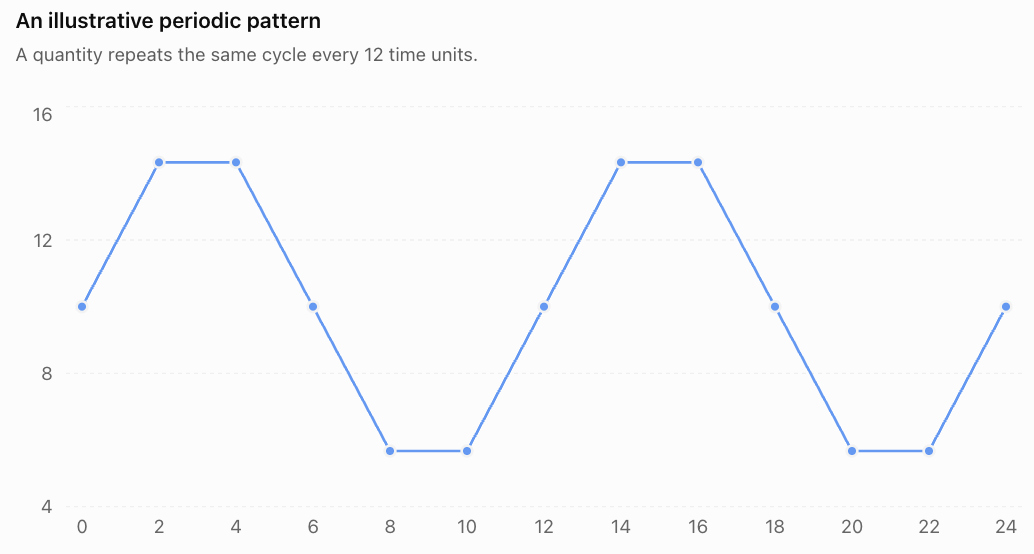
Notice that the pattern between time 0 and time 12 repeats between time 12 and time 24.
The period is 12 time units.
Learning Target 1: Modelling Periodic Phenomena Using Trigonometric Functions
The General Sinusoidal Model
The two most common functions used for periodic modelling are sine and cosine.
A general sine model is:
y = A sin[B(t − C)] + D
A general cosine model is:
y = A cos[B(t − C)] + D
where:
-
A controls the amplitude and whether the graph is reflected.
-
B controls the period.
-
C represents the horizontal or phase shift.
-
D represents the vertical shift or midline.
-
t is the independent variable, often time.
-
y is the quantity being modelled.
For these formulas, the angle inside sine or cosine is measured in radians.
Sine and Cosine as Periodic Models
The basic sine function:
y = sin t
starts at the midline and initially increases.
The basic cosine function:
y = cos t
starts at a maximum.
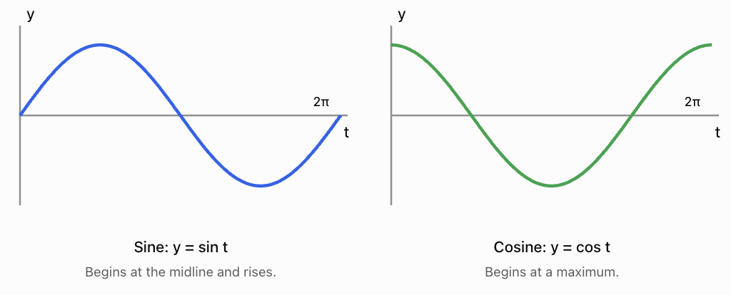
Both functions have:
-
Amplitude = 1
-
Period = 2π radians, or 360°
-
Midline = 0
-
Range from −1 to 1
They differ only in their horizontal positions.
Why Are Sine and Cosine Suitable?
Sine and cosine functions are useful because they are smooth, continuous, and periodic.
They can represent situations where a quantity:
-
Increases from a minimum toward a maximum.
-
Decreases from the maximum toward a minimum.
-
Repeats this pattern at regular intervals.
However, real-world data are rarely perfectly sinusoidal. A trigonometric function is often an approximation rather than an exact description.
Worked Example 1: Modelling a Ferris Wheel
A Ferris wheel has a radius of 15 m.
Its centre is 18 m above the ground.
The wheel completes one revolution every 40 seconds.
A passenger begins at the highest point.
Construct a function for the passenger's height.
Step 1: Identify the amplitude.
The passenger moves 15 m above and below the centre.
A = 15 m
Step 2: Identify the midline.
The wheel's centre is 18 m above the ground.
D = 18 m
Step 3: Determine the period.
T = 40 seconds
B = 2π/T
B = 2π/40 = π/20
Step 4: Choose the trigonometric function.
The passenger starts at the highest point.
Cosine is convenient because cos 0 = 1.
Therefore:
h(t) = 18 + 15 cos(πt/20)
where t is measured in seconds and h is measured in metres.
Step 5: Check important positions.
|
Time |
Position |
Height |
|---|---|---|
|
0 s |
Highest point |
33 m |
|
10 s |
Centre level |
18 m |
|
20 s |
Lowest point |
3 m |
|
30 s |
Centre level |
18 m |
|
40 s |
Highest point |
33 m |
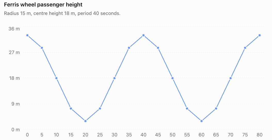
The model repeats every 40 seconds and predicts heights between 3 m and 33 m.
Learning Target 2: Interpreting Amplitude, Period, and Phase Shift in Context
Understanding the parameters of a trigonometric model is essential.
Each parameter describes a different feature of the periodic phenomenon.
Amplitude
For:
y = A sin[B(t − C)] + D
the amplitude is:
Amplitude = |A|
The amplitude measures the maximum distance from the midline.
If the maximum and minimum values are known:
Amplitude = (Maximum − Minimum)/2
For example, suppose a seasonal temperature varies between 12°C and 28°C.
Amplitude = (28 − 12)/2
Amplitude = 8°C
This means the temperature varies approximately 8°C above and below its average level.
Midline and Vertical Shift
The midline is the central value around which the function oscillates.
Midline = (Maximum + Minimum)/2
For the temperature example:
D = (28 + 12)/2
D = 20°C
The model oscillates around 20°C.
The predicted maximum is:
D + |A| = 28°C
The predicted minimum is:
D − |A| = 12°C
Period
The period is the time required for one complete cycle.
For a sine or cosine model:
T = 2π/|B|
Therefore:
|B| = 2π/T
If a phenomenon repeats every 12 months:
T = 12
B = 2π/12 = π/6
If a wheel rotates once every 30 seconds:
T = 30
B = 2π/30 = π/15
The units of B are radians per unit of time.
Phase Shift
The phase shift describes how far the basic sine or cosine graph is moved horizontally.
In:
y = A cos[B(t − C)] + D
the phase shift is C.
For positive A and B, the cosine function reaches a maximum at t = C.
For example:
y = 10 cos[(π/6)(t − 3)] + 20
has:
-
Amplitude = 10
-
Period = 12
-
Phase shift = 3 units to the right
-
Midline = 20
The first maximum occurs at t = 3, assuming t is measured from zero and the cycle is considered modulo its period.
Phase shifts can also be negative, representing movement to the left.
A Note About Equivalent Models
The same periodic function can often be represented in several ways.
For example:
sin t = cos(t − π/2)
Therefore, a sine model and a cosine model may describe exactly the same data.
Phase shifts are not unique because adding a whole period produces an equivalent model.
The interpretation of phase shift depends on the chosen form and sign convention.
Worked Example 2: Interpreting a Seasonal Model
A city's average monthly temperature is approximated by:
T(t) = 22 + 7 cos[(π/6)(t − 7)]
where t = 1 represents January, t = 2 represents February, and so on.
Interpret the model.
Amplitude
|A| = 7°C
The temperature varies approximately 7°C above and below its average.
Midline
D = 22°C
The average level of the model is 22°C.
Period
T = 2π/(π/6)
T = 12 months
The pattern repeats annually.
Phase shift
C = 7
The maximum occurs at t = 7, corresponding to July.
Maximum temperature
22 + 7 = 29°C
Minimum temperature
22 − 7 = 15°C
The model predicts a maximum of 29°C in July and a minimum of 15°C approximately six months later, in January.
Worked Example 3: Interpreting a Tidal Model
A simplified tidal height model is:
h(t) = 2.5 + 1.2 cos[(2π/12.4)t]
where h is measured in metres and t in hours.
Interpret the parameters.
-
Amplitude = 1.2 m
-
Midline = 2.5 m
-
Period = 12.4 hours
-
Phase shift = 0 hours
Maximum height:
2.5 + 1.2 = 3.7 m
Minimum height:
2.5 − 1.2 = 1.3 m
The model predicts a high tide every 12.4 hours.
This is a simplified representation. Actual tides contain several interacting periodic components and are influenced by local geography and weather.
Learning Target 3: Analysing Seasonal and Cyclical Data
Real-world measurements are not usually presented as equations. Instead, we often begin with a table of observations or a graph.
Our task is to identify whether the data show a repeating pattern and determine whether a trigonometric model would be appropriate.
Recognizing Patterns in Data
When examining cyclical data, look for:
-
Repeated maximum and minimum values.
-
Approximately equal intervals between successive peaks.
-
A reasonably stable average level.
-
Similar shapes across repeated cycles.
-
Deviations from the pattern that might indicate measurement error or additional influences.
A useful first step is to plot the observations.
Worked Example 4: Analysing Seasonal Temperature Data
Suppose the following illustrative monthly average temperatures are recorded for a city.
|
Month |
Temperature (°C) |
|---|---|
|
January |
14 |
|
February |
15 |
|
March |
18 |
|
April |
22 |
|
May |
26 |
|
June |
29 |
|
July |
30 |
|
August |
29 |
|
September |
26 |
|
October |
22 |
|
November |
18 |
|
December |
15 |
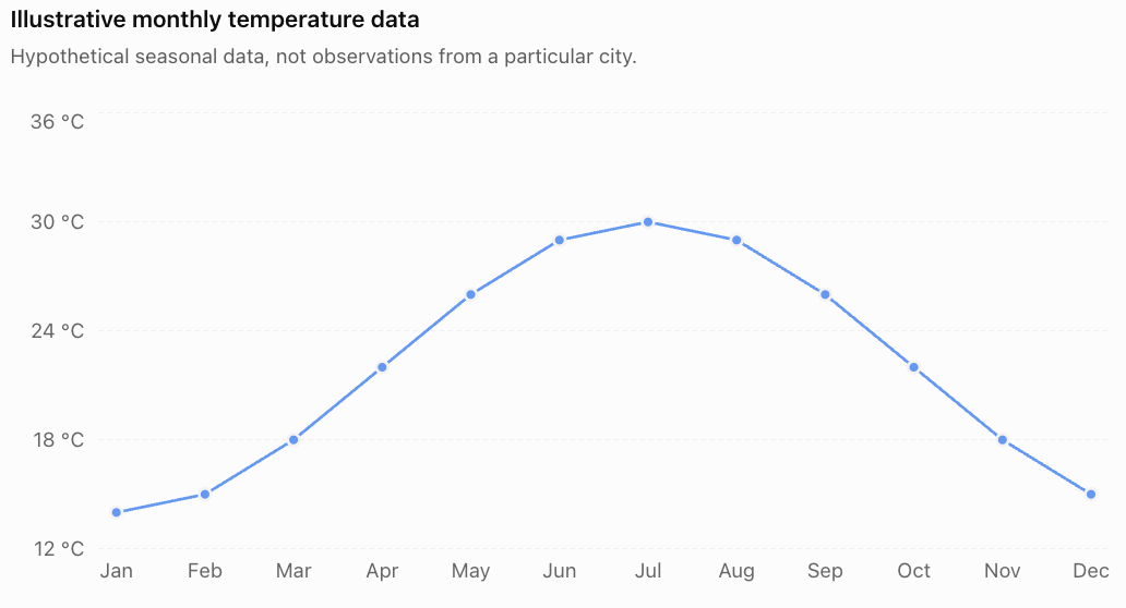
Step 1: Identify the maximum and minimum.
Maximum = 30°C
Minimum = 14°C
Step 2: Estimate the amplitude.
A = (30 − 14)/2
A = 8°C
Step 3: Estimate the midline.
D = (30 + 14)/2
D = 22°C
Step 4: Identify the period.
Seasonal temperature patterns generally repeat annually.
T = 12 months
B = 2π/12 = π/6
Step 5: Identify the phase shift.
The maximum occurs in July, month 7.
Using a cosine model:
T(t) = 22 + 8 cos[(π/6)(t − 7)]
Step 6: Interpret.
The model predicts a yearly cycle with a maximum of 30°C in July and a minimum of 14°C in January.
The observed temperatures are not perfectly sinusoidal, so the model is an approximation.
Comparing Observed and Predicted Values
|
Month |
Observed |
Predicted |
Error (Observed − Predicted) |
|---|---|---|---|
|
January |
14.00 |
14.00 |
0.00 |
|
February |
15.00 |
15.07 |
−0.07 |
|
March |
18.00 |
18.00 |
0.00 |
|
April |
22.00 |
22.00 |
0.00 |
|
May |
26.00 |
26.00 |
0.00 |
|
June |
29.00 |
28.93 |
+0.07 |
|
July |
30.00 |
30.00 |
0.00 |
|
August |
29.00 |
28.93 |
+0.07 |
|
September |
26.00 |
26.00 |
0.00 |
|
October |
22.00 |
22.00 |
0.00 |
|
November |
18.00 |
18.00 |
0.00 |
|
December |
15.00 |
15.07 |
−0.07 |
The model fits these illustrative observations closely. That does not mean real seasonal temperature data will necessarily fit this well.
Analysing Daylight Hours
The duration of daylight changes throughout the year because Earth's axis is tilted relative to its orbit around the Sun.
At many mid-latitude locations, a sinusoidal model provides a useful first approximation to annual daylight variation.
Suppose a location experiences approximately:
-
Maximum daylight = 15 hours
-
Minimum daylight = 9 hours
-
Maximum near day 172 of the year
Step 1: Find the amplitude.
A = (15 − 9)/2 = 3 hours
Step 2: Find the midline.
D = (15 + 9)/2 = 12 hours
Step 3: Find the period.
T ≈ 365 days
B = 2π/365
Step 4: Construct the model.
L(t) = 12 + 3 cos[(2π/365)(t − 172)]
where t is the day number of the year.
This model predicts approximately 15 hours of daylight near day 172 and 9 hours about half a year later.
Actual daylight duration depends on latitude and is not perfectly sinusoidal, especially near the polar regions.
Distinguishing Seasonal Cycles from Trends
A dataset may contain both a long-term trend and a repeating seasonal pattern.
For example, a temperature series might gradually increase over several decades while still fluctuating annually.
A model could take the form:
T(t) = mt + A sin[B(t − C)] + D
where mt represents a linear trend.
Such a model describes both the overall change and the periodic fluctuations.
However, it should only be used when the data support both features. A short dataset may not provide enough evidence to estimate a long-term trend reliably.
Learning Target 4: Creating Trigonometric Models from Real-World Data
Constructing a model involves determining suitable values for A, B, C, and D.
A systematic procedure makes this process much easier.
A Five-Step Modelling Procedure
Step 1: Determine the maximum and minimum.
Identify the highest and lowest values in the data.
Step 2: Calculate amplitude and midline.
Amplitude = (Maximum − Minimum)/2
Midline = (Maximum + Minimum)/2
Step 3: Determine the period.
Measure the time between consecutive peaks, consecutive troughs, or corresponding points in successive cycles.
Step 4: Calculate B.
B = 2π/T
Step 5: Determine the phase shift and choose sine or cosine.
Cosine is often convenient when the model begins at a maximum or minimum.
Sine is often convenient when the model begins at the midline.
These are choices of representation rather than strict requirements.
Worked Example 5: Constructing a Ferris Wheel Model from Data
A passenger's height on a Ferris wheel is recorded as follows:
|
Time (s) |
Height (m) |
|---|---|
|
0 |
4 |
|
5 |
14 |
|
10 |
24 |
|
15 |
14 |
|
20 |
4 |
|
25 |
14 |
|
30 |
24 |
|
35 |
14 |
|
40 |
4 |
Construct a trigonometric model.
Step 1: Determine maximum and minimum.
Maximum = 24 m
Minimum = 4 m
Step 2: Find amplitude.
A = (24 − 4)/2 = 10 m
Step 3: Find midline.
D = (24 + 4)/2 = 14 m
Step 4: Determine period.
The passenger reaches a minimum at t = 0 and again at t = 20.
T = 20 seconds
B = 2π/20 = π/10
Step 5: Choose a function.
The passenger starts at the minimum.
A negative cosine model is convenient:
h(t) = 14 − 10 cos(πt/10)
Step 6: Verify.
At t = 0:
h(0) = 14 − 10(1) = 4 m
At t = 10:
h(10) = 14 − 10 cos π
h(10) = 14 + 10 = 24 m
At t = 20:
h(20) = 14 − 10 cos 2π = 4 m
The model matches the observations.
Worked Example 6: Constructing a Sine Model
A rotating mechanism moves vertically between 2 cm and 14 cm.
It completes one cycle every 8 seconds.
At t = 0, the mechanism is at its midline and moving upward.
Construct a model.
Step 1: Amplitude.
A = (14 − 2)/2 = 6 cm
Step 2: Midline.
D = (14 + 2)/2 = 8 cm
Step 3: Period.
T = 8 seconds
B = 2π/8 = π/4
Step 4: Choose sine.
The mechanism begins at the midline and initially rises.
Therefore:
y(t) = 8 + 6 sin(πt/4)
Step 5: Verify important times.
At t = 0:
y = 8 cm
At t = 2:
y = 8 + 6 sin(π/2) = 14 cm
At t = 4:
y = 8 cm
At t = 6:
y = 8 + 6 sin(3π/2) = 2 cm
At t = 8:
y = 8 cm
The model describes one complete cycle.
Worked Example 7: Creating a Model from Maximum and Minimum Times
A periodic water-level model has:
-
Maximum height = 5.2 m at t = 3 hours
-
Minimum height = 1.6 m at t = 9 hours
-
Approximately sinusoidal behaviour
Construct a model.
Step 1: Calculate amplitude.
A = (5.2 − 1.6)/2 = 1.8 m
Step 2: Calculate midline.
D = (5.2 + 1.6)/2 = 3.4 m
Step 3: Determine the period.
The time from maximum to minimum is half a period.
T/2 = 9 − 3 = 6 hours
T = 12 hours
Step 4: Calculate B.
B = 2π/12 = π/6
Step 5: Choose cosine.
The maximum occurs at t = 3.
h(t) = 3.4 + 1.8 cos[(π/6)(t − 3)]
Step 6: Verify.
At t = 3:
h(3) = 3.4 + 1.8 = 5.2 m
At t = 9:
h(9) = 3.4 + 1.8 cos π
h(9) = 3.4 − 1.8 = 1.6 m
The model satisfies the supplied conditions.
Modelling Data That Are Not Perfectly Sinusoidal
Real data often contain noise, irregularities, or several overlapping cycles.
For example, measured values might be:
|
Time |
Observed height (m) |
|---|---|
|
0 |
3.5 |
|
3 |
5.1 |
|
6 |
3.3 |
|
9 |
1.8 |
|
12 |
3.4 |
|
15 |
5.3 |
|
18 |
3.5 |
|
21 |
1.7 |
|
24 |
3.3 |
These observations suggest a period of approximately 12 hours, a midline near 3.5 m, and an amplitude near 1.8 m.
An initial model could be:
h(t) = 3.5 + 1.8 sin(πt/6)
But this particular model begins at the midline and rises, whereas the observations reach a maximum around t = 3. That is consistent with the model's timing.
The model does not match every measurement exactly, and that is expected.
More advanced modelling uses sinusoidal regression to estimate parameters that minimize prediction errors across all observations.
Learning Target 5: Evaluating the Accuracy of Trigonometric Models
Creating a model is not the final step.
We must evaluate how well it represents the observed data and whether it is appropriate for making predictions.
A model can be mathematically correct but still describe the real phenomenon poorly.
Residuals
A residual is the difference between an observed value and the corresponding model prediction.
Residual = Observed value − Predicted value
A positive residual means the observation is higher than the prediction.
A negative residual means the observation is lower than the prediction.
Worked Example 8: Calculating Residuals
Suppose a model predicts the following temperatures:
|
Month |
Observed (°C) |
Predicted (°C) |
Residual (°C) |
|---|---|---|---|
|
January |
13 |
14 |
−1 |
|
February |
16 |
15 |
+1 |
|
March |
18 |
18 |
0 |
|
April |
21 |
22 |
−1 |
|
May |
27 |
26 |
+1 |
|
June |
29 |
29 |
0 |
The residuals are:
−1, +1, 0, −1, +1, 0
The errors are relatively small and alternate between positive and negative values.
There is no obvious consistent overprediction or underprediction in this small sample.
However, we would need a larger dataset to evaluate the model's overall reliability.
Mean Absolute Error
One way to measure accuracy is the mean absolute error (MAE).
MAE is the average of the absolute residuals.
MAE = Sum of absolute residuals / Number of observations
For the previous example:
MAE = (1 + 1 + 0 + 1 + 1 + 0)/6
MAE ≈ 0.67°C
This means the model's predictions differ from the observations by an average absolute amount of approximately 0.67°C.
A smaller MAE indicates a better fit when comparing models on the same dataset and scale.
Root Mean Square Error
Another common measure is the root mean square error (RMSE).
RMSE = √[(Sum of squared residuals)/n]
For the previous example:
RMSE = √[(1 + 1 + 0 + 1 + 1 + 0)/6]
RMSE = √(4/6)
RMSE ≈ 0.82°C
RMSE gives greater weight to large errors than MAE does.
This makes it useful when large prediction errors are particularly undesirable.
Interpreting Residual Patterns
Residuals should be examined, not merely summarized with one number.
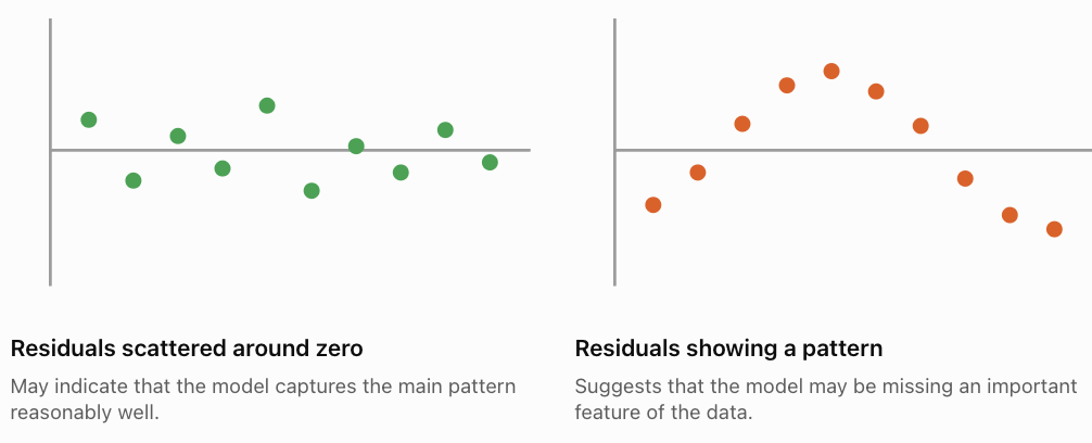
If residuals follow a repeating pattern, the model may have the wrong period, amplitude, or shape.
If residuals become progressively larger, the model may be missing a trend.
Worked Example 9: Comparing Two Models
Suppose two models are used to predict the same five observations.
|
Observation |
Actual |
Model A |
Model B |
|---|---|---|---|
|
1 |
10 |
11 |
12 |
|
2 |
14 |
13 |
16 |
|
3 |
18 |
18 |
16 |
|
4 |
14 |
15 |
12 |
|
5 |
10 |
9 |
12 |
Model A residuals:
−1, +1, 0, −1, +1
MAE(A) = (1 + 1 + 0 + 1 + 1)/5
MAE(A) = 0.8
Model B residuals:
−2, −2, +2, +2, −2
MAE(B) = (2 + 2 + 2 + 2 + 2)/5
MAE(B) = 2
Model A has the smaller MAE.
Conclusion: Model A fits these observations more closely according to mean absolute error.
However, a model should also be assessed on new data rather than only the observations used to construct it.
Interpolation and Extrapolation
Interpolation involves predicting values within the time range of the available data.
Extrapolation involves predicting values outside the observed time range.
For example, if temperature measurements are available for January through December, estimating a value for June is interpolation.
Predicting temperatures five years later is extrapolation.
Extrapolation is generally more uncertain because the periodic pattern may change over time.
Limitations of Trigonometric Models
A simple sinusoidal model assumes that:
-
The period remains constant.
-
The amplitude remains constant.
-
The midline remains constant.
-
The pattern is smooth and approximately symmetric.
-
Random disturbances are relatively small.
These assumptions may not hold in reality.
For example, actual tides are influenced by multiple astronomical cycles, atmospheric pressure, wind, and coastal geography.
Seasonal temperatures are affected by weather variability and long-term climate changes.
A Ferris wheel model may be accurate during constant-speed rotation but less accurate while the wheel accelerates or stops.
Improving a Model
A model may be improved by:
-
Collecting more observations.
-
Measuring over several complete cycles.
-
Using sinusoidal regression.
-
Including additional periodic terms.
-
Adding a trend when justified by the data.
-
Examining residuals for systematic patterns.
-
Testing predictions on observations not used to fit the model.
For a phenomenon containing two periodic components, a more advanced model might be:
y(t) = A₁ sin(B₁t + φ₁) + A₂ sin(B₂t + φ₂) + D
This type of model is useful for complex wave motion and tidal analysis.
Real-World Applications of Trigonometric Modelling
Engineering: Vibrations and Oscillations
Engineers use sinusoidal functions to approximate the motion of vibrating objects.
For example:
x(t) = 0.04 cos(10πt)
might describe a displacement of up to 0.04 m from equilibrium.
The amplitude is 0.04 m, and the period is:
T = 2π/(10π) = 0.2 s
The frequency is:
f = 1/T = 5 Hz
This means the object completes five oscillations each second.
The model assumes approximately simple harmonic motion with negligible damping.
Electricity: Alternating Current
Alternating voltage can be represented by:
V(t) = 170 sin(100πt)
where t is measured in seconds and V in volts.
The amplitude is 170 V.
The period is:
T = 2π/(100π) = 0.02 s
The frequency is:
f = 1/0.02 = 50 Hz
This model describes an ideal sinusoidal voltage signal.
Biology: Biological Rhythms
Many biological processes exhibit approximately periodic patterns.
Examples include sleep-wake cycles, daily hormone fluctuations, and body temperature rhythms.
A simplified body-temperature model might be:
T(t) = 37 + 0.3 cos[(π/12)(t − 17)]
where t is the hour of the day.
This model has:
-
Midline = 37°C
-
Amplitude = 0.3°C
-
Period = 24 hours
-
Maximum at 17:00, or 5 p.m.
This is an illustrative model, not a medical reference range or a universal description of human body temperature.
Environmental Science: Seasonal Daylight
Sinusoidal models can approximate annual changes in daylight duration.
These models can help explain patterns in solar-energy availability, plant growth, and seasonal environmental processes.
Astronomy: Repeating Motion
Trigonometric functions are used to describe periodic components of orbital motion, rotating objects, and observed wave signals.
For a perfectly circular orbit viewed from a suitable direction, a coordinate of the orbiting object may vary sinusoidally with time.
More complex orbits require additional mathematical relationships.
Common Mistakes
Mistake 1: Confusing Amplitude with Maximum Value
For:
y = 8 sin t + 20
the amplitude is 8, not 28.
The maximum is 28 and the minimum is 12.
Mistake 2: Confusing Period with B
For:
y = sin(4t)
the period is:
T = 2π/4 = π/2
It is not 4.
Mistake 3: Ignoring the Phase Shift
For:
y = 5 cos[2(t − 3)] + 10
the maximum occurs at t = 3, modulo the period, not necessarily at t = 0.
Mistake 4: Using Degrees Instead of Radians
In:
y = A sin[B(t − C)] + D
with B = 2π/T, the argument is measured in radians.
Use radian mode when evaluating the model on a calculator.
Mistake 5: Assuming All Cyclical Data Are Perfect Sine Waves
Real-world data may contain noise, asymmetry, trends, and several overlapping cycles.
A sinusoidal model is often an approximation.
Mistake 6: Choosing the Wrong Period
The time between a maximum and the next minimum is usually half a period for a simple sinusoid.
The full period is the time between corresponding points in successive cycles.
Mistake 7: Confusing Phase Shift with Vertical Shift
The phase shift moves the graph horizontally.
The vertical shift changes the midline.
Mistake 8: Ignoring Units
Amplitude has the same units as the dependent variable.
Period has units of time or another independent variable.
B has units of radians per unit of the independent variable.
Mistake 9: Rounding Too Early
Rounding amplitude, period, or phase shift too early may affect predictions.
Keep sufficient precision until the final result.
Mistake 10: Evaluating a Model Only at Its Peaks
A model may match the maximum and minimum but fit poorly at other times.
Always compare predictions with several observations throughout the cycle.
Key Terms
-
Periodic phenomenon: A process that repeats at regular intervals.
-
Periodic function: A function whose values repeat after a fixed interval.
-
Sinusoidal function: A function represented by a transformed sine or cosine curve.
-
Amplitude: The maximum distance between a periodic curve and its midline.
-
Period: The interval required for one complete cycle.
-
Frequency: The number of cycles completed per unit time.
-
Phase shift: A horizontal translation of a periodic graph.
-
Vertical shift: A movement of a graph upward or downward.
-
Midline: The central level around which a sinusoidal function oscillates.
-
Maximum: The greatest value attained by a function over a specified interval.
-
Minimum: The smallest value attained by a function over a specified interval.
-
Cycle: One complete repetition of a periodic pattern.
-
Mathematical model: A mathematical representation of a real-world phenomenon.
-
Seasonal variation: A repeating pattern associated with the seasons.
-
Residual: The difference between an observed value and a predicted value.
-
Mean absolute error: The average absolute difference between observed and predicted values.
-
Root mean square error: A measure of prediction error that gives greater weight to larger errors.
-
Interpolation: Estimating a value within the observed data range.
-
Extrapolation: Predicting a value beyond the observed data range.
-
Sinusoidal regression: A statistical technique for fitting sine or cosine models to data.
-
Model validation: Testing how well a model represents observations, preferably including new data.
Key Takeaways
-
Sine and cosine functions can model many approximately periodic phenomena.
-
A general sinusoidal model is y = A sin[B(t − C)] + D or y = A cos[B(t − C)] + D.
-
The amplitude is |A| and represents the maximum distance from the midline.
-
The period is T = 2π/|B| when the argument is measured in radians.
-
The phase shift describes the horizontal position of the cycle.
-
The midline is D.
-
Maximum and minimum values can be used to estimate amplitude and midline.
-
The interval between successive peaks can be used to estimate the period.
-
Real-world data can be modelled using estimated parameters or sinusoidal regression.
-
Residuals and error measures help evaluate model accuracy.
-
Models should be tested against observations and interpreted in context.
-
A model that fits existing data well is not guaranteed to predict future behaviour accurately.
Check Your Understanding
The following questions address all five learning targets. Attempt them before reviewing the solutions.
Part A: Modelling Periodic Phenomena
Question 1
A Ferris wheel has a radius of 12 m and its centre is 15 m above the ground. It completes one revolution every 30 seconds. A passenger begins at the highest point.
Construct a model for the passenger's height.
Question 2
A vibrating object moves between −5 cm and +5 cm, completing one oscillation every 4 seconds. It begins at maximum displacement.
Write a cosine model for its displacement.
Part B: Interpreting Model Parameters
Question 3
Consider:
T(t) = 18 + 6 cos[(π/6)(t − 8)]
where t represents the month number.
Determine the amplitude, period, midline, phase shift, maximum, and minimum.
Question 4
A water-level model is:
h(t) = 3 + 1.5 sin[(π/4)t]
where t is measured in hours.
Determine the period and the first time after t = 0 when the maximum occurs.
Part C: Constructing Models from Data
Question 5
A periodic process has a maximum of 25, a minimum of 9, and a period of 10 seconds. It reaches a maximum at t = 2 seconds.
Construct a cosine model.
Question 6
A seasonal model has a maximum temperature of 32°C in July and a minimum of 20°C in January.
Assume a 12-month period.
Construct a cosine model using t = 1 for January.
Part D: Evaluating Models
Question 7
A model produces the following predictions:
|
Observed |
Predicted |
|---|---|
|
12 |
11 |
|
15 |
16 |
|
18 |
17 |
|
14 |
15 |
Calculate the residuals and mean absolute error.
Question 8
Explain why a trigonometric model that fits one year of temperature data well may not predict temperatures accurately ten years into the future.
Part E: Integrated Problem Solving
Question 9
A Ferris wheel passenger's height is modelled by:
h(t) = 20 − 16 cos(πt/25)
where t is measured in seconds.
Calculate:
a) The maximum height.
b) The minimum height.
c) The period.
d) The height after 12.5 seconds.
e) The first time the passenger reaches the maximum height.
Question 10
A periodic water-level dataset has the following measurements:
|
Time |
Height (m) |
|---|---|
|
0 |
2 |
|
3 |
5 |
|
6 |
2 |
|
9 |
−1 |
|
12 |
2 |
Construct a sine model and explain how you would test its accuracy using additional measurements.
Check Your Understanding — Fully Worked Answers
Answer 1
Amplitude = radius = 12 m
Midline = centre height = 15 m
Period = 30 s
B = 2π/30 = π/15
The passenger starts at the maximum, so use cosine.
h(t) = 15 + 12 cos(πt/15)
Verification:
h(0) = 27 m
h(15) = 3 m
h(30) = 27 m
Answer 2
Amplitude = 5 cm
Midline = 0 cm
Period = 4 s
B = 2π/4 = π/2
The object begins at its maximum.
x(t) = 5 cos(πt/2)
Answer 3
Given:
T(t) = 18 + 6 cos[(π/6)(t − 8)]
Amplitude = 6°C
Period = 2π/(π/6) = 12 months
Midline = 18°C
Phase shift = 8 months to the right
Maximum = 18 + 6 = 24°C
Minimum = 18 − 6 = 12°C
The maximum occurs in August and the minimum approximately six months later, in February.
Answer 4
Given:
h(t) = 3 + 1.5 sin[(π/4)t]
Period:
T = 2π/(π/4)
T = 8 hours
The first maximum occurs when the sine argument equals π/2.
(π/4)t = π/2
t = 2 hours
Answer 5
Maximum = 25
Minimum = 9
Amplitude:
A = (25 − 9)/2 = 8
Midline:
D = (25 + 9)/2 = 17
Period = 10 s
B = 2π/10 = π/5
Maximum at t = 2.
y(t) = 17 + 8 cos[(π/5)(t − 2)]
Answer 6
Maximum = 32°C
Minimum = 20°C
Amplitude:
A = (32 − 20)/2 = 6°C
Midline:
D = (32 + 20)/2 = 26°C
Period = 12 months
B = π/6
Maximum occurs in July, t = 7.
T(t) = 26 + 6 cos[(π/6)(t − 7)]
Answer 7
Residual = Observed − Predicted
Residuals:
12 − 11 = +1
15 − 16 = −1
18 − 17 = +1
14 − 15 = −1
Mean absolute error:
MAE = (1 + 1 + 1 + 1)/4
MAE = 1
The model differs from the observations by an average absolute amount of one unit.
Answer 8
A model fitted to one year of data may not account for longer-term trends, unusual weather, changes in the seasonal pattern, or random variation.
The parameters may change over time, and the fitted model may capture features specific to the observed year.
To evaluate long-term predictive accuracy, we should test the model on additional years of observations and examine prediction errors.
Answer 9
Given:
h(t) = 20 − 16 cos(πt/25)
a) Maximum height
20 + 16 = 36 m
b) Minimum height
20 − 16 = 4 m
c) Period
T = 2π/(π/25)
T = 50 seconds
d) Height after 12.5 seconds
h(12.5) = 20 − 16 cos(π/2)
h(12.5) = 20 m
e) First maximum
The maximum occurs when cos(πt/25) = −1.
πt/25 = π
t = 25 seconds
Answer 10
Maximum = 5 m
Minimum = −1 m
Amplitude:
A = (5 − (−1))/2 = 3 m
Midline:
D = (5 + (−1))/2 = 2 m
The data return to the same midline position with the same direction of motion after 12 hours.
Period = 12 hours
B = 2π/12 = π/6
At t = 0, the water level is at the midline and increasing.
Therefore:
h(t) = 2 + 3 sin(πt/6)
Verification:
h(0) = 2 m
h(3) = 5 m
h(6) = 2 m
h(9) = −1 m
h(12) = 2 m
The model matches the five supplied observations.
To test its accuracy, collect additional measurements at intermediate times and during later cycles. Calculate residuals and MAE, then look for systematic errors.
Final Integrated Challenge: Modelling Seasonal Energy Production
A solar-energy facility records the following simplified monthly electricity production pattern:
-
Maximum production: 900 MWh in June.
-
Minimum production: 300 MWh in December.
-
The cycle repeats approximately every 12 months.
Let t = 1 represent January.
Tasks
-
Determine the amplitude.
-
Determine the midline.
-
Determine the period and angular coefficient.
-
Construct a cosine model.
-
Predict electricity production in March and September.
-
Determine the months when production equals the midline.
-
Explain two limitations of the model.
Fully Worked Solution
Step 1: Calculate amplitude.
A = (900 − 300)/2
A = 300 MWh
Step 2: Calculate midline.
D = (900 + 300)/2
D = 600 MWh
Step 3: Determine the period.
T = 12 months
B = 2π/12 = π/6
Step 4: Construct the model.
The maximum occurs in June, month 6.
P(t) = 600 + 300 cos[(π/6)(t − 6)]
where P is measured in MWh.
Step 5: Predict March production.
March corresponds to t = 3.
P(3) = 600 + 300 cos[(π/6)(3 − 6)]
P(3) = 600 + 300 cos(−π/2)
P(3) = 600 MWh
Step 6: Predict September production.
September corresponds to t = 9.
P(9) = 600 + 300 cos[(π/6)(9 − 6)]
P(9) = 600 + 300 cos(π/2)
P(9) = 600 MWh
Step 7: Determine when production equals the midline.
Set:
600 + 300 cos[(π/6)(t − 6)] = 600
Therefore:
cos[(π/6)(t − 6)] = 0
Within one calendar year, the solutions are:
t = 3 and t = 9
Production equals the midline in March and September.
Step 8: Evaluate limitations.
The model assumes a constant annual period and a symmetric sinusoidal pattern.
Actual solar-energy production depends on weather, cloud cover, equipment performance, maintenance, daylight hours, and seasonal conditions.
The model also assumes that production reaches the same maximum and minimum every year, which may not occur.
Final Model Summary
|
Parameter |
Value |
|---|---|
|
Amplitude |
300 MWh |
|
Midline |
600 MWh |
|
Period |
12 months |
|
Maximum |
900 MWh |
|
Minimum |
300 MWh |
|
Maximum month |
June |
|
Minimum month |
December |
|
March prediction |
600 MWh |
|
September prediction |
600 MWh |
The model provides a useful first approximation to seasonal production, but additional data are needed to assess its predictive accuracy.
Conclusion
Trigonometric modelling provides a powerful way to describe and analyse repeating patterns in the real world.
By using sine and cosine functions, we can represent periodic changes in height, temperature, daylight, electrical signals, vibrations, and other cyclical phenomena.
The amplitude, period, phase shift, and midline each describe an important feature of the pattern. Understanding these parameters allows us to interpret models and connect mathematical equations to physical situations.
We can construct models from observed data, use them to make predictions, and compare their predictions with actual measurements.
However, mathematical modelling also requires critical evaluation. Real-world cycles are rarely perfectly sinusoidal, and a model that fits existing observations may not always predict future behaviour accurately.
Successful trigonometric modelling combines mathematical techniques with data analysis, interpretation, verification, and an understanding of the limitations of real-world models.
2. Polar Coordinates and Parametric Curves
Learning outcomes
- I can define polar coordinates.
- I can convert between Cartesian and polar coordinates.
- I can graph simple polar equations.
- I can interpret parametric equations.
- I can connect multiple coordinate systems.
Introduction
Most of the mathematics we study begins with the Cartesian coordinate system. A point is described by two numbers, x and y, representing its horizontal and vertical positions.
However, Cartesian coordinates are not always the most convenient way to describe a location or a curve.
Imagine a radar operator tracking an aircraft. Rather than reporting how far east and north the aircraft is, it may be easier to describe its distance from the radar station and the direction in which it lies.
Similarly, a rotating wheel is easier to describe using a distance from its centre and an angle of rotation.
These situations lead to polar coordinates, which describe positions using a distance and an angle.
Another useful approach is to describe the coordinates of a moving point using a third variable, usually time. This leads to parametric equations.
Polar and parametric representations allow us to describe circles, spirals, curved paths, rotating objects, and complex geometric relationships in ways that are sometimes much simpler than ordinary Cartesian equations.
Understanding how these systems connect is an important foundation for advanced trigonometry, calculus, physics, engineering, and computer graphics.
Learning Target 1: Defining Polar Coordinates
What Are Polar Coordinates?
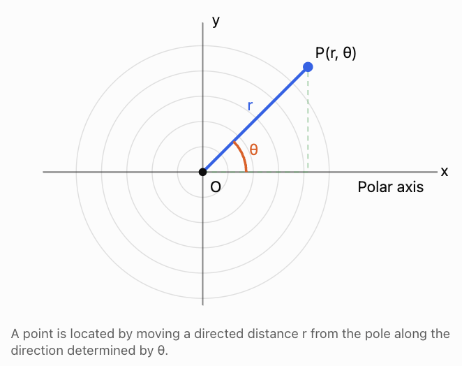
The polar coordinate system identifies a point using two values:
(r, θ)
where:
-
r is the directed distance from the origin.
-
θ is the angle measured from a fixed reference direction, normally the positive x-axis.
The origin is called the pole.
The positive x-axis is called the polar axis.
Angles are normally measured anticlockwise from the polar axis, although clockwise angles can be represented using negative values.
Understanding the Radius
For positive r, the point lies in the direction of angle θ.
For negative r, the point lies in the opposite direction.
For example:
(4, 30°)
means moving 4 units from the origin in the direction 30° anticlockwise from the positive x-axis.
But:
(−4, 30°)
means moving 4 units in the opposite direction, equivalent to a positive radius at 210°.
Understanding the Angle
Angles may be measured in degrees or radians.
Important equivalents include:
|
Degrees |
Radians |
|---|---|
|
0° |
0 |
|
30° |
π/6 |
|
45° |
π/4 |
|
60° |
π/3 |
|
90° |
π/2 |
|
180° |
π |
|
270° |
3π/2 |
|
360° |
2π |
In advanced mathematics, radians are normally preferred because they simplify calculus and many trigonometric formulas.
Worked Example 1: Plotting a Polar Point
Plot:
P = (5, 60°)
Step 1: Begin at the pole.
Step 2: Measure 60° anticlockwise from the positive x-axis.
Step 3: Move 5 units along that direction.
The resulting point lies in the first quadrant.
Worked Example 2: A Negative Radius
Interpret:
Q = (−3, 45°)
A negative radius means that the point lies in the direction opposite 45°.
The equivalent positive-radius angle is:
45° + 180° = 225°
Therefore:
(−3, 45°) = (3, 225°)
Both coordinate pairs represent the same point.
Why Polar Coordinates Are Not Unique
Unlike Cartesian coordinates, polar coordinates do not have a unique representation.
For example, the same point can be written as:
(4, 30°)
(4, 390°)
(4, −330°)
(−4, 210°)
Adding or subtracting a complete revolution does not change the location.
In general:
(r, θ) = (r, θ + 2πk)
and:
(r, θ) = (−r, θ + (2k + 1)π)
where k is any integer.
At the pole, r = 0, every angle represents the same point.
Polar Coordinates and Compass Bearings
Polar angles and navigation bearings use different conventions.
-
Polar angles are usually measured anticlockwise from east.
-
Compass bearings are measured clockwise from north.
If a compass bearing is β, the corresponding standard polar angle is:
θ = 90° − β, interpreted modulo 360°.
For example, a bearing of 030° corresponds to a polar angle of 60°.
This relationship is useful when connecting navigation problems with coordinate geometry.
Learning Target 2: Converting Between Cartesian and Polar Coordinates
Cartesian and polar coordinates describe the same plane.
A point may be represented as:
Cartesian: (x, y)
Polar: (r, θ)
We can convert between them using trigonometry.
Converting Polar to Cartesian
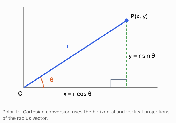
Consider a point P(r, θ).
The coordinates form a right triangle with the horizontal and vertical axes.
Using cosine:
cos θ = x/r
Therefore:
x = r cos θ
Using sine:
sin θ = y/r
Therefore:
y = r sin θ
These formulas work for positive or negative r.
Worked Example 3: Polar to Cartesian
Convert:
P = (6, 30°)
Step 1: Calculate x.
x = 6 cos 30°
x = 6(√3/2)
x = 3√3
Step 2: Calculate y.
y = 6 sin 30°
y = 6(1/2)
y = 3
Answer:
Cartesian coordinates:
(3√3, 3)
Approximately:
(5.20, 3.00)
Worked Example 4: Polar to Cartesian in Another Quadrant
Convert:
Q = (8, 150°)
x = 8 cos 150°
x = −4√3
y = 8 sin 150°
y = 4
Answer: (−4√3, 4)
This is reasonable because an angle of 150° places the point in Quadrant II, where x is negative and y is positive.
Converting Cartesian to Polar
Starting with:
x² + y² = r²
we obtain:
r = √(x² + y²)
For the angle:
tan θ = y/x
However, inverse tangent alone may give the wrong quadrant.
A reliable conversion must use the signs of x and y to determine the correct angle.
Worked Example 5: Cartesian to Polar
Convert:
P = (3, 4)
Step 1: Calculate r.
r = √(3² + 4²)
r = √25
r = 5
Step 2: Calculate θ.
tan θ = 4/3
θ = tan⁻¹(4/3)
θ ≈ 53.13°
Since the point lies in Quadrant I, the angle is correct.
Answer: (5, 53.13°)
Worked Example 6: A Point in Quadrant II
Convert:
Q = (−4, 4)
Step 1: Calculate r.
r = √[(-4)² + 4²]
r = √32
r = 4√2
Step 2: Determine θ.
The reference angle is:
tan⁻¹(|4/−4|) = 45°
Since x is negative and y is positive, the point is in Quadrant II.
θ = 180° − 45°
θ = 135°
Answer: (4√2, 135°)
Worked Example 7: A Point in Quadrant III
Convert:
R = (−5, −5√3)
Radius:
r = √[25 + 75]
r = 10
Reference angle:
α = tan⁻¹(√3) = 60°
The point is in Quadrant III.
θ = 180° + 60°
θ = 240°
Answer: (10, 240°)
Quadrant Reference Guide
|
Quadrant |
Signs of (x, y) |
Angle from reference angle α |
|---|---|---|
|
I |
(+, +) |
θ = α |
|
II |
(−, +) |
θ = 180° − α |
|
III |
(−, −) |
θ = 180° + α |
|
IV |
(+, −) |
θ = 360° − α |
Here α is the acute reference angle, found from the absolute values of x and y.
For points on the coordinate axes, determine the angle directly rather than using inverse tangent.
A Useful Connection to the Unit Circle
For r = 1:
x = cos θ
y = sin θ
The unit circle is therefore a special case of the polar coordinate system.
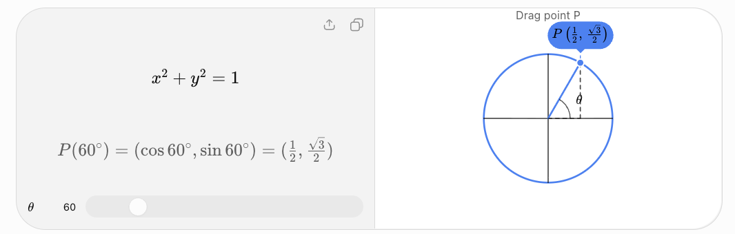
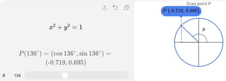
At θ = 60°:
x = cos 60° = 1/2
y = sin 60° = √3/2
So the corresponding Cartesian point is:
(1/2, √3/2)
Learning Target 3: Graphing Simple Polar Equations
In Cartesian coordinates, equations describe relationships between x and y.
In polar coordinates, equations describe relationships between r and θ.
A polar equation may be written as:
r = f(θ)
As θ changes, the value of r determines how far the point lies from the pole.
The resulting points form a curve.
How to Graph a Polar Equation
A useful method is to:
-
Choose several values of θ.
-
Calculate the corresponding values of r.
-
Plot the polar points (r, θ).
-
Connect the points smoothly, following the order of increasing θ.
-
Check whether the graph repeats or has symmetry.
For negative values of r, plot the point in the opposite direction.
Example 8: Graphing r = 3
Consider:
r = 3
The distance from the pole is always 3, regardless of θ.
Therefore, the graph is a circle with:
-
Centre at the pole.
-
Radius 3.
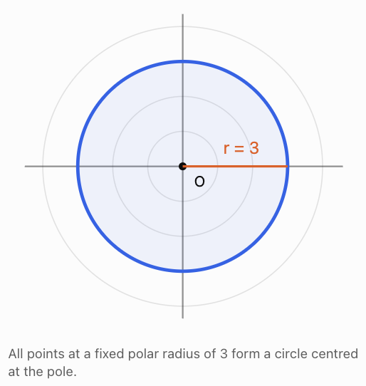 All points at a fixed polar radius of 3 form a circle centred at the pole.
In Cartesian form:
r² = x² + y²
Since r = 3:
x² + y² = 9
This confirms that the graph is a circle of radius 3.
Example 9: Graphing θ = 45°
Consider:
θ = 45°
The angle is fixed, but r can vary.
If r is restricted to nonnegative values, the graph is a ray extending from the pole at 45°.
If r can be any real number, negative radii extend the graph in the opposite direction, producing the complete line through the pole.
Its Cartesian equation is:
y = x
The important distinction is that the domain of r affects whether we obtain a ray or a full line.
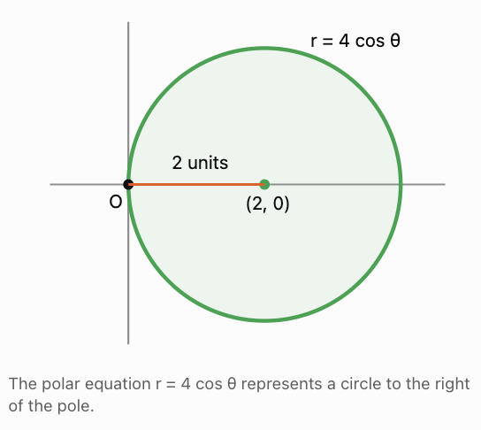
Example 10: Graphing r = 4 cos θ
We can create a table.
θ
r = 4 cos θ
Cartesian point
0°
4
(4, 0)
60°
2
(1, √3)
90°
0
(0, 0)
120°
−2
(1, −√3)
180°
−4
(4, 0)
Notice that negative radii do not mean that the Cartesian x-coordinate must be negative.
At θ = 180°, r = −4 represents the point (4, 0).
To identify the curve, multiply by r:
r² = 4r cos θ
Substitute:
r² = x² + y²
r cos θ = x
Therefore:
x² + y² = 4x
Complete the square:
x² − 4x + y² = 0
(x − 2)² + y² = 4
The graph is a circle with centre (2, 0) and radius 2.
Example 11: Graphing r = 4 sin θ
Multiply by r:
r² = 4r sin θ
Substitute:
x² + y² = 4y
Rearrange:
x² + y² − 4y = 0
Complete the square:
x² + (y − 2)² = 4
This is a circle with:
-
Centre (0, 2).
-
Radius 2.
-
Tangency to the x-axis at the origin.
This provides a useful comparison:
-
r = 4 cos θ gives a circle to the right.
-
r = 4 sin θ gives a circle above the origin.
Example 12: Graphing a Cardioid
Consider:
r = 2(1 + cos θ)
A cardioid is a heart-shaped polar curve with a cusp.
Calculate some values.
θ
r
0°
4
60°
3
90°
2
120°
1
180°
0
240°
1
270°
2
300°
3
360°
4
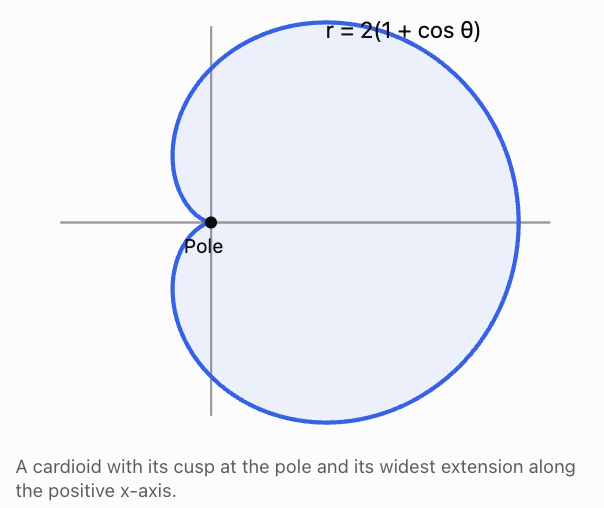
At θ = 0°, r reaches its maximum of 4.
At θ = 180°, r = 0, producing the cusp.
The graph is symmetric about the polar axis because replacing θ with −θ does not change cos θ.
Example 13: Rose Curves
Consider:
r = 3 cos(2θ)
This equation produces a four-petal rose curve.
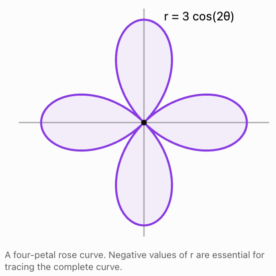
For equations of the form:
r = a cos(nθ)
or:
r = a sin(nθ)
where n is a positive integer:
-
If n is odd, the graph has n petals.
-
If n is even, the graph has 2n petals.
Each petal has maximum distance |a| from the pole.
Example 14: An Archimedean Spiral
Consider:
r = θ, for θ ≥ 0.
As θ increases, the distance from the pole also increases.
The point rotates while moving outward, creating a spiral.
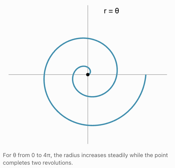
This type of curve is useful in geometric design and in describing idealized spiral motion.
Recognizing Polar Graphs
Polar equation
Typical graph
r = a, a > 0
Circle centred at pole
θ = α
Line through pole if all real r are allowed
r = a cos θ
Circle on horizontal axis
r = a sin θ
Circle on vertical axis
r = a(1 + cos θ)
Cardioid
r = a cos(nθ)
Rose curve
r = aθ
Archimedean spiral
The precise orientation and scale depend on the constants and signs.
Learning Target 4: Interpreting Parametric Equations
What Are Parametric Equations?
A parametric curve describes x and y separately using a third variable called a parameter.
The parameter is often represented by t.
A general parametric representation is:
x = f(t)
y = g(t)
As t changes, the point (x, y) moves along a curve.
The parameter may represent time, an angle, or another quantity.
Unlike an ordinary Cartesian equation, a parametric representation can describe not only the shape of a curve but also the direction in which it is traced.
Worked Example 15: A Straight-Line Path
Consider:
x = 2t + 1
y = 3t − 2
for 0 ≤ t ≤ 3.
Construct a table.
t
x
y
0
1
−2
1
3
1
2
5
4
3
7
7
The point moves from (1, −2) to (7, 7) along a straight line.
To find the Cartesian equation, eliminate t.
From:
x = 2t + 1
t = (x − 1)/2
Substitute into y:
y = 3(x − 1)/2 − 2
y = (3/2)x − 7/2
The Cartesian equation describes the line, while the parameter interval describes the specific segment and its direction of travel.
Worked Example 16: Parametric Equations of a Circle
Consider:
x = 5 cos t
y = 5 sin t
for 0 ≤ t ≤ 2π.
Square both equations:
x² = 25 cos² t
y² = 25 sin² t
Add:
x² + y² = 25(cos² t + sin² t)
Using the identity:
cos² t + sin² t = 1
we obtain:
x² + y² = 25
The curve is a circle of radius 5 centred at the origin.
At t = 0, the point is (5, 0).
At t = π/2, the point is (0, 5).
At t = π, the point is (−5, 0).
At t = 3π/2, the point is (0, −5).
The circle is traced anticlockwise as t increases.
Worked Example 17: Parametric Equations of an Ellipse
Consider:
x = 6 cos t
y = 3 sin t
for 0 ≤ t ≤ 2π.
Divide and square:
x²/36 = cos² t
y²/9 = sin² t
Add:
x²/36 + y²/9 = 1
The curve is an ellipse centred at the origin.
Its horizontal semiaxis is 6 and its vertical semiaxis is 3.
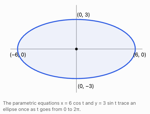
Worked Example 18: Projectile Motion
Parametric equations are especially useful in physics because horizontal and vertical motion can be described separately.
Ignoring air resistance, a projectile launched from the origin at speed v₀ and angle α above the horizontal follows:
x(t) = v₀ cos α × t
y(t) = v₀ sin α × t − ½gt²
where:
-
v₀ is the initial speed.
-
α is the launch angle.
-
g is gravitational acceleration.
-
t is elapsed time.
Suppose a ball is launched at 20 m/s at an angle of 30°.
Take g = 9.8 m/s².
Horizontal motion:
x(t) = 20 cos 30° × t
x(t) = 10√3 t
Vertical motion:
y(t) = 20 sin 30° × t − 4.9t²
y(t) = 10t − 4.9t²
At t = 1 second:
x(1) ≈ 17.32 m
y(1) = 10 − 4.9 = 5.1 m
The ball is approximately 17.32 m horizontally from its starting point and 5.1 m above its launch height.
Interpreting the Parameter
A parametric representation gives more information than the shape of the curve alone.
It can describe:
-
Where a moving object begins.
-
The direction of motion.
-
The speed of motion.
-
Whether the path is traced once or repeatedly.
-
Which part of the curve is included.
For example:
x = cos t, y = sin t
and:
x = cos(2t), y = sin(2t)
describe the same unit circle.
However, over 0 ≤ t ≤ 2π, the first representation traces the circle once, while the second traces it twice.
If t represents time, the second point moves around the circle at twice the angular speed.
Learning Target 5: Connecting Multiple Coordinate Systems
Cartesian, polar, and parametric equations are different ways to represent the same geometric objects.
Understanding the connections allows us to choose the most useful representation for a particular problem.
Three Representations of a Circle
Consider a circle of radius 4 centred at the origin.
Cartesian form:
x² + y² = 16
Polar form:
r = 4
Parametric form:
x = 4 cos t
y = 4 sin t
for 0 ≤ t ≤ 2π.
All three describe the same circle.
However, each emphasizes different information.
-
Cartesian form expresses a relationship between x and y.
-
Polar form emphasizes constant distance from the origin.
-
Parametric form describes how a point travels around the circle.
Worked Example 19: Converting a Polar Equation to Cartesian Form
Convert:
r = 6 cos θ
Multiply by r:
r² = 6r cos θ
Substitute:
r² = x² + y²
r cos θ = x
Therefore:
x² + y² = 6x
Complete the square:
x² − 6x + y² = 0
(x − 3)² + y² = 9
Cartesian equation: (x − 3)² + y² = 9
The curve is a circle with centre (3, 0) and radius 3.
Worked Example 20: Converting Cartesian to Polar Form
Convert:
x² + y² = 8y
Use:
x² + y² = r²
y = r sin θ
Therefore:
r² = 8r sin θ
For r ≠ 0:
r = 8 sin θ
The pole r = 0 also satisfies both equations, so it is included in the curve.
Polar equation: r = 8 sin θ
The graph is a circle with centre (0, 4) and radius 4.
Worked Example 21: Connecting Polar and Parametric Equations
Consider the polar curve:
r = 2 + cos θ
We know:
x = r cos θ
y = r sin θ
Substitute the expression for r:
x = (2 + cos θ)cos θ
y = (2 + cos θ)sin θ
Let the parameter t = θ.
Then:
x(t) = (2 + cos t)cos t
y(t) = (2 + cos t)sin t
for 0 ≤ t ≤ 2π.
These parametric equations describe the same curve as the polar equation.
The curve is a limacon, with no inner loop because r remains positive.
Worked Example 22: Converting a Parametric Curve to Polar Form
Consider:
x = 3t cos t
y = 3t sin t
for t ≥ 0.
Calculate r:
r = √(x² + y²)
r = √(9t²cos²t + 9t²sin²t)
r = √(9t²)
Since t ≥ 0:
r = 3t
The angle of the point is:
θ = t, modulo 2π.
Using the continuous angle parameter θ = t:
r = 3θ, for θ ≥ 0.
This is an Archimedean spiral.
The parameter t describes both the rotation and the increasing distance from the origin.
Choosing the Most Useful Coordinate System
Situation
Useful representation
Reason
Straight lines and standard function graphs
Cartesian
Direct x-y relationships
Circular motion around a centre
Polar or parametric
Radius and angle are natural
Radar location
Polar
Distance and direction are measured
Projectile motion
Parametric
Coordinates change with time
Spiral curves
Polar
Radius depends on angle
Ellipses traced by moving points
Parametric
Easy to describe using sine and cosine
Intersections of algebraic curves
Cartesian
Algebraic methods are often convenient
No coordinate system is universally best.
The most effective representation depends on the geometry, the given information, and the purpose of the calculation.
Real-World Applications
Radar and Navigation
Radar systems often measure the distance and direction of an object relative to a fixed station.
These are naturally polar measurements.
For example, an aircraft located 50 km away at a standard polar angle of 35° has Cartesian coordinates:
x = 50 cos 35° ≈ 40.96 km
y = 50 sin 35° ≈ 28.68 km
The aircraft is approximately 40.96 km east and 28.68 km north of the station, assuming the positive axes represent east and north.
If the direction is instead given as a compass bearing, the angle convention must first be converted.
Computer Graphics and Animation
Parametric equations are widely used to animate moving objects.
A point moving around a circle may be represented by:
x(t) = 100 cos t
y(t) = 100 sin t
The point moves around a circle of radius 100 units.
Changing the coefficient of t changes the angular speed.
Robotics
A robot arm rotating around a fixed joint can be modelled using:
x = L cos θ
y = L sin θ
where L is the arm length.
For a 2 m arm rotated to 60°:
x = 2 cos 60° = 1 m
y = 2 sin 60° = √3 m
This allows engineers to calculate the position of the arm's endpoint.
Astronomy
Polar coordinates are useful for describing positions relative to a central body.
For example, the orbit of an object under an ideal inverse-square gravitational force can be expressed in polar form, with the central body at a focus:
r = p/(1 + e cos θ)
where p is a length parameter and e is eccentricity.
For 0 ≤ e < 1, this describes an ellipse; e = 0 gives a circle.
Physics and Engineering
Parametric equations can describe:
-
Projectile trajectories.
-
Circular and elliptical motion.
-
Oscillations.
-
Paths of moving machinery.
-
Fluid particle trajectories.
They are particularly useful when the horizontal and vertical coordinates depend on time.
Common Mistakes
Mistake 1: Measuring Polar Angles from North
Standard polar angles are measured from the positive x-axis, usually anticlockwise.
Compass bearings use a different convention.
Mistake 2: Assuming Polar Coordinates Are Unique
A point may have infinitely many polar representations.
For example:
(3, 45°) and (3, 405°) represent the same point.
Mistake 3: Ignoring Negative Radii
A negative radius reverses the direction of the point.
For example:
(−5, 30°) = (5, 210°)
Mistake 4: Using the Wrong Quadrant
When converting Cartesian coordinates to polar form, inverse tangent alone may not give the correct angle.
Always examine the signs of x and y.
Mistake 5: Confusing x = r cos θ and y = r sin θ
Cosine gives the horizontal component.
Sine gives the vertical component.
Mistake 6: Forgetting the Parameter Interval
Parametric equations may describe only part of a curve.
For example:
x = cos t, y = sin t, 0 ≤ t ≤ π
traces the upper semicircle, not the full circle.
Mistake 7: Ignoring the Direction of a Parametric Curve
The parameter determines how the curve is traced.
Two parameterizations may have the same geometric graph but opposite directions.
Mistake 8: Losing Points When Dividing by r
When converting polar equations, dividing by r may exclude the pole.
Always check separately whether r = 0 satisfies the original equation.
Mistake 9: Using Degrees in a Radian-Based Formula
Most calculus and parametric formulas use radians.
Check the angle units before calculating.
Mistake 10: Assuming Every Curve Is a Function y = f(x)
A circle cannot be represented by one single-valued function y = f(x) over its full horizontal extent.
Polar and parametric representations can describe such curves naturally.
Key Terms
-
Cartesian coordinates: Coordinates (x, y) describing horizontal and vertical position.
-
Polar coordinates: Coordinates (r, θ) describing directed distance and angle.
-
Pole: The origin of the polar coordinate system.
-
Polar axis: The reference direction from which polar angles are measured.
-
Radius: The directed distance r used in polar coordinates.
-
Polar angle: The angular coordinate θ.
-
Reference angle: An acute angle used to determine trigonometric values and coordinate quadrants.
-
Quadrant: One of the four regions formed by the Cartesian axes.
-
Polar equation: An equation relating r and θ.
-
Parametric equation: An equation expressing a coordinate in terms of a parameter.
-
Parameter: A variable used to describe points on a curve.
-
Parameterization: A representation of a curve using one or more parameter-dependent coordinates.
-
Circle: The set of points at a fixed distance from a centre.
-
Ellipse: A closed curve characterized by two focal points.
-
Cardioid: A heart-shaped polar curve with a cusp.
-
Limacon: A family of polar curves that may have an inner loop, dimple, or convex shape.
-
Rose curve: A polar curve with petal-like loops.
-
Archimedean spiral: A spiral whose radius changes linearly with its angle.
-
Coordinate transformation: A conversion between coordinate systems.
-
Eliminating a parameter: Rewriting parametric equations as a direct relationship between x and y.
-
Trajectory: The path followed by a moving object.
-
Angular speed: The rate of change of angle with respect to time.
Key Takeaways
-
Polar coordinates describe a point using a directed radius and an angle.
-
The standard polar angle is measured anticlockwise from the positive x-axis.
-
Polar coordinates are not unique.
-
The conversion formulas are x = r cos θ and y = r sin θ.
-
For the usual nonnegative-radius representation, r = √(x² + y²).
-
The angle must be selected using the correct quadrant.
-
Polar equations can represent circles, cardioids, rose curves, and spirals.
-
Parametric equations describe x and y using a common parameter.
-
The parameter can describe motion, direction, speed, and the portion of a curve traced.
-
Cartesian, polar, and parametric forms can represent the same geometric curve.
-
Choosing an appropriate coordinate system can simplify mathematical problems.
-
These coordinate systems are important in navigation, physics, engineering, robotics, and computer graphics.
Check Your Understanding
Part A: Polar Coordinates
Question 1
Explain the meaning of each polar coordinate pair.
a) (5, 30°)
b) (4, 135°)
c) (−3, 60°)
Question 2
Write two other polar representations of the point (6, 45°).
Part B: Coordinate Conversion
Question 3
Convert the following polar coordinates into Cartesian coordinates.
a) (4, 60°)
b) (6, 180°)
c) (8, 225°)
Question 4
Convert the following Cartesian coordinates into polar coordinates with r ≥ 0 and 0° ≤ θ < 360°.
a) (3, 3)
b) (−5, 0)
c) (−4, −4)
Part C: Polar Graphs
Question 5
Describe the graph of:
r = 5
Question 6
Convert the following polar equation into Cartesian form and identify the curve.
r = 6 cos θ
Question 7
Explain why:
r = 2(1 + cos θ)
has a cusp at the pole.
Part D: Parametric Equations
Question 8
Given:
x = 3t + 2
y = 2t − 1
a) Find the point when t = 4.
b) Eliminate t to obtain a Cartesian equation.
Question 9
Consider:
x = 4 cos t
y = 4 sin t
for 0 ≤ t ≤ 2π.
a) Identify the curve.
b) State its radius.
c) Describe its direction of travel.
Question 10
Given:
x = 5 cos t
y = 2 sin t
eliminate the parameter and identify the curve.
Part E: Connecting Coordinate Systems
Question 11
Convert the Cartesian equation:
x² + y² = 10x
into polar form.
Question 12
A point moves according to:
x = 2t cos t
y = 2t sin t
for t ≥ 0.
a) Find its polar radius.
b) Describe its angle.
c) Identify the resulting curve.
Check Your Understanding — Fully Worked Answers
Answer 1
a) (5, 30°)
Move 5 units from the pole at an angle of 30° anticlockwise from the positive x-axis.
b) (4, 135°)
Move 4 units from the pole in the direction 135°, placing the point in Quadrant II.
c) (−3, 60°)
The negative radius means moving 3 units opposite the direction 60°.
Equivalent positive-radius coordinates:
(3, 240°)
Answer 2
Adding 360°:
(6, 45° + 360°) = (6, 405°)
Using a negative radius:
(−6, 45° + 180°) = (−6, 225°)
Answers: (6, 405°) and (−6, 225°)
Answer 3
a) (4, 60°)
x = 4 cos 60° = 2
y = 4 sin 60° = 2√3
Answer: (2, 2√3)
b) (6, 180°)
x = 6 cos 180° = −6
y = 6 sin 180° = 0
Answer: (−6, 0)
c) (8, 225°)
x = 8 cos 225° = −4√2
y = 8 sin 225° = −4√2
Answer: (−4√2, −4√2)
Answer 4
a) (3, 3)
r = √(9 + 9) = 3√2
θ = 45°
Answer: (3√2, 45°)
b) (−5, 0)
r = 5
The point lies on the negative x-axis.
θ = 180°
Answer: (5, 180°)
c) (−4, −4)
r = √(16 + 16) = 4√2
The reference angle is 45°.
The point is in Quadrant III.
θ = 225°
Answer: (4√2, 225°)
Answer 5
The equation r = 5 represents all points at a distance of 5 units from the pole.
The graph is a circle of radius 5 centred at the origin.
Its Cartesian equation is:
x² + y² = 25
Answer 6
Given:
r = 6 cos θ
Multiply by r:
r² = 6r cos θ
Substitute:
x² + y² = 6x
Complete the square:
x² − 6x + y² = 0
(x − 3)² + y² = 9
This is a circle with centre (3, 0) and radius 3.
Answer 7
Given:
r = 2(1 + cos θ)
At θ = 180°:
cos 180° = −1
Therefore:
r = 2(1 − 1) = 0
The curve reaches the pole at θ = 180°.
The two branches meet there, producing a cusp.
Answer 8
Given:
x = 3t + 2
y = 2t − 1
a) At t = 4
x = 3(4) + 2 = 14
y = 2(4) − 1 = 7
Answer: (14, 7)
b) Eliminate t
From x = 3t + 2:
t = (x − 2)/3
Substitute into y:
y = 2(x − 2)/3 − 1
y = (2x − 4)/3 − 1
y = (2x − 7)/3
Answer 9
Given:
x = 4 cos t
y = 4 sin t
Square and add:
x² + y² = 16(cos²t + sin²t)
x² + y² = 16
a) The curve is a circle centred at the origin.
b) Radius = 4 units.
c) The circle is traced anticlockwise as t increases from 0 to 2π, starting at (4, 0).
Answer 10
Given:
x = 5 cos t
y = 2 sin t
Divide:
x/5 = cos t
y/2 = sin t
Square and add:
x²/25 + y²/4 = cos²t + sin²t
x²/25 + y²/4 = 1
The curve is an ellipse centred at the origin with horizontal semiaxis 5 and vertical semiaxis 2.
Answer 11
Given:
x² + y² = 10x
Substitute:
x² + y² = r²
x = r cos θ
Therefore:
r² = 10r cos θ
For r ≠ 0:
r = 10 cos θ
The pole is also included.
Answer: r = 10 cos θ
Answer 12
Given:
x = 2t cos t
y = 2t sin t
for t ≥ 0.
a) Calculate the radius.
r = √(x² + y²)
r = √(4t²cos²t + 4t²sin²t)
r = √(4t²)
Since t ≥ 0:
r = 2t
b) Determine the angle.
The polar angle is t modulo 2π.
Using a continuous angle:
θ = t
c) Identify the curve.
Substitute t = θ:
r = 2θ
The curve is an Archimedean spiral.
Final Integrated Challenge: Designing a Robotic Tracking System
A robot moves around a central observation station.
Its distance from the station depends on its angle according to:
r = 4 + 2 cos θ
where r is measured in metres and 0 ≤ θ ≤ 2π.
Tasks
-
Explain what the polar equation represents.
-
Determine the maximum and minimum distances from the station.
-
Calculate the robot's Cartesian coordinates at θ = 0, π/2, π, and 3π/2.
-
Write parametric equations for its motion.
-
Explain why this curve is easier to represent in polar coordinates than in Cartesian coordinates.
-
Evaluate whether the model describes constant-speed motion.
Fully Worked Solution
Step 1: Interpret the polar equation.
The robot's distance from the observation station changes according to its angular position.
The radius is:
r = 4 + 2 cos θ
Since cos θ varies between −1 and 1:
2 ≤ r ≤ 6
The robot follows a closed limacon-shaped path without an inner loop.
Step 2: Find the maximum distance.
The maximum occurs when cos θ = 1.
r(max) = 4 + 2(1)
Maximum distance = 6 m
Step 3: Find the minimum distance.
The minimum occurs when cos θ = −1.
r(min) = 4 + 2(−1)
Minimum distance = 2 m
Step 4: Calculate Cartesian coordinates.
Use:
x = r cos θ
y = r sin θ
θ
r
x
y
0
6
6
0
π/2
4
0
4
π
2
−2
0
3π/2
4
0
−4
These points show that the curve extends farther to the right than to the left.
Step 5: Construct parametric equations.
Let t = θ.
Then:
r = 4 + 2 cos t
Substitute into the coordinate conversion formulas:
x(t) = (4 + 2 cos t)cos t
y(t) = (4 + 2 cos t)sin t
for 0 ≤ t ≤ 2π.
Step 6: Compare coordinate systems.
The polar equation is compact:
r = 4 + 2 cos θ
The parametric representation requires two equations.
A Cartesian equation can also be derived, but it is more complicated.
Using:
r = √(x² + y²)
cos θ = x/r
we obtain:
r = 4 + 2x/r
Multiply by r:
r² = 4r + 2x
Therefore:
x² + y² = 4√(x² + y²) + 2x
This implicit Cartesian equation represents the same curve, but the polar form is easier to interpret.
Step 7: Evaluate the motion.
The parametric equations describe the path and the direction in which it is traced.
However, the model does not automatically imply constant speed.
If t represents time and θ = t, then angular speed is constant, but the radius changes.
The speed depends on both the radial change and angular motion.
For r = 4 + 2 cos t:
dr/dt = −2 sin t
With dθ/dt = 1 rad/s, speed is:
v = √[(dr/dt)² + (r dθ/dt)²]
v = √[4 sin²t + (4 + 2 cos t)²]
This expression changes with t.
Therefore, the robot does not move at constant speed under this time parameterization.
Final Challenge Summary
Property
Result
Polar equation
r = 4 + 2 cos θ
Curve type
Limacon without inner loop
Maximum radius
6 m
Minimum radius
2 m
Rightmost point
(6, 0)
Leftmost point
(−2, 0)
Upper-axis point
(0, 4)
Lower-axis point
(0, −4)
Constant speed when θ = t?
No
Conclusion
Polar coordinates and parametric curves extend coordinate geometry beyond the familiar Cartesian system.
Polar coordinates describe locations using distance and direction, making them especially useful for circular motion, radar tracking, spirals, and other rotational patterns.
The conversion formulas allow us to move between polar and Cartesian representations, while careful attention to quadrants and negative radii ensures that coordinates are interpreted correctly.
Polar equations provide elegant descriptions of circles, cardioids, rose curves, and spirals.
Parametric equations offer another powerful perspective by expressing x and y in terms of a shared parameter. This makes it possible to describe not only the shape of a curve but also how a point moves along it.
By connecting Cartesian, polar, and parametric systems, we gain flexibility in solving mathematical problems and modelling physical situations.
The most important skill is recognizing which coordinate system best represents the geometry or motion being studied, and understanding how to translate between different representations of the same mathematical relationship.
-
3. Complex Numbers and Trigonometry
Learning outcomes
- I can represent complex numbers in polar form.
- I can relate trigonometry to complex numbers.
- I can perform operations using polar form.
- I can interpret geometric representations of complex numbers.
- I can solve problems involving polar representations.
Introduction
Complex numbers and trigonometry are closely connected. Together, they provide a powerful way to describe rotation, magnitude, direction, and periodic behaviour.
A complex number such as:
z = 3 + 4i
can be interpreted algebraically as a sum of real and imaginary components. However, it can also be represented geometrically as a point in a coordinate plane.
This geometric interpretation reveals an important connection: a complex number can be described using its distance from the origin and its angle with the positive real axis.
These are the same ideas used in polar coordinates and trigonometry.
By expressing complex numbers in polar form, operations such as multiplication, division, powers, and roots become easier to understand and often simpler to calculate.
For example, multiplying two complex numbers can be interpreted as combining their magnitudes and adding their angles. Raising a complex number to a power becomes a process of raising its magnitude to that power and multiplying its angle.
These relationships are useful in mathematics, physics, electrical engineering, signal processing, computer graphics, and the study of rotations.
In this lesson, we will explore the connection between complex numbers and trigonometry, convert between rectangular and polar forms, perform operations using polar form, interpret complex numbers geometrically, and solve practical problems involving complex-number representations.
Understanding Complex Numbers
Rectangular Form
A complex number is usually written as:
z = a + bi
where:
-
a is the real part.
-
b is the imaginary part.
-
i is the imaginary unit, defined by i² = −1.
For example:
z = 5 + 2i
has:
Real part = 5
Imaginary part = 2
Another example:
z = −3 + 4i
has:
Real part = −3
Imaginary part = 4
The real and imaginary components can be represented on a coordinate plane.
The Complex Plane
The complex plane, also called the Argand plane, uses:
-
A horizontal real axis.
-
A vertical imaginary axis.
A complex number z = a + bi corresponds to the point (a, b).
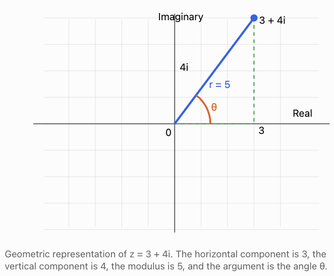
This diagram reveals two important quantities:
-
The distance of the point from the origin.
-
The angle the point makes with the positive real axis.
These lead directly to the polar form of a complex number.
Learning Target 1: Representing Complex Numbers in Polar Form
The Modulus of a Complex Number
The modulus of a complex number is its distance from the origin in the complex plane.
For:
z = a + bi
the modulus is:
|z| = √(a² + b²)
The modulus is always nonnegative.
Worked Example 1: Calculating the Modulus
Find the modulus of:
z = 6 + 8i
Step 1: Identify the components.
a = 6
b = 8
Step 2: Apply the modulus formula.
|z| = √(6² + 8²)
|z| = √(36 + 64)
|z| = √100
|z| = 10
Geometrically, the point (6, 8) lies 10 units from the origin.
The Argument of a Complex Number
The argument is the angle measured anticlockwise from the positive real axis to the line joining the origin to the complex number.
It is represented by:
arg(z) = θ
For z ≠ 0, we can use:
tan θ = b/a
when a ≠ 0.
However, inverse tangent must be interpreted using the correct quadrant.
For example, a point with negative real and positive imaginary parts lies in Quadrant II.
A calculator's inverse tangent may return a negative acute angle, so the quadrant must be considered.
The Principal Argument
A nonzero complex number has infinitely many possible arguments because full revolutions do not change its direction.
If θ is an argument, then:
θ + 2πk
is also an argument, where k is any integer.
The principal argument, written Arg(z), is commonly chosen in the interval:
−π < Arg(z) ≤ π
Some textbooks use a different convention, such as 0 ≤ θ < 2π. Both are valid if used consistently.
The complex number zero has no defined argument.
Worked Example 2: Finding the Argument
Find the argument of:
z = 3 + 3i
The point is in Quadrant I.
tan θ = 3/3 = 1
θ = 45° = π/4
Arg(z) = π/4
Worked Example 3: Argument in Quadrant II
Find the principal argument of:
z = −4 + 4i
The point is in Quadrant II.
The reference angle is:
α = tan⁻¹(4/4) = 45°
Therefore:
θ = 180° − 45°
Arg(z) = 135° = 3π/4
Deriving Polar Form
Consider a complex number:
z = a + bi
Let its modulus be r and its argument be θ.
From trigonometry:
a = r cos θ
b = r sin θ
Substitute into rectangular form:
z = r cos θ + i(r sin θ)
Factor out r:
z = r(cos θ + i sin θ)
This is the polar form, also called the trigonometric form, of a complex number.
For z ≠ 0, r > 0 and θ may be any argument of z.
Worked Example 4: Rectangular to Polar Form
Convert:
z = 3 + 4i
Step 1: Find the modulus.
r = √(3² + 4²)
r = 5
Step 2: Find the argument.
tan θ = 4/3
θ ≈ 53.13°
Step 3: Write the polar form.
z = 5(cos 53.13° + i sin 53.13°)
Using radians:
z ≈ 5(cos 0.9273 + i sin 0.9273)
Worked Example 5: Polar to Rectangular Form
Convert:
z = 8(cos 150° + i sin 150°)
Use:
cos 150° = −√3/2
sin 150° = 1/2
Therefore:
z = 8(−√3/2 + i/2)
z = −4√3 + 4i
Using the cis Notation
To simplify repeated expressions, mathematicians sometimes use:
cis θ = cos θ + i sin θ
Therefore:
z = r cis θ
For example:
5(cos 60° + i sin 60°)
can be written:
5 cis 60°
The cis notation is especially useful for multiplication, division, powers, and roots.
Special Cases
|
Complex number |
Modulus |
Principal argument |
|---|---|---|
|
5 |
5 |
0 |
|
4i |
4 |
π/2 |
|
−6 |
6 |
π |
|
−3i |
3 |
−π/2 |
|
1 + i |
√2 |
π/4 |
|
−1 + i |
√2 |
3π/4 |
|
−1 − i |
√2 |
−3π/4 |
|
1 − i |
√2 |
−π/4 |
For z = 0, the modulus is 0 but the argument is undefined.
Learning Target 2: Relating Trigonometry to Complex Numbers
The Unit Circle Connection
A complex number with modulus 1 lies on the unit circle.
For r = 1:
z = cos θ + i sin θ
The real part is cos θ and the imaginary part is sin θ.
This is exactly the same relationship used in trigonometry and polar coordinates.
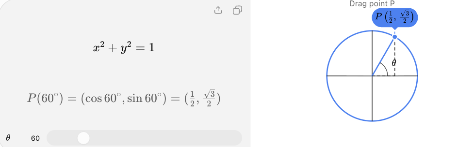
For θ = 60°:
cos 60° = 1/2
sin 60° = √3/2
Therefore, the corresponding complex number is:
z = 1/2 + (√3/2)i
Its modulus is:
|z| = √(1/4 + 3/4) = 1
Euler's Formula
One of the most important relationships in mathematics is Euler's formula:
e^(iθ) = cos θ + i sin θ
Here θ is measured in radians.
This allows polar form to be written as:
z = re^(iθ)
For example:
z = 5(cos π/3 + i sin π/3)
can be written:
z = 5e^(iπ/3)
Euler's formula connects exponential functions, complex numbers, and trigonometry.
Why Euler's Formula Matters
Euler's formula makes complex multiplication especially elegant.
Consider:
z₁ = r₁e^(iθ₁)
z₂ = r₂e^(iθ₂)
Multiplying:
z₁z₂ = r₁r₂e^[i(θ₁ + θ₂)]
This shows that multiplying complex numbers:
-
Multiplies their moduli.
-
Adds their arguments.
Geometrically, multiplication combines scaling and rotation.
Euler's Identity
Setting θ = π in Euler's formula gives:
e^(iπ) = cos π + i sin π
e^(iπ) = −1
Therefore:
e^(iπ) + 1 = 0
This famous identity connects five fundamental mathematical constants:
e, i, π, 1, and 0.
Complex Conjugates and Trigonometry
The complex conjugate of:
z = a + bi
is:
z̄ = a − bi
In polar form:
z = r(cos θ + i sin θ)
Its conjugate is:
z̄ = r(cos θ − i sin θ)
Since cosine is even and sine is odd:
z̄ = r[cos(−θ) + i sin(−θ)]
Thus, conjugation changes the sign of the argument.
Geometrically, this reflects the complex number across the real axis.
Worked Example 6: Conjugate in Polar Form
Given:
z = 6 cis 40°
Find its conjugate.
The modulus remains 6.
The argument changes from 40° to −40°.
z̄ = 6 cis(−40°)
Modulus of a Product
For any complex numbers z₁ and z₂:
|z₁z₂| = |z₁||z₂|
This is consistent with the multiplication rule in polar form.
For example, if:
|z₁| = 3
|z₂| = 5
then:
|z₁z₂| = 15
regardless of their arguments.
Learning Target 3: Performing Operations Using Polar Form
Polar form is particularly useful for multiplication, division, powers, and roots.
Addition and subtraction are usually easier in rectangular form.
Multiplying Complex Numbers
Suppose:
z₁ = r₁ cis θ₁
z₂ = r₂ cis θ₂
Then:
z₁z₂ = r₁r₂ cis(θ₁ + θ₂)
This means:
-
Multiply the moduli.
-
Add the arguments.
Why Does This Rule Work?
Start with:
z₁z₂ = r₁(cos θ₁ + i sin θ₁) × r₂(cos θ₂ + i sin θ₂)
Expand:
z₁z₂ = r₁r₂[(cos θ₁ cos θ₂ − sin θ₁ sin θ₂) + i(sin θ₁ cos θ₂ + cos θ₁ sin θ₂)]
Using the trigonometric addition identities:
cos(θ₁ + θ₂) = cos θ₁ cos θ₂ − sin θ₁ sin θ₂
sin(θ₁ + θ₂) = sin θ₁ cos θ₂ + cos θ₁ sin θ₂
Therefore:
z₁z₂ = r₁r₂[cos(θ₁ + θ₂) + i sin(θ₁ + θ₂)]
This establishes the multiplication rule.
Worked Example 7: Multiplication in Polar Form
Calculate:
z₁ = 4 cis 30°
z₂ = 3 cis 70°
Step 1: Multiply the moduli.
4 × 3 = 12
Step 2: Add the arguments.
30° + 70° = 100°
Answer:
z₁z₂ = 12 cis 100°
The resulting complex number has modulus 12 and argument 100°.
Worked Example 8: Multiplication with an Argument Greater Than 360°
Calculate:
(5 cis 250°)(2 cis 160°)
Multiply the moduli:
5 × 2 = 10
Add the arguments:
250° + 160° = 410°
Therefore:
z = 10 cis 410°
Since 410° − 360° = 50°:
z = 10 cis 50°
Both expressions represent the same complex number.
Dividing Complex Numbers
For z₂ ≠ 0:
z₁/z₂ = (r₁/r₂) cis(θ₁ − θ₂)
This means:
-
Divide the moduli.
-
Subtract the arguments.
Worked Example 9: Division in Polar Form
Calculate:
z₁ = 18 cis 130°
z₂ = 3 cis 40°
Step 1: Divide the moduli.
18/3 = 6
Step 2: Subtract the arguments.
130° − 40° = 90°
Answer:
z₁/z₂ = 6 cis 90°
Since cos 90° = 0 and sin 90° = 1:
z₁/z₂ = 6i
Worked Example 10: Division with a Negative Argument
Calculate:
(20 cis 25°)/(4 cis 100°)
Divide the moduli:
20/4 = 5
Subtract the arguments:
25° − 100° = −75°
Answer: 5 cis(−75°)
An equivalent positive argument is 285°.
Powers of Complex Numbers: De Moivre's Theorem
Repeated multiplication leads to an important theorem.
If:
z = r(cos θ + i sin θ)
then, for any integer n:
zⁿ = rⁿ[cos(nθ) + i sin(nθ)]
This is De Moivre's theorem.
It also works for negative integers when z ≠ 0.
In cis notation:
(r cis θ)ⁿ = rⁿ cis(nθ)
To raise a complex number to a power:
-
Raise the modulus to that power.
-
Multiply the argument by the power.
Worked Example 11: Calculating a Power
Calculate:
(2 cis 30°)⁴
Apply De Moivre's theorem.
Modulus:
2⁴ = 16
Argument:
4 × 30° = 120°
Therefore:
z⁴ = 16 cis 120°
Convert to rectangular form:
z⁴ = 16(cos 120° + i sin 120°)
z⁴ = 16(−1/2 + i√3/2)
z⁴ = −8 + 8√3i
Worked Example 12: Evaluating (1 + i)⁸
Step 1: Convert to polar form.
For z = 1 + i:
r = √(1² + 1²) = √2
θ = 45°
Therefore:
z = √2 cis 45°
Step 2: Apply De Moivre's theorem.
z⁸ = (√2)⁸ cis(8 × 45°)
z⁸ = 16 cis 360°
Step 3: Convert to rectangular form.
cos 360° = 1
sin 360° = 0
(1 + i)⁸ = 16
This calculation is much shorter than multiplying 1 + i by itself eight times.
Roots of Complex Numbers
Finding roots reverses the process of raising a complex number to a power.
Suppose:
wⁿ = z
where:
z = r cis θ
For z ≠ 0, the n distinct complex nth roots are:
wₖ = r^(1/n) cis[(θ + 360°k)/n]
where:
k = 0, 1, 2, ..., n − 1
In radians:
wₖ = r^(1/n) cis[(θ + 2πk)/n]
The different values of k account for all possible arguments.
Why Are There n Roots?
If w has modulus s and argument φ, then:
wⁿ = sⁿ cis(nφ)
For wⁿ = r cis θ:
sⁿ = r
and:
nφ = θ + 360°k
Therefore:
s = r^(1/n)
φ = (θ + 360°k)/n
There are n distinct angles before the pattern repeats.
Worked Example 13: Finding the Cube Roots of 8
Solve:
z³ = 8
Write 8 in polar form:
8 = 8 cis 0°
The cube-root modulus is:
r = ∛8 = 2
The arguments are:
θₖ = (0° + 360°k)/3
For k = 0:
θ₀ = 0°
For k = 1:
θ₁ = 120°
For k = 2:
θ₂ = 240°
Therefore, the three roots are:
z₀ = 2 cis 0° = 2
z₁ = 2 cis 120° = −1 + √3i
z₂ = 2 cis 240° = −1 − √3i
Final answers:
-
2
-
−1 + √3i
-
−1 − √3i
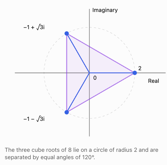
Worked Example 14: Finding Fourth Roots
Solve:
z⁴ = −16
Write:
−16 = 16 cis 180°
The root modulus is:
r = 16^(1/4) = 2
The arguments are:
θₖ = (180° + 360°k)/4
For k = 0, 1, 2, 3:
-
θ₀ = 45°
-
θ₁ = 135°
-
θ₂ = 225°
-
θ₃ = 315°
Therefore:
z = 2 cis 45°, 2 cis 135°, 2 cis 225°, or 2 cis 315°
In rectangular form:
-
√2 + √2i
-
−√2 + √2i
-
−√2 − √2i
-
√2 − √2i
The four roots form the vertices of a square centred at the origin.
Addition and Subtraction
Polar form is usually less convenient for addition and subtraction.
For example:
z₁ = 4 cis 0° = 4
z₂ = 4 cis 90° = 4i
Their sum is:
z₁ + z₂ = 4 + 4i
Converting back to polar form:
r = √(4² + 4²) = 4√2
θ = 45°
Therefore:
z₁ + z₂ = 4√2 cis 45°
Notice that we did not add the moduli and arguments. That rule applies to multiplication, not addition.
Operations Summary
Operation
Polar-form rule
Multiplication
Multiply moduli; add arguments
Division
Divide moduli; subtract arguments
Integer powers
Raise modulus to power; multiply argument
nth roots
Take nth root of modulus; divide all possible arguments by n
Addition
Usually convert to rectangular form
Subtraction
Usually convert to rectangular form
Conjugation
Keep modulus; negate argument
Learning Target 4: Interpreting Geometric Representations of Complex Numbers
Complex numbers are not only algebraic expressions. They also represent vectors, rotations, reflections, and transformations.
Complex Numbers as Vectors
A complex number:
z = a + bi
can be represented by a vector from the origin to the point (a, b).
Its modulus represents the vector's length.
Its argument represents the vector's direction.
For example:
z = 3 + 4i
corresponds to a vector with:
-
Horizontal component = 3
-
Vertical component = 4
-
Length = 5
-
Direction ≈ 53.13° from the positive real axis
Addition as Vector Addition
Consider:
z₁ = 3 + 2i
z₂ = 1 + 3i
Add the real components:
3 + 1 = 4
Add the imaginary components:
2i + 3i = 5i
Therefore:
z₁ + z₂ = 4 + 5i
Geometrically, the two vectors can be added using the parallelogram or head-to-tail method.
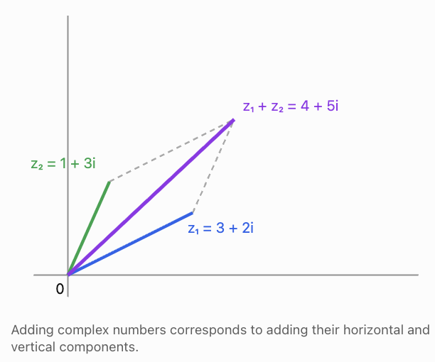
Multiplication as Rotation and Scaling
Multiplication has a different geometric meaning.
Suppose:
z = r cis θ
and:
w = s cis φ
Then:
zw = rs cis(θ + φ)
Multiplication by w:
-
Scales the distance from the origin by s.
-
Rotates the point anticlockwise by φ.
If s = 1, the transformation is a pure rotation.
If φ = 0°, the transformation is a pure scaling by a positive factor.
Worked Example 15: Rotation by 90°
Consider:
z = 3 + 2i
Multiply by i.
iz = i(3 + 2i)
iz = 3i + 2i²
Since i² = −1:
iz = −2 + 3i
The original point is (3, 2).
The new point is (−2, 3).
This is a 90° anticlockwise rotation about the origin.
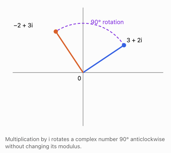
Rotating by Any Angle
To rotate a complex number by an angle α anticlockwise, multiply it by:
cos α + i sin α
or:
cis α
For example, to rotate z by 60°:
z(new) = z cis 60°
Because cis 60° has modulus 1, the distance from the origin does not change.
Worked Example 16: Rotation and Scaling Together
A point is represented by:
z = 2 cis 30°
It is transformed by multiplying by:
w = 3 cis 45°
Find the new position.
Step 1: Multiply the moduli.
2 × 3 = 6
Step 2: Add the angles.
30° + 45° = 75°
Therefore:
zw = 6 cis 75°
The transformation triples the point's distance from the origin and rotates it 45° anticlockwise.
Reflection Across the Real Axis
The complex conjugate reflects a point across the real axis.
For example:
z = 2 + 5i
z̄ = 2 − 5i
The point (2, 5) becomes (2, −5).
The modulus remains unchanged, while the argument changes sign.
Reflection Across the Imaginary Axis
To reflect z = a + bi across the imaginary axis:
a + bi → −a + bi
This can be expressed as:
z(new) = −z̄
For example:
z = 3 + 4i
z̄ = 3 − 4i
−z̄ = −3 + 4i
The point (3, 4) becomes (−3, 4).
Distance Between Complex Numbers
If z₁ and z₂ represent two points, their distance is:
d = |z₂ − z₁|
This is the same as the Cartesian distance formula.
Worked Example 17: Distance in the Complex Plane
Find the distance between:
z₁ = 2 + 3i
z₂ = 7 − i
Subtract:
z₂ − z₁ = (7 − i) − (2 + 3i)
z₂ − z₁ = 5 − 4i
Calculate the modulus:
d = √(5² + (−4)²)
d = √41 ≈ 6.40 units
Geometric Loci
A locus is the set of points satisfying a given condition.
Complex notation can describe geometric loci concisely.
For example:
|z − (2 + 3i)| = 5
means that the distance from z to the point (2, 3) is always 5.
Therefore, the locus is a circle with centre (2, 3) and radius 5.
Another example:
|z − 2| = |z + 2|
means that z is equally distant from the points (2, 0) and (−2, 0).
The locus is the imaginary axis:
Re(z) = 0
These connections show how complex numbers can simplify geometric reasoning.
Learning Target 5: Solving Problems Involving Polar Representations
The polar form of a complex number is especially useful when a problem involves repeated rotations, powers, roots, or relationships between magnitude and direction.
Worked Example 18: Solving a Complex Equation
Solve:
z³ = −8i
Step 1: Express the right-hand side in polar form.
The modulus is 8.
An argument is 270°.
Therefore:
−8i = 8 cis 270°
Step 2: Find the cube-root modulus.
∛8 = 2
Step 3: Find the three arguments.
θₖ = (270° + 360°k)/3
For k = 0:
θ₀ = 90°
For k = 1:
θ₁ = 210°
For k = 2:
θ₂ = 330°
Step 4: Write the roots.
z₀ = 2 cis 90° = 2i
z₁ = 2 cis 210° = −√3 − i
z₂ = 2 cis 330° = √3 − i
Final answers:
-
2i
-
−√3 − i
-
√3 − i
The roots have equal modulus and are separated by 120°.
Worked Example 19: Finding an Unknown Complex Number
Suppose:
z × (2 cis 40°) = 12 cis 150°
Find z.
Divide both sides by 2 cis 40°:
z = (12 cis 150°)/(2 cis 40°)
Divide the moduli:
12/2 = 6
Subtract the arguments:
150° − 40° = 110°
z = 6 cis 110°
Worked Example 20: Repeated Rotations
A point begins at:
z₀ = 5 + 0i
It is rotated anticlockwise by 30° six times.
Find its final position.
Each rotation corresponds to multiplication by cis 30°.
After six rotations:
z₆ = 5(cis 30°)⁶
Using De Moivre's theorem:
z₆ = 5 cis(6 × 30°)
z₆ = 5 cis 180°
z₆ = −5
The point ends at (−5, 0), directly opposite its starting position.
Worked Example 21: Scaling and Rotating a Design
A point in a digital design is represented by:
z = 4 cis 20°
A transformation enlarges the distance from the origin by a factor of 1.5 and rotates the point 70° anticlockwise.
The transformation multiplier is:
w = 1.5 cis 70°
Therefore:
zw = 4 × 1.5 cis(20° + 70°)
zw = 6 cis 90°
Final position: z = 6i
The point lies 6 units above the origin.
Worked Example 22: Solving z⁴ = 16
Write:
16 = 16 cis 0°
The fourth-root modulus is:
16^(1/4) = 2
The arguments are:
θₖ = (0° + 360°k)/4
For k = 0, 1, 2, 3:
θ = 0°, 90°, 180°, 270°
The four roots are:
2, 2i, −2, −2i
They form the vertices of a square centred at the origin.
Worked Example 23: A Geometric Problem with Complex Numbers
Two points on a circle of radius 5 have arguments of 20° and 100°.
Find the distance between the points.
The corresponding complex numbers are:
z₁ = 5 cis 20°
z₂ = 5 cis 100°
The angle between the radius vectors is:
100° − 20° = 80°
Using the Law of Cosines:
d² = 5² + 5² − 2(5)(5)cos 80°
d² = 50 − 50 cos 80°
d ≈ 6.43
Distance ≈ 6.43 units
Alternatively, using the chord formula:
d = 2r sin(θ/2)
d = 10 sin 40°
d ≈ 6.43
This demonstrates how complex-number geometry connects with triangle trigonometry.
Real-World Applications
Electrical Engineering: Alternating Current
Alternating-current circuits often involve voltage and current signals that differ in magnitude and phase.
Complex numbers provide a convenient representation of sinusoidal quantities.
For example, a voltage phasor may be represented as:
V = 120 cis 30° V
A current phasor may be represented as:
I = 5 cis(−20°) A
The phase difference is:
30° − (−20°) = 50°
The voltage leads the current by 50° under this phasor convention.
In circuit analysis, complex division is used to calculate impedance:
Z = V/I
Therefore:
Z = (120/5) cis[30° − (−20°)]
Z = 24 cis 50° Ω
The impedance has magnitude 24 Ω and phase angle 50°.
Computer Graphics: Rotations
A point can be rotated about the origin using complex multiplication.
If a point is represented by z, rotating it through angle θ gives:
z(new) = z cis θ
This avoids repeatedly applying separate coordinate formulas.
For rotations about a centre c rather than the origin:
z(new) = c + (z − c)cis θ
This first moves the centre to the origin, performs the rotation, and moves the result back.
Signal Processing
Complex exponentials are widely used to represent oscillations and waves.
A sinusoidal signal can be associated with:
e^(iωt) = cos(ωt) + i sin(ωt)
where ω is angular frequency.
The real and imaginary components describe two oscillations separated in phase by 90°.
This relationship underlies many methods in signal analysis, including Fourier techniques.
Robotics and Navigation
Complex numbers can represent two-dimensional positions and rotations.
A robot moving in a plane may use complex multiplication to update its orientation.
The modulus describes a distance, while the argument describes a direction.
Mathematics: Roots and Symmetry
The nth roots of a nonzero complex number are equally spaced around a circle.
Their positions form the vertices of a regular n-sided polygon.
This connection is important in algebra, geometry, and the study of polynomial equations.
Common Mistakes
Mistake 1: Confusing Modulus and Argument
The modulus is the distance from the origin.
The argument is the direction measured from the positive real axis.
For z = 3 + 4i:
|z| = 5
Arg(z) ≈ 53.13°
These quantities have different meanings.
Mistake 2: Using the Wrong Quadrant
For z = −3 + 3i, inverse tangent of 3/(−3) gives −45°.
However, the point is in Quadrant II.
The principal argument is 135°, not −45°.
Mistake 3: Adding Arguments During Complex Addition
The rule for adding arguments applies to multiplication, not addition.
In general:
r₁ cis θ₁ + r₂ cis θ₂ ≠ (r₁ + r₂)cis(θ₁ + θ₂)
Convert to rectangular form before adding.
Mistake 4: Forgetting to Raise the Modulus to the Power
For:
(3 cis 20°)²
the modulus becomes 3² = 9.
The correct answer is:
9 cis 40°
not 3 cis 40°.
Mistake 5: Finding Only One Complex Root
The equation z³ = 8 has three distinct complex solutions.
When finding nth roots of a nonzero complex number, calculate all n roots.
Mistake 6: Mixing Degrees and Radians
De Moivre's theorem works with either degrees or radians, provided the units are used consistently.
Euler's formula uses radians.
Mistake 7: Forgetting That Arguments Repeat
The angles 30°, 390°, and −330° represent the same direction.
Arguments differing by complete revolutions represent the same complex number when the modulus is unchanged.
Mistake 8: Assigning an Argument to Zero
The complex number 0 has modulus 0 but no defined argument.
Mistake 9: Misinterpreting Multiplication Geometrically
Multiplication does not correspond to ordinary vector addition.
Multiplication combines scaling and rotation.
Mistake 10: Ignoring the Geometry of Roots
The nth roots of a nonzero complex number are equally spaced around a circle.
A root calculation that produces unequal angular spacing should be checked.
Key Terms
-
Complex number: A number of the form a + bi.
-
Imaginary unit: The number i satisfying i² = −1.
-
Real part: The coefficient a in a + bi.
-
Imaginary part: The coefficient b in a + bi.
-
Complex plane: A coordinate plane representing real and imaginary components.
-
Argand diagram: A geometric diagram of complex numbers.
-
Rectangular form: The representation z = a + bi.
-
Polar form: The representation z = r(cos θ + i sin θ).
-
Modulus: The distance of a complex number from the origin.
-
Argument: An angle specifying the direction of a nonzero complex number.
-
Principal argument: An argument selected from a specified standard interval.
-
cis notation: The abbreviation cis θ = cos θ + i sin θ.
-
Euler's formula: The identity e^(iθ) = cos θ + i sin θ.
-
Euler's identity: The relationship e^(iπ) + 1 = 0.
-
Complex conjugate: The number a − bi associated with a + bi.
-
De Moivre's theorem: A rule for raising complex numbers in polar form to integer powers.
-
Complex roots: Solutions to equations involving powers of complex numbers.
-
Rotation: A transformation changing the argument of a complex number.
-
Scaling: A transformation changing the modulus.
-
Locus: A set of points satisfying a geometric condition.
-
Phasor: A complex representation of a sinusoidal quantity's magnitude and phase.
-
Impedance: A complex measure of opposition to alternating electrical current.
Key Takeaways
-
Complex numbers can be represented algebraically and geometrically.
-
The rectangular form is z = a + bi.
-
The modulus is |z| = √(a² + b²).
-
The argument describes the direction of a nonzero complex number.
-
Polar form is z = r(cos θ + i sin θ).
-
Euler's formula gives an equivalent representation, z = re^(iθ).
-
Multiplication multiplies moduli and adds arguments.
-
Division divides moduli and subtracts arguments.
-
De Moivre's theorem simplifies powers of complex numbers.
-
The nth roots of a nonzero complex number are equally spaced around a circle.
-
Multiplication by a unit complex number produces a rotation.
-
Complex conjugation reflects a point across the real axis.
-
Polar form is especially useful for rotations, oscillations, electrical circuits, and geometric transformations.
Check Your Understanding
Attempt these questions before consulting the solutions.
Part A: Polar Form and Trigonometry
Question 1
Convert z = 5 + 5i into polar form. Give the exact modulus and argument.
Question 2
Convert z = −3√3 + 3i into polar form.
Question 3
Convert z = 10 cis 150° into rectangular form.
Question 4
Given z = 8 cis 35°, determine its modulus, an argument, and its complex conjugate in polar form.
Part B: Operations in Polar Form
Question 5
Calculate:
(4 cis 25°)(5 cis 80°)
Question 6
Calculate:
(18 cis 140°)/(3 cis 50°)
Question 7
Evaluate:
(2 cis 40°)³
Question 8
Evaluate (1 − i)⁶ in rectangular form.
Part C: Roots and Complex Equations
Question 9
Find all cube roots of −8.
Question 10
Solve:
z⁴ = 81
Give the answers in rectangular form.
Part D: Geometric Interpretation
Question 11
The point z = 4 + 3i is rotated 90° anticlockwise about the origin.
Find its new complex-number representation.
Question 12
Find the distance between z₁ = 1 + 2i and z₂ = 7 − 6i.
Part E: Applications
Question 13
A complex number has modulus 6 and argument 20°.
It is multiplied by a complex number with modulus 2 and argument −50°.
Describe the geometric transformation and determine the result.
Question 14
A voltage phasor is V = 100 cis 40° V and a current phasor is I = 4 cis 10° A.
Calculate the impedance Z = V/I.
Check Your Understanding — Fully Worked Answers
Answer 1
Given:
z = 5 + 5i
Modulus:
r = √(5² + 5²)
r = √50 = 5√2
Argument:
tan θ = 5/5 = 1
The point is in Quadrant I.
θ = 45°
Answer: z = 5√2 cis 45°
Answer 2
Given:
z = −3√3 + 3i
Modulus:
r = √[(-3√3)² + 3²]
r = √(27 + 9)
r = 6
Reference angle:
tan α = 3/(3√3) = 1/√3
α = 30°
The point is in Quadrant II.
θ = 180° − 30° = 150°
Answer: z = 6 cis 150°
Answer 3
Given:
z = 10 cis 150°
Expand:
z = 10(cos 150° + i sin 150°)
z = 10(−√3/2 + i/2)
Answer: z = −5√3 + 5i
Answer 4
Given:
z = 8 cis 35°
Modulus:
|z| = 8
An argument:
θ = 35°
The conjugate has the same modulus and opposite argument.
z̄ = 8 cis(−35°)
Answer 5
Multiply moduli:
4 × 5 = 20
Add arguments:
25° + 80° = 105°
Answer: 20 cis 105°
Answer 6
Divide moduli:
18/3 = 6
Subtract arguments:
140° − 50° = 90°
z = 6 cis 90°
Answer: 6i
Answer 7
Apply De Moivre's theorem.
(2 cis 40°)³ = 2³ cis(3 × 40°)
Answer: 8 cis 120°
In rectangular form:
8(cos 120° + i sin 120°)
Answer: −4 + 4√3i
Answer 8
Given:
z = 1 − i
Modulus:
r = √(1² + (−1)²) = √2
Argument:
θ = −45°
Therefore:
z = √2 cis(−45°)
Apply De Moivre's theorem:
z⁶ = (√2)⁶ cis(−270°)
z⁶ = 8 cis 90°
Answer: (1 − i)⁶ = 8i
Answer 9
Solve:
z³ = −8
Write:
−8 = 8 cis 180°
The cube-root modulus is:
∛8 = 2
Arguments:
θₖ = (180° + 360°k)/3
For k = 0, 1, 2:
θ₀ = 60°
θ₁ = 180°
θ₂ = 300°
The roots are:
2 cis 60° = 1 + √3i
2 cis 180° = −2
2 cis 300° = 1 − √3i
Answers:
-
1 + √3i
-
−2
-
1 − √3i
Answer 10
Solve:
z⁴ = 81
Write:
81 = 81 cis 0°
Fourth-root modulus:
81^(1/4) = 3
Arguments:
θₖ = (360°k)/4
For k = 0, 1, 2, 3:
θ = 0°, 90°, 180°, 270°
Therefore:
Answers: 3, 3i, −3, −3i
Answer 11
Given:
z = 4 + 3i
A 90° anticlockwise rotation corresponds to multiplication by i.
iz = i(4 + 3i)
iz = 4i + 3i²
iz = 4i − 3
Answer: −3 + 4i
The point moves from (4, 3) to (−3, 4).
Answer 12
Given:
z₁ = 1 + 2i
z₂ = 7 − 6i
Difference:
z₂ − z₁ = 6 − 8i
Distance:
d = |6 − 8i|
d = √(6² + (−8)²)
d = √100
Answer: 10 units
Answer 13
Given:
z₁ = 6 cis 20°
z₂ = 2 cis(−50°)
Multiply:
z₁z₂ = 12 cis(20° − 50°)
Answer: 12 cis(−30°)
Geometrically, the transformation doubles the distance from the origin and rotates the point 50° clockwise.
Answer 14
Given:
V = 100 cis 40°
I = 4 cis 10°
Impedance:
Z = V/I
Divide the moduli:
100/4 = 25
Subtract the arguments:
40° − 10° = 30°
Answer: Z = 25 cis 30° Ω
Final Integrated Challenge: Complex Transformations in Computer Graphics
A graphic designer represents the vertices of a triangle using complex numbers:
A = 1 + i
B = 4 + i
C = 2 + 3i
The designer wants to rotate the triangle 90° anticlockwise about the origin and then enlarge it by a factor of 2.
Tasks
-
Express vertex A in polar form.
-
Determine the complex multiplier representing the combined transformation.
-
Calculate the transformed coordinates of A, B, and C.
-
Explain the effect on the triangle's side lengths.
-
Explain the effect on the triangle's area.
-
Verify the transformed length of AB.
Fully Worked Solution
Step 1: Express A in polar form.
A = 1 + i
Modulus:
r = √(1² + 1²) = √2
Argument:
θ = 45°
Therefore:
A = √2 cis 45°
Step 2: Determine the transformation multiplier.
A rotation of 90° corresponds to multiplication by:
cis 90° = i
An enlargement by factor 2 corresponds to multiplication by 2.
Combining both:
w = 2i
In polar form:
w = 2 cis 90°
Step 3: Transform vertex A.
A' = (1 + i)(2i)
A' = 2i + 2i²
A' = −2 + 2i
Step 4: Transform vertex B.
B' = (4 + i)(2i)
B' = 8i + 2i²
B' = −2 + 8i
Step 5: Transform vertex C.
C' = (2 + 3i)(2i)
C' = 4i + 6i²
C' = −6 + 4i
The transformed vertices are:
-
A' = (−2, 2)
-
B' = (−2, 8)
-
C' = (−6, 4)
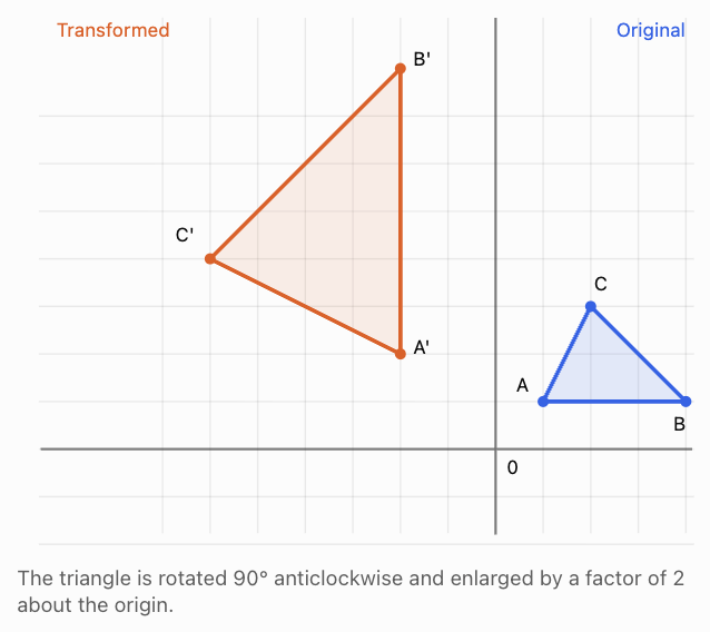
Step 6: Determine the effect on side lengths.
Multiplication by 2i has modulus 2.
Therefore, every side length is multiplied by 2.
The triangle remains similar to the original.
Step 7: Determine the effect on area.
An enlargement by scale factor 2 multiplies area by:
2² = 4
Therefore, the transformed triangle has four times the original area.
Step 8: Verify using side AB.
Original vertices:
A = (1, 1)
B = (4, 1)
Original length:
AB = √[(4 − 1)² + (1 − 1)²]
AB = 3
Transformed vertices:
A' = (−2, 2)
B' = (−2, 8)
Transformed length:
A'B' = √[(−2 + 2)² + (8 − 2)²]
A'B' = √36
A'B' = 6
Verification: 6/3 = 2
The side length has doubled, exactly as expected.
Final Challenge Summary
Property
Result
Transformation multiplier
2i
Rotation
90° anticlockwise
Enlargement factor
2
New vertex A
−2 + 2i
New vertex B
−2 + 8i
New vertex C
−6 + 4i
Side-length scale factor
2
Area scale factor
4
Conclusion
Complex numbers and trigonometry provide two complementary ways to understand mathematical relationships involving magnitude and direction.
Rectangular form describes complex numbers using real and imaginary components, while polar form expresses them using modulus and argument.
The connection to sine and cosine makes it possible to interpret complex numbers as points and vectors in a plane.
Polar form also transforms multiplication and division into operations involving magnitudes and angles. De Moivre's theorem extends this relationship to powers, while the root formulas reveal beautiful geometric patterns and symmetry.
Complex multiplication can represent rotations and enlargements, making these ideas especially useful in computer graphics, robotics, engineering, and signal processing.
The central idea is that complex numbers combine algebra and geometry: their magnitudes describe size, their arguments describe direction, and their operations describe transformations.
-
4. Trigonometry in Science and Engineering
Learning outcomes
- I can apply trigonometry to physics problems.
- I can apply trigonometry to engineering and architecture.
- I can interpret wave motion using trigonometric functions.
- I can analyse periodic motion mathematically.
- I can solve practical STEM applications.
Introduction
Trigonometry is one of the most important mathematical tools used in science, engineering, architecture, and technology.
Whenever a problem involves angles, distances, forces, rotations, waves, or repeating motion, trigonometry provides methods for describing and calculating relationships.
Engineers use trigonometry to design bridges, calculate forces in structures, and determine the correct angles for supporting beams. Architects use it to calculate roof slopes, building heights, and the dimensions of complex structures. Physicists use it to analyse projectile motion, forces on inclined planes, circular motion, and oscillations.
Trigonometric functions also describe many natural and technological phenomena, including sound waves, alternating electrical signals, vibrations, and periodic motion.
For example, a pendulum swings back and forth, a rotating wheel moves through a repeating cycle, and a vibrating string produces a wave. Although these situations appear different, many can be described using sine and cosine functions.
The central idea is that trigonometry connects geometry with physical quantities, allowing us to turn real-world situations into mathematical models.
In this lesson, we will explore how trigonometry is applied to physics, engineering, architecture, wave motion, periodic systems, and practical STEM problems.
The Mathematical Foundations
Before exploring applications, we need to understand several important trigonometric relationships.
Right-Triangle Trigonometry
For a right triangle with an acute angle θ:
sin θ = opposite / hypotenuse
cos θ = adjacent / hypotenuse
tan θ = opposite / adjacent
These relationships allow us to calculate unknown distances and angles.
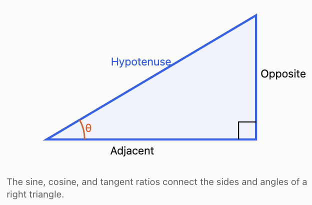
Resolving a Vector into Components
Many scientific quantities have both magnitude and direction.
These quantities are called vectors.
Examples include:
-
Force
-
Velocity
-
Acceleration
-
Displacement
-
Momentum
A vector of magnitude V making an angle θ above the positive horizontal axis has components:
Vₓ = V cos θ
Vᵧ = V sin θ
These formulas are fundamental in physics and engineering.
The Pythagorean Theorem
If perpendicular components are known:
V = √(Vₓ² + Vᵧ²)
The direction can be found from:
tan θ = Vᵧ/Vₓ
The correct quadrant must be considered when determining θ.
General Sinusoidal Model
Many repeating physical processes can be approximated by:
y(t) = A sin(ωt + φ) + D
or:
y(t) = A cos(ωt + φ) + D
where:
-
A is the signed amplitude coefficient.
-
|A| is the amplitude.
-
ω is the angular frequency.
-
φ is the phase constant.
-
D is the equilibrium or midline value.
-
t is time.
For ω ≠ 0:
Period: T = 2π/|ω|
Frequency: f = 1/T
Angular frequency: |ω| = 2πf
These relationships will appear repeatedly throughout the lesson.
Learning Target 1: Applying Trigonometry to Physics Problems
Forces Acting at Angles
Forces often act at angles rather than directly horizontally or vertically.
To analyse the motion of an object, we resolve each force into perpendicular components.
Suppose a force F acts at an angle θ above the horizontal.
Its components are:
Fₓ = F cos θ
Fᵧ = F sin θ
Worked Example 1: Pulling a Sled
A person pulls a sled with a force of 120 N at an angle of 30° above the horizontal.
Calculate the horizontal and vertical components of the force.
Step 1: Calculate the horizontal component.
Fₓ = 120 cos 30°
Fₓ = 120(√3/2)
Fₓ ≈ 103.9 N
Step 2: Calculate the vertical component.
Fᵧ = 120 sin 30°
Fᵧ = 120(0.5)
Fᵧ = 60 N
Interpretation: The horizontal component helps move the sled forward, while the upward component reduces the normal force exerted by the ground, provided the sled remains in contact with it.
Forces on an Inclined Plane
An inclined plane is a sloping surface.
When an object rests on a slope, gravity acts vertically downward.
The gravitational force can be resolved into two components:
-
Parallel to the slope.
-
Perpendicular to the slope.
For a slope angle θ:
F∥ = mg sin θ
F⊥ = mg cos θ
where m is mass and g is gravitational acceleration.
Worked Example 2: A Box on a Ramp
A 20 kg box rests on a frictionless ramp inclined at 25° to the horizontal.
Calculate:
a) The component of weight parallel to the ramp.
b) The component of weight perpendicular to the ramp.
c) The acceleration of the box if released.
Take g = 9.8 m/s².
Step 1: Calculate the weight.
W = mg
W = 20 × 9.8
W = 196 N
Step 2: Parallel component.
F∥ = 196 sin 25°
F∥ ≈ 82.8 N
Step 3: Perpendicular component.
F⊥ = 196 cos 25°
F⊥ ≈ 177.6 N
Step 4: Calculate acceleration.
On a frictionless ramp, the net force along the slope is mg sin θ.
Using Newton's Second Law:
ma = mg sin θ
Cancel m:
a = g sin θ
a = 9.8 sin 25°
a ≈ 4.14 m/s² down the slope
The mass cancels because gravitational acceleration along a frictionless slope does not depend on the object's mass.
Projectile Motion
When an object is launched at an angle, its initial velocity can be divided into horizontal and vertical components.
For initial speed v₀ and launch angle θ:
vₓ = v₀ cos θ
vᵧ = v₀ sin θ
Ignoring air resistance:
x(t) = v₀ cos θ × t
y(t) = y₀ + v₀ sin θ × t − ½gt²
where y₀ is the initial height.
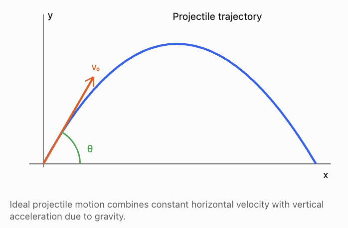
Worked Example 3: Launching a Ball
A ball is launched at 25 m/s at an angle of 40° above the horizontal from ground level.
Ignore air resistance.
Calculate the initial horizontal and vertical velocities, maximum height, time of flight, and horizontal range.
Step 1: Horizontal velocity.
vₓ = 25 cos 40°
vₓ ≈ 19.15 m/s
Step 2: Initial vertical velocity.
vᵧ = 25 sin 40°
vᵧ ≈ 16.07 m/s
Step 3: Maximum height.
At maximum height, vertical velocity is zero.
Using:
v² = u² + 2as
0 = vᵧ² − 2gH
Therefore:
H = vᵧ²/(2g)
H = (25 sin 40°)²/(19.6)
H ≈ 13.18 m
Step 4: Time of flight.
Because the ball lands at the same height from which it was launched:
T = 2vᵧ/g
T = 2(25 sin 40°)/9.8
T ≈ 3.28 s
Step 5: Horizontal range.
R = vₓT
R ≈ 19.15 × 3.2795
R ≈ 62.8 m
The range can also be calculated using:
R = v₀² sin(2θ)/g
This formula is valid for level-ground projectile motion without air resistance.
Circular Motion
An object moving around a circle has a continuously changing direction.
If a point moves around a circle of radius r with angular position θ:
x = r cos θ
y = r sin θ
If the angular speed is constant:
θ = ωt + φ
Therefore:
x(t) = r cos(ωt + φ)
y(t) = r sin(ωt + φ)
These equations connect circular motion directly to trigonometric functions.
For uniform circular motion:
v = r|ω|
a꜀ = v²/r = rω²
where a꜀ is the magnitude of centripetal acceleration, directed toward the centre.
Worked Example 4: Rotating Wheel
A wheel has a radius of 0.40 m and rotates at 3 revolutions per second.
Calculate its angular speed and the tangential speed of a point on its rim.
Frequency:
f = 3 Hz
Angular speed:
ω = 2πf
ω = 6π rad/s
ω ≈ 18.85 rad/s
Tangential speed:
v = rω
v = 0.40(6π)
v ≈ 7.54 m/s
This is the speed of a point on the rim, even though its velocity direction continually changes.
Learning Target 2: Applying Trigonometry to Engineering and Architecture
Trigonometry is essential when designing structures that must be safe, stable, and accurately constructed.
Engineers and architects regularly calculate heights, slopes, lengths, angles, and force components.
Roof Pitch and Building Design
The pitch of a roof describes its steepness.
For a roof inclined at angle θ to the horizontal:
tan θ = rise/run
where:
-
Rise is the vertical height gained.
-
Run is the horizontal distance.
-
θ is the roof angle.
The sloping length of a roof section can be calculated using:
L = run/cos θ
or:
L = rise/sin θ
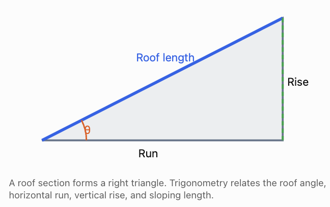
Worked Example 5: Designing a Roof
A symmetrical pitched roof covers a building 12 m wide. The roof rises at an angle of 35° from each outer wall toward the central ridge.
Calculate the height of the ridge above the walls and the sloping length of one roof section.
Step 1: Determine the run.
Because the roof is symmetrical:
Run = 12/2 = 6 m
Step 2: Calculate the rise.
tan 35° = rise/6
Rise = 6 tan 35°
Rise ≈ 4.20 m
Step 3: Calculate the sloping length.
cos 35° = 6/L
L = 6/cos 35°
L ≈ 7.32 m
Interpretation: Each sloping side is approximately 7.32 m long, and the ridge is approximately 4.20 m above the tops of the outer walls.
In a real roof design, engineers must also account for structural thickness, overhangs, loads, drainage, and building regulations.
Trigonometry in Structural Forces
A bridge or roof truss contains members arranged in triangular patterns.
Triangles are useful because their geometry provides rigidity when joints and members behave as designed.
Forces in inclined members can be resolved into horizontal and vertical components.
Consider two identical support cables making an angle θ above the horizontal and supporting a vertical load W.
If the system is symmetrical and in static equilibrium:
2T sin θ = W
Therefore:
T = W/(2 sin θ)
where T is the tension in each cable.
Worked Example 6: Supporting a Suspended Load
A 1000 N load is supported by two identical cables, each inclined at 40° above the horizontal.
Find the tension in each cable.
Vertical equilibrium requires:
2T sin 40° = 1000
T = 1000/(2 sin 40°)
T ≈ 778 N
The horizontal components of the two cable tensions cancel because the arrangement is symmetrical.
If the cables were closer to horizontal, the tension required in each cable would be greater.
This is an important engineering consideration.
Surveying and Measuring Inaccessible Heights
Surveyors use trigonometry to measure objects that cannot be measured directly.
For example, the height of a building can be determined from a horizontal distance and an angle of elevation.
If the observer's instrument is at height h₀:
Building height = d tan θ + h₀
where d is the horizontal distance to the building.
Worked Example 7: Measuring a Tower
A surveyor stands 80 m from a tower. The angle of elevation to the top is 38°. The survey instrument is 1.5 m above the ground.
Calculate the tower's height, assuming level ground.
Height above instrument:
h = 80 tan 38°
h ≈ 62.50 m
Add instrument height:
H = 62.50 + 1.5
Tower height ≈ 64.00 m
Surveying with Two Observation Points
Sometimes a direct distance cannot be measured, such as when surveying across a river.
The Law of Sines and Law of Cosines can be used with a measured baseline and observation angles.
Worked Example 8: Measuring Across a River
Two survey stations, A and B, are 150 m apart on the same side of a river.
A landmark C lies across the river.
The measured triangle angles are:
∠A = 48°
∠B = 67°
Calculate AC.
Step 1: Find angle C.
C = 180° − 48° − 67°
C = 65°
Step 2: Apply the Law of Sines.
AC/sin 67° = AB/sin 65°
AC = 150 sin 67°/sin 65°
AC ≈ 152.35 m
The distance from station A to the landmark is approximately 152 m.
This is an example of triangulation, where distances are determined from measured angles and a known baseline.
Structural Safety and Model Limitations
Trigonometry helps determine geometry and force components, but it does not by itself guarantee a safe structure.
Actual engineering design must also consider material strength, buckling, joint behaviour, wind, earthquakes, load combinations, and appropriate safety factors.
Learning Target 3: Interpreting Wave Motion Using Trigonometric Functions
Waves are disturbances that transfer energy through a medium or, in the case of electromagnetic waves, through fields.
Many waves can be approximated by sine or cosine functions.
Examples include:
-
Sound waves.
-
Water waves.
-
Light and other electromagnetic waves.
-
Vibrations in strings.
-
Alternating electrical signals.
The Sinusoidal Wave Model
A simple travelling wave can be represented by:
y(x, t) = A sin(kx − ωt + φ)
where:
-
y is the displacement from equilibrium.
-
A is amplitude.
-
x is position.
-
t is time.
-
k is angular wave number.
-
ω is angular frequency.
-
φ is the phase constant.
For a wave travelling in the positive x-direction, the form kx − ωt is commonly used.
Important Wave Quantities
Amplitude (A)
The maximum displacement from equilibrium.
Wavelength (λ)
The distance between consecutive points in the same phase, such as successive crests.
Period (T)
The time required for one complete oscillation.
Frequency (f)
The number of oscillations per second.
Wave speed (v)
The rate at which the wave pattern propagates.
The main relationships are:
f = 1/T
v = fλ
k = 2π/λ
ω = 2πf = 2π/T
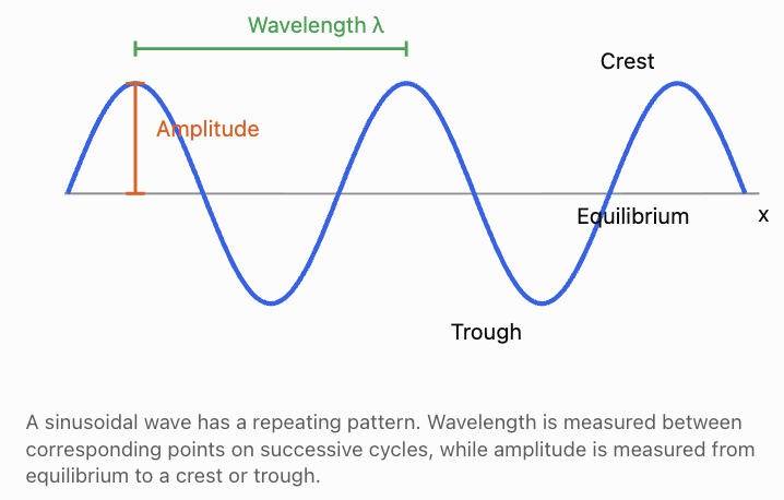
Worked Example 9: Calculating Wave Properties
A wave is described at a fixed instant by:
y(x) = 0.08 sin(4πx)
where x and y are measured in metres.
Find the amplitude and wavelength.
Step 1: Identify amplitude.
The coefficient of sine is 0.08.
Amplitude = 0.08 m
Step 2: Identify wave number.
k = 4π rad/m
Step 3: Calculate wavelength.
λ = 2π/k
λ = 2π/(4π)
Wavelength = 0.50 m
If the wave travels at 3 m/s, its frequency is:
f = v/λ
f = 3/0.50
Frequency = 6 Hz
Worked Example 10: A Travelling Wave
A wave is modelled by:
y(x, t) = 0.05 sin(2πx − 10πt)
where x and y are in metres and t is in seconds.
Find the amplitude, wavelength, frequency, period, and wave speed.
Step 1: Amplitude.
A = 0.05 m
Step 2: Wavelength.
k = 2π
λ = 2π/(2π)
λ = 1 m
Step 3: Frequency.
ω = 10π
f = ω/(2π)
f = 5 Hz
Step 4: Period.
T = 1/f
T = 0.20 s
Step 5: Wave speed.
v = fλ
v = 5 × 1
v = 5 m/s
The negative sign in kx − ωt indicates propagation in the positive x-direction when k and ω are positive.
Sound Waves
Sound is a mechanical wave that travels through a medium.
In air, sound is primarily a longitudinal pressure wave.
A simplified pressure variation at a fixed location can be modelled by:
Δp(t) = P sin(2πft + φ)
where P is pressure amplitude.
Frequency is closely related to perceived pitch, while pressure amplitude is related to sound intensity. Perceived loudness also depends on frequency and human hearing sensitivity.
Worked Example 11: Sound Frequency
A sound wave has a frequency of 440 Hz.
Calculate its period.
T = 1/f
T = 1/440
T ≈ 0.00227 s = 2.27 ms
The pressure pattern completes approximately 440 cycles each second.
Phase Difference
Two waves can have the same frequency and amplitude but reach their peaks at different times.
For example:
y₁(t) = 3 sin(2πt)
y₂(t) = 3 sin(2πt + π/2)
The second wave has a phase lead of π/2 radians, or 90°.
For waves with the same angular frequency, a phase difference Δφ corresponds to a time shift with magnitude:
|Δt| = |Δφ|/ω
Interference
When waves overlap, their displacements add according to the superposition principle in a linear medium.
If two equal-amplitude waves are in phase, they reinforce each other.
If they differ in phase by 180°, they cancel completely when their amplitudes are equal.
This is the basis of many technologies, including noise cancellation, interference measurement, and wave-based sensing.
Learning Target 4: Analysing Periodic Motion Mathematically
Periodic motion occurs when a system repeats its behaviour after a fixed time interval.
Examples include a vibrating spring, a rotating wheel, and an idealized pendulum.
Simple Harmonic Motion
Simple harmonic motion (SHM) occurs when the acceleration of an object is directly proportional to its displacement from equilibrium and acts in the opposite direction.
Mathematically:
a = −ω²x
A typical displacement model is:
x(t) = A cos(ωt + φ)
where A is the amplitude and φ determines the initial phase.
For ideal SHM:
v(t) = −Aω sin(ωt + φ)
a(t) = −Aω² cos(ωt + φ)
Therefore:
v(max) = Aω
a(max) = Aω²
Here v(max) and a(max) mean the maximum magnitudes of velocity and acceleration.
Worked Example 12: A Vibrating Spring
A mass attached to a spring oscillates according to:
x(t) = 0.12 cos(5πt)
where x is measured in metres and t in seconds.
Find the amplitude, angular frequency, frequency, period, maximum speed, and maximum acceleration.
Step 1: Amplitude.
A = 0.12 m
Step 2: Angular frequency.
ω = 5π rad/s
Step 3: Frequency.
f = ω/(2π)
f = 5π/(2π)
f = 2.5 Hz
Step 4: Period.
T = 1/f
T = 0.40 s
Step 5: Maximum speed.
v(max) = Aω
v(max) = 0.12(5π)
v(max) ≈ 1.88 m/s
Step 6: Maximum acceleration.
a(max) = Aω²
a(max) = 0.12(5π)²
a(max) ≈ 29.61 m/s²
Position, Velocity, and Acceleration
These quantities do not reach their maximum magnitudes at the same time.
For x(t) = A cos(ωt):
-
At maximum positive displacement, velocity is zero and acceleration is most negative.
-
At equilibrium, speed is greatest and acceleration is zero.
-
At maximum negative displacement, velocity is zero and acceleration is most positive.
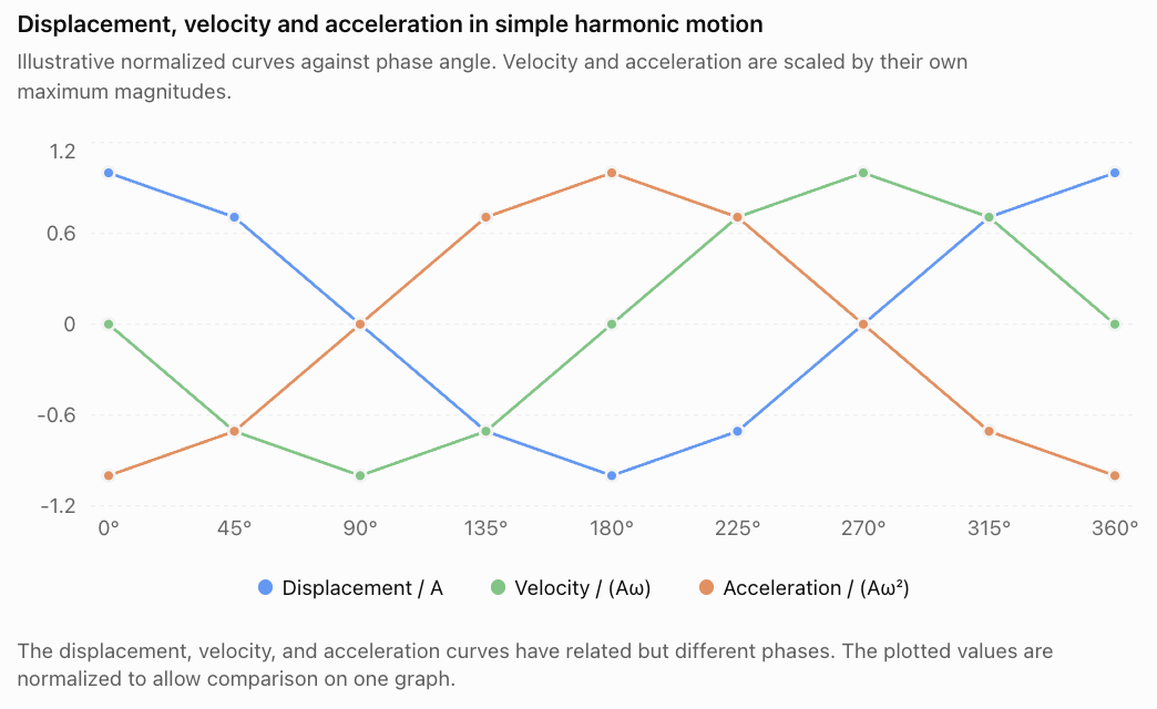
Pendulum Motion
For a simple pendulum of length L undergoing small oscillations:
T ≈ 2π√(L/g)
where g is gravitational acceleration.
This formula assumes a point mass, a massless string, negligible friction, and a sufficiently small swing angle.
Worked Example 13: Pendulum Period
A simple pendulum has a length of 1.5 m.
Calculate its approximate period using g = 9.8 m/s².
T = 2π√(1.5/9.8)
T ≈ 2.46 s
The pendulum completes one full oscillation approximately every 2.46 seconds.
For large swing angles, the period is longer than this small-angle approximation predicts.
Spring-Mass Systems
For an ideal mass attached to a spring obeying Hooke's law:
F = −kx
where k is the spring constant.
Newton's Second Law gives:
ma = −kx
Therefore:
a = −(k/m)x
Comparing this with a = −ω²x:
ω = √(k/m)
and:
T = 2π√(m/k)
Worked Example 14: Designing a Spring Oscillator
A mass of 0.50 kg is attached to a spring with spring constant 200 N/m.
Find the natural angular frequency and period.
Angular frequency:
ω = √(200/0.50)
ω = √400
ω = 20 rad/s
Period:
T = 2π/20
T ≈ 0.314 s
Damped Oscillations
Real systems lose energy due to friction, air resistance, or other dissipative effects.
Their amplitude often decreases over time.
A simplified underdamped model is:
x(t) = Ae^(−bt) cos(ωdt + φ)
where b > 0 is a decay constant and ωd is the damped angular frequency.
The exponential factor reduces the amplitude as time increases.
This type of model is useful for vehicle suspension, vibration control, and mechanical testing.
Resonance
Resonance occurs when a driven system responds strongly near one of its natural frequencies.
For example, a mechanical structure may vibrate significantly when exposed to periodic forcing near a natural frequency.
Engineers use trigonometric and differential-equation models to investigate resonance and reduce the risk of damaging vibrations.
Learning Target 5: Solving Practical STEM Applications
Many real-world problems combine several trigonometric ideas rather than using only one formula.
The key is to identify the physical quantities, construct a suitable model, and interpret the result.
Worked Example 15: Designing a Solar Panel
A solar panel has an area of 2.0 m².
Sunlight strikes the panel at an angle of 25° from the panel's normal (the direction perpendicular to its surface).
Calculate the effective projected area facing the incoming sunlight.
The projected area is:
A(effective) = A cos θ
Therefore:
A(effective) = 2.0 cos 25°
A(effective) ≈ 1.81 m²
This means the panel intercepts the same amount of direct radiation as a 1.81 m² surface oriented perpendicular to the rays, under the idealized geometric model.
Actual electrical output also depends on irradiance, panel efficiency, temperature, shading, and other factors.
Worked Example 16: A Wind Turbine Blade
A wind turbine blade is 30 m long and rotates at 15 revolutions per minute.
Calculate its angular speed and the tangential speed at its tip.
Step 1: Convert frequency to revolutions per second.
f = 15/60
f = 0.25 Hz
Step 2: Angular speed.
ω = 2πf
ω = 0.5π
ω ≈ 1.57 rad/s
Step 3: Tip speed.
v = rω
v = 30(0.5π)
v ≈ 47.12 m/s
The tip moves much faster than points closer to the centre because tangential speed is proportional to radius.
Worked Example 17: Aircraft Navigation
An aircraft travels at an airspeed of 200 km/h on a heading of 060°, measured clockwise from north.
Assume no wind.
Calculate its eastward and northward velocity components.
For a compass bearing β:
East component = v sin β
North component = v cos β
East:
v(E) = 200 sin 60°
v(E) ≈ 173.2 km/h
North:
v(N) = 200 cos 60°
v(N) = 100 km/h
This differs from the standard polar-angle convention because compass bearings are measured clockwise from north.
Worked Example 18: Analysing an Electrical Signal
An ideal alternating voltage is modelled by:
V(t) = 170 sin(100πt)
where V is in volts and t is in seconds.
Find the peak voltage, frequency, period, and root mean square (RMS) voltage.
Step 1: Peak voltage.
V(peak) = 170 V
Step 2: Angular frequency.
ω = 100π rad/s
Step 3: Frequency.
f = ω/(2π)
f = 50 Hz
Step 4: Period.
T = 1/f
T = 0.020 s
Step 5: RMS voltage.
For a pure sinusoidal voltage:
V(RMS) = V(peak)/√2
V(RMS) = 170/√2
V(RMS) ≈ 120.2 V
RMS voltage is useful because it relates an alternating voltage to its equivalent heating effect in a resistor.
Worked Example 19: Measuring a Bridge Support
An engineer observes the top of a vertical bridge support at an elevation angle of 28° from a point 45 m away horizontally.
The observation instrument is 1.7 m above the base level.
Find the support's height above that level.
Height above instrument:
h = 45 tan 28°
h ≈ 23.93 m
Total height:
H = 23.93 + 1.7
H ≈ 25.63 m
This result assumes the horizontal distance is measured accurately and the base and instrument reference levels are correctly established.
Choosing an Appropriate Trigonometric Method
Problem type
Useful method
Finding a height from distance and angle
Tangent
Finding components of a force
Sine and cosine
Calculating motion along a slope
Weight components
Analysing projectile motion
Velocity components and kinematics
Finding unknown sides in a non-right triangle
Law of Sines or Law of Cosines
Analysing wave frequency and wavelength
v = fλ
Modelling periodic displacement
Sine or cosine functions
Calculating rotation speed
ω = 2πf and v = rω
Analysing ideal spring oscillations
T = 2π√(m/k)
Analysing small-angle pendulum motion
T ≈ 2π√(L/g)
Calculating phase differences
Angular phase relationships
Analysing alternating electrical signals
Sinusoidal models and RMS relationships
The most important step is not memorizing every formula independently. It is recognizing the underlying geometry or repeating pattern.
A General Strategy for STEM Problems
Trigonometric applications become easier when we use a systematic approach.
Step 1: Understand the physical situation.
Identify what is happening and which quantities are known.
Step 2: Draw a diagram.
Include angles, lengths, directions, forces, or wave features.
Step 3: Identify the mathematical relationship.
Decide whether the problem requires triangle trigonometry, vector components, circular motion, or a sinusoidal model.
Step 4: Check units and angle conventions.
Distinguish degrees from radians, compass bearings from standard mathematical angles, and frequencies in hertz from angular frequencies in radians per second.
Step 5: Solve symbolically when possible.
Rearrange the formula before substituting numerical values.
Step 6: Calculate carefully.
Retain sufficient precision until the final answer.
Step 7: Interpret and verify.
Ask whether the result is physically reasonable and whether the model's assumptions are appropriate.
Common Mistakes
Mistake 1: Confusing Sine and Cosine When Resolving Forces
When θ is measured from the horizontal:
Fₓ = F cos θ
Fᵧ = F sin θ
If θ is measured from the vertical, the component relationships change accordingly.
Always use the angle shown in the diagram.
Mistake 2: Using the Wrong Angle Convention
Compass bearings are measured clockwise from north.
Standard mathematical angles are measured anticlockwise from the positive x-axis.
Mistake 3: Forgetting Units
Frequency is measured in hertz.
Angular frequency is measured in radians per second.
Wavelength is measured in metres.
Wave speed is measured in metres per second.
Mistake 4: Confusing Amplitude and Peak-to-Peak Value
If a vibration moves from −4 cm to +4 cm, its amplitude is 4 cm, not 8 cm.
Its peak-to-peak displacement is 8 cm.
Mistake 5: Confusing Frequency and Period
Frequency measures cycles per second.
Period measures seconds per cycle.
They are reciprocals:
f = 1/T
Mistake 6: Assuming All Motion Is Sinusoidal
Uniform circular motion has sinusoidal coordinate components, but not every type of periodic motion is simple harmonic.
Some periodic systems contain multiple frequencies, nonlinear effects, or changing amplitudes.
Mistake 7: Applying Projectile Formulas Outside Their Assumptions
The standard range formula R = v₀²sin(2θ)/g assumes that launch and landing heights are equal and air resistance is negligible.
Mistake 8: Assuming the Normal Force Always Equals mg
On an inclined plane without other perpendicular forces:
N = mg cos θ
It is not generally equal to mg.
Mistake 9: Ignoring Model Limitations
Real structures and machines may experience friction, drag, damping, deformation, turbulence, and other effects absent from simplified models.
Mistake 10: Reporting Unrealistic Precision
Measurements have limited precision.
A calculated building height of 64.003728 m is usually inappropriate if the input measurements are only accurate to a few centimetres or less.
Key Terms
-
Trigonometry: The study of relationships involving angles and lengths.
-
Vector: A quantity with magnitude and direction.
-
Scalar: A quantity with magnitude but no direction.
-
Component: The part of a vector acting along a chosen axis.
-
Resultant force: The vector sum of all forces acting on an object.
-
Inclined plane: A sloping surface.
-
Angle of elevation: The angle measured upward from the horizontal to an object.
-
Projectile motion: Motion under gravity after launch, often modelled without air resistance.
-
Circular motion: Motion along a circular path.
-
Angular speed: Rate of change of angular position.
-
Centripetal acceleration: Acceleration directed toward the centre of circular motion.
-
Triangulation: Determining locations or distances using measured angles and a known baseline.
-
Wave: A propagating disturbance that transfers energy.
-
Amplitude: Maximum displacement from equilibrium.
-
Wavelength: Distance between corresponding points of consecutive wave cycles.
-
Frequency: Number of cycles per second.
-
Period: Time required for one cycle.
-
Angular frequency: Rate of change of phase in radians per second.
-
Phase: Position within a repeating cycle.
-
Phase difference: Difference between the phases of two oscillations.
-
Interference: The combination of overlapping waves.
-
Simple harmonic motion: Motion in which acceleration is proportional to displacement and opposite in direction.
-
Equilibrium position: Position where the net restoring force is zero.
-
Damping: Reduction of oscillation amplitude through energy loss.
-
Resonance: Strong response of a driven system near a natural frequency.
-
Root mean square: A measure related to the mean square of a varying quantity.
-
Mathematical model: A mathematical representation of a physical system.
-
Assumption: A condition accepted when constructing or applying a model.
Key Takeaways
-
Trigonometry is used throughout physics, engineering, architecture, and technology.
-
Sine and cosine resolve vectors into perpendicular components.
-
Inclined-plane forces depend on the sine and cosine of the slope angle.
-
Projectile motion combines horizontal and vertical motion.
-
Trigonometry helps calculate structural dimensions, slopes, tensions, and inaccessible distances.
-
Sine and cosine functions describe many waves and oscillations.
-
Wave speed, frequency, and wavelength satisfy v = fλ.
-
Angular frequency and period are related by ω = 2π/T.
-
Ideal simple harmonic motion can be described by sinusoidal displacement functions.
-
Uniform circular motion and oscillations share important trigonometric relationships.
-
Real-world applications require attention to units, assumptions, and physical meaning.
-
A mathematically correct answer must also be interpreted in context.
Check Your Understanding
Part A: Physics Applications
Question 1
A force of 80 N acts at 35° above the horizontal.
Calculate its horizontal and vertical components.
Question 2
A 12 kg object rests on a frictionless slope inclined at 20°.
Calculate the force acting down the slope and the object's acceleration.
Use g = 9.8 m/s².
Question 3
A ball is launched at 30 m/s at 45° above the horizontal from ground level.
Calculate its maximum height and horizontal range, ignoring air resistance.
Part B: Engineering and Architecture
Question 4
A roof has a horizontal run of 5 m and an inclination of 30°.
Find its rise and sloping length.
Question 5
A 600 N load is supported by two identical cables inclined at 50° above the horizontal.
Find the tension in each cable.
Question 6
A surveyor stands 60 m from a building and measures an angle of elevation of 42°. The instrument is 1.6 m above ground level.
Find the building's height.
Part C: Wave Motion
Question 7
A wave has frequency 25 Hz and wavelength 0.80 m.
Calculate its speed and period.
Question 8
A travelling wave is described by:
y(x, t) = 0.04 sin(5πx − 20πt)
Find its amplitude, wavelength, frequency, period, and speed.
Part D: Periodic Motion
Question 9
A vibrating object has displacement:
x(t) = 0.08 cos(8πt)
Calculate its amplitude, frequency, period, maximum speed, and maximum acceleration.
Question 10
A simple pendulum has a length of 0.80 m.
Calculate its approximate period for small oscillations.
Part E: Integrated STEM Applications
Question 11
A rotating machine has a radius of 0.60 m and rotates at 120 revolutions per minute.
Find its angular speed and tangential speed at the rim.
Question 12
An alternating voltage is given by:
V(t) = 325 sin(100πt)
Find its peak voltage, frequency, period, and RMS voltage.
Check Your Understanding — Fully Worked Answers
Answer 1: Force Components
Given:
F = 80 N
θ = 35°
Horizontal component:
Fₓ = 80 cos 35°
Fₓ ≈ 65.5 N
Vertical component:
Fᵧ = 80 sin 35°
Fᵧ ≈ 45.9 N
Answer 2: Object on a Slope
Weight:
W = mg = 12 × 9.8 = 117.6 N
Force down slope:
F∥ = mg sin 20°
F∥ = 117.6 sin 20°
F∥ ≈ 40.2 N
Acceleration:
a = g sin 20°
a ≈ 3.35 m/s² down the slope
Answer 3: Projectile Motion
Initial vertical velocity:
vᵧ = 30 sin 45°
vᵧ ≈ 21.21 m/s
Maximum height:
H = vᵧ²/(2g)
H = (30 sin 45°)²/19.6
H ≈ 22.96 m
Horizontal range:
R = v₀² sin(2θ)/g
R = 30² sin 90°/9.8
R ≈ 91.84 m
Answer 4: Roof Design
Rise:
h = 5 tan 30°
h ≈ 2.89 m
Sloping length:
L = 5/cos 30°
L ≈ 5.77 m
Answer 5: Cable Tension
Vertical equilibrium:
2T sin 50° = 600
T = 600/(2 sin 50°)
T ≈ 391.6 N per cable
Answer 6: Building Height
Height above instrument:
h = 60 tan 42°
h ≈ 54.02 m
Add instrument height:
H = 54.02 + 1.6
H ≈ 55.62 m
Answer 7: Wave Speed and Period
Given:
f = 25 Hz
λ = 0.80 m
Wave speed:
v = fλ
v = 25 × 0.80
v = 20 m/s
Period:
T = 1/f
T = 1/25
T = 0.040 s
Answer 8: Travelling Wave
Given:
y(x, t) = 0.04 sin(5πx − 20πt)
Amplitude:
A = 0.04 m
Wave number:
k = 5π
Wavelength:
λ = 2π/(5π)
λ = 0.40 m
Angular frequency:
ω = 20π
Frequency:
f = 20π/(2π)
f = 10 Hz
Period:
T = 1/10
T = 0.10 s
Wave speed:
v = fλ
v = 10 × 0.40
v = 4 m/s
Answer 9: Vibrating Object
Given:
x(t) = 0.08 cos(8πt)
Amplitude:
A = 0.08 m
Angular frequency:
ω = 8π rad/s
Frequency:
f = 8π/(2π)
f = 4 Hz
Period:
T = 1/4
T = 0.25 s
Maximum speed:
v(max) = Aω
v(max) = 0.08(8π)
v(max) ≈ 2.01 m/s
Maximum acceleration:
a(max) = Aω²
a(max) = 0.08(8π)²
a(max) ≈ 50.53 m/s²
Answer 10: Pendulum
Given:
L = 0.80 m
g = 9.8 m/s²
T ≈ 2π√(L/g)
T ≈ 2π√(0.80/9.8)
T ≈ 1.80 s
Answer 11: Rotating Machine
Frequency:
f = 120/60 = 2 Hz
Angular speed:
ω = 2πf
ω = 4π
ω ≈ 12.57 rad/s
Tangential speed:
v = rω
v = 0.60(4π)
v ≈ 7.54 m/s
Answer 12: Alternating Voltage
Given:
V(t) = 325 sin(100πt)
Peak voltage:
V(peak) = 325 V
Angular frequency:
ω = 100π
Frequency:
f = 100π/(2π)
f = 50 Hz
Period:
T = 1/50
T = 0.020 s
RMS voltage:
V(RMS) = 325/√2
V(RMS) ≈ 229.8 V
Final Integrated Challenge: Designing a Vibration-Control System
An engineer is testing a machine that vibrates horizontally.
Its displacement is modelled by:
x(t) = 0.015 cos(12πt)
where x is measured in metres and t in seconds.
The machine is mounted on a spring system supporting a 25 kg mass.
Assume ideal simple harmonic motion.
Tasks
-
Determine the amplitude.
-
Calculate the frequency and period.
-
Calculate the maximum speed.
-
Calculate the maximum acceleration.
-
Determine the effective spring constant.
-
Calculate the maximum restoring force.
-
Explain two limitations of the model.
Fully Worked Solution
Step 1: Amplitude
A = 0.015 m
Amplitude = 15 mm
Step 2: Angular frequency
ω = 12π rad/s
Step 3: Frequency
f = ω/(2π)
f = 12π/(2π)
f = 6 Hz
Step 4: Period
T = 1/f
T ≈ 0.167 s
Step 5: Maximum speed
v(max) = Aω
v(max) = 0.015(12π)
v(max) ≈ 0.565 m/s
Step 6: Maximum acceleration
a(max) = Aω²
a(max) = 0.015(12π)²
a(max) ≈ 21.32 m/s²
Step 7: Effective spring constant
For ideal spring-mass motion:
ω² = k/m
Therefore:
k = mω²
k = 25(12π)²
k ≈ 35,531 N/m
Step 8: Maximum restoring force
F(max) = kA
F(max) ≈ 35,531 × 0.015
F(max) ≈ 533 N
We can verify using Newton's Second Law:
F(max) = ma(max)
F(max) ≈ 25 × 21.32
F(max) ≈ 533 N
The two approaches agree.
Step 9: Evaluate the model
The model assumes that the motion is perfectly sinusoidal and that the spring system behaves linearly.
In reality, damping may reduce the amplitude, and machine operation may introduce additional frequencies or changing forces.
A more realistic model may need to include damping and external driving forces.
Final Challenge Summary
Quantity
Result
Amplitude
0.015 m
Frequency
6 Hz
Period
0.167 s
Angular frequency
12π rad/s
Maximum speed
0.565 m/s
Maximum acceleration
21.32 m/s²
Effective spring constant
35,531 N/m
Maximum restoring force
533 N
Conclusion
Trigonometry provides a mathematical foundation for understanding many of the most important relationships in science and engineering.
In physics, it allows us to resolve forces, calculate projectile trajectories, analyse circular motion, and understand oscillations.
In engineering and architecture, it helps determine structural dimensions, support forces, roof slopes, and inaccessible distances.
In wave science, sine and cosine functions describe repeating disturbances, allowing us to calculate amplitude, wavelength, frequency, period, and phase.
Periodic-motion models extend these ideas to springs, pendulums, rotating machinery, and vibrating systems.
The most important skill is learning to recognize the mathematical structure of a real-world situation, choose an appropriate trigonometric relationship, and interpret the result using the physical context.
Trigonometry is more than a method for calculating angles and lengths. It is a language for describing motion, forces, waves, structures, and the mathematical patterns that appear throughout science and engineering.
-
5. Comprehensive Problem Solving
Learning outcomes
- I can combine multiple trigonometric concepts to solve complex problems.
- I can select appropriate mathematical techniques.
- I can justify each step in my reasoning.
- I can communicate complete mathematical solutions.
- I can connect concepts from throughout the course.
Introduction
Many mathematical problems cannot be solved using a single formula or technique. Real-world situations often involve several connected relationships, and solving them requires us to combine ideas from different areas of trigonometry.
For example, determining the height of a mountain may require angles of elevation, right-triangle trigonometry, and the Law of Sines. Designing a rotating mechanical system may require circular motion, trigonometric functions, and equations involving time. Analysing a navigation route may involve bearings, vector components, the Law of Cosines, and inverse trigonometric functions.
In these situations, success depends on more than knowing formulas. We must understand the problem, choose appropriate mathematical tools, connect different relationships, justify our reasoning, and evaluate whether the final answer makes sense.
This lesson brings together the major concepts studied throughout trigonometry, including:
-
Right-triangle trigonometry and inverse functions.
-
Angles in radians and degrees.
-
The unit circle and trigonometric identities.
-
Trigonometric equations and inequalities.
-
The Law of Sines and Law of Cosines.
-
Bearings, navigation, and surveying.
-
Trigonometric graphs and periodic modelling.
-
Polar coordinates and parametric equations.
-
Complex numbers in polar form.
-
Applications in physics, engineering, and mathematics.
The central goal is to develop a flexible approach to mathematical problem solving: identify the structure of a problem, select efficient techniques, connect the results, and communicate a complete, justified solution.
Learning Target 1: Combining Multiple Trigonometric Concepts
Why Complex Problems Require Multiple Techniques
A simple trigonometry question may ask us to calculate the height of a triangle using a known angle and side length.
A more complex question may require us to calculate an unknown angle first, use it to determine a distance, and then apply that distance in a second calculation.
The key is recognizing that a complicated problem can often be divided into smaller, manageable stages.
Consider a surveying problem in which two observation points are separated by a known distance. Angles are measured to a distant tower, and we want to calculate its height.
We might need to:
-
Use the Law of Sines to calculate a horizontal distance.
-
Use tangent to calculate the height above the observer.
-
Add the instrument height.
-
Check whether the result is physically reasonable.
Each stage uses a familiar concept, but the complete problem requires several concepts working together.
A General Problem-Solving Framework
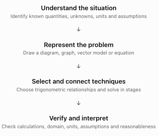
This framework is useful throughout mathematics, not only in trigonometry.
Learning Target 2: Selecting Appropriate Mathematical Techniques
A major part of advanced problem solving is deciding which technique is most appropriate.
Choosing a Technique
|
Problem characteristics |
Useful technique |
|---|---|
|
Right triangle with known sides or angles |
Sine, cosine, tangent |
|
Unknown angle from a trigonometric ratio |
Inverse trigonometric functions |
|
Non-right triangle with an angle and opposite side pair |
Law of Sines |
|
Non-right triangle with SAS or SSS information |
Law of Cosines |
|
Navigation using distances and directions |
Bearings and vector components |
|
Repeating behaviour over time |
Sine or cosine models |
|
Multiple solutions to a trigonometric equation |
Unit circle, identities, general solutions |
|
Rotations and positions around an origin |
Polar coordinates |
|
Motion described by time |
Parametric equations |
|
Complex-number powers and roots |
Polar form and De Moivre's theorem |
|
Forces at angles |
Vector resolution |
|
Maximum and minimum values |
Function analysis and trigonometric bounds |
Recognizing Hidden Triangles
Many problems do not explicitly mention a triangle.
For example:
-
A ladder leaning against a wall forms a right triangle.
-
Two forces acting at an angle form a vector triangle.
-
A navigation route with two successive journeys forms a triangle.
-
A support cable, vertical mast, and horizontal ground form a right triangle.
-
Two survey stations and a distant landmark form an oblique triangle.
Drawing an appropriate diagram often reveals the mathematics needed.
Worked Example 1: Choosing Between the Law of Sines and Law of Cosines
A triangle has sides of 12 cm and 17 cm with an included angle of 65°.
Find the third side.
Step 1: Identify the known information.
We know two sides and the angle between them.
This is a side-angle-side (SAS) situation.
Step 2: Select the appropriate technique.
The Law of Cosines is appropriate:
c² = a² + b² − 2ab cos C
Step 3: Substitute.
c² = 12² + 17² − 2(12)(17)cos 65°
c² = 144 + 289 − 408 cos 65°
c² ≈ 260.57
c ≈ √260.57
c ≈ 16.14 cm
Step 4: Verify.
The third side should be shorter than 12 + 17 = 29 cm and longer than |17 − 12| = 5 cm.
The result satisfies the triangle inequality.
It is also reasonable because the included angle is moderately large.
Worked Example 2: A Multi-Stage Surveying Problem
Two observation stations, A and B, are 200 m apart on level ground.
A tower stands at point C.
The measured horizontal angles are:
∠A = 52°
∠B = 73°
The angle of elevation from station A to the top of the tower is 18°.
Assume C is the base of the vertical tower and all three ground points are at the same elevation.
Find the tower's height.
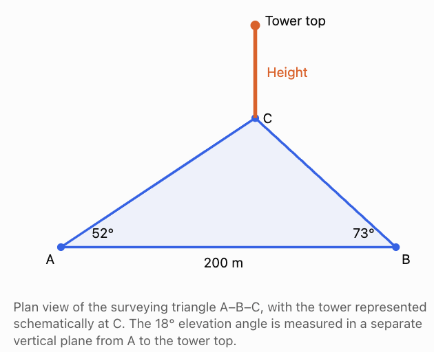
Step 1: Calculate angle C.
C = 180° − 52° − 73°
C = 55°
Step 2: Use the Law of Sines to find AC.
AC/sin 73° = 200/sin 55°
AC = 200 sin 73°/sin 55°
AC ≈ 233.48 m
Step 3: Use the angle of elevation.
Let h be the tower's height.
tan 18° = h/AC
h = AC tan 18°
h ≈ 233.48 tan 18°
h ≈ 75.86 m
Step 4: Interpret.
The tower is approximately 75.9 m tall.
The calculation combines an oblique-triangle relationship with right-triangle trigonometry.
Step 5: Evaluate assumptions.
The model assumes level ground, a vertical tower, accurate angle measurements, and a negligible instrument height. If the instrument is elevated, its height must be accounted for.
Learning Target 3: Justifying Mathematical Reasoning
A complete solution should explain not only what calculations were performed but also why they are valid.
What Makes a Mathematical Justification?
A strong justification identifies:
-
The mathematical principle being used.
-
Why the principle applies.
-
Any necessary assumptions.
-
The logical connection between steps.
-
The meaning of the result.
For example, instead of writing only:
x = 10 sin 35°
we can explain:
The vertical component of a 10-unit vector at 35° above the horizontal is found using sine because it is opposite the given angle.
The second explanation demonstrates mathematical understanding.
Worked Example 3: Proving a Trigonometric Identity
Prove:
(1 − cos² θ)/sin θ = sin θ
for sin θ ≠ 0.
Step 1: Identify the relevant identity.
The Pythagorean identity states:
sin² θ + cos² θ = 1
Therefore:
1 − cos² θ = sin² θ
Step 2: Substitute into the left-hand side.
(1 − cos² θ)/sin θ
= sin² θ/sin θ
Step 3: Simplify.
= sin θ
Therefore:
(1 − cos² θ)/sin θ = sin θ
for all θ where sin θ ≠ 0.
The identity is proven on its stated domain.
Why Domain Restrictions Matter
The original expression contains division by sin θ.
Therefore:
sin θ ≠ 0
This excludes:
θ = nπ
where n is any integer.
Even though the simplified expression sin θ is defined at those angles, the original expression is not.
A complete proof must preserve the original domain.
Worked Example 4: Solving an Equation with Full Justification
Solve:
2 sin² θ − 3 sin θ + 1 = 0
for 0° ≤ θ < 360°.
Step 1: Recognize the algebraic structure.
The equation is quadratic in sin θ.
Factor:
(2 sin θ − 1)(sin θ − 1) = 0
Step 2: Apply the zero-product property.
2 sin θ − 1 = 0
or:
sin θ − 1 = 0
Therefore:
sin θ = 1/2
or:
sin θ = 1
Step 3: Solve using the unit circle.
For sin θ = 1/2:
θ = 30°, 150°
For sin θ = 1:
θ = 90°
Step 4: State all solutions.
θ = 30°, 90°, 150°
Step 5: Verify.
At sin θ = 1/2:
2(1/4) − 3(1/2) + 1 = 0
At sin θ = 1:
2 − 3 + 1 = 0
All three angles satisfy the equation.
A Useful Communication Structure
For complex problems, organize your work using:
Given → Required → Method → Calculation → Verification → Interpretation
This helps make mathematical solutions clear, logical, and easy to follow.
Learning Target 4: Communicating Complete Mathematical Solutions
A mathematical solution should be understandable to someone who has not seen the problem before.
Good mathematical communication is especially important in engineering, science, research, and education because other people must be able to check the reasoning.
Writing a Complete Solution
A complete mathematical response should normally include:
-
A clear statement of the known information.
-
A definition of any variables.
-
A suitable diagram or mathematical model.
-
The formula or principle used.
-
Substitution and algebraic working.
-
A final answer with appropriate units.
-
Verification and interpretation.
Worked Example 5: Navigation and Resultant Displacement
A boat travels 18 km on a bearing of 040°, followed by 25 km on a bearing of 130°.
Find its resultant displacement and the bearing of its final position from its starting point.
Given:
First displacement = 18 km at 040°.
Second displacement = 25 km at 130°.
Required:
Resultant distance and bearing.
Method:
Resolve both displacements into eastward and northward components.
Because bearings are measured clockwise from north:
East component = d sin β
North component = d cos β
Step 1: First displacement.
E₁ = 18 sin 40° ≈ 11.57 km
N₁ = 18 cos 40° ≈ 13.79 km
Step 2: Second displacement.
E₂ = 25 sin 130° ≈ 19.15 km
N₂ = 25 cos 130° ≈ −16.07 km
The negative northward component indicates southward displacement.
Step 3: Add the components.
E = 11.57 + 19.15 ≈ 30.72 km
N = 13.79 − 16.07 ≈ −2.28 km
The final position is east and slightly south of the starting point.
Step 4: Calculate the resultant distance.
R = √(E² + N²)
Using unrounded components:
R ≈ 30.81 km
Step 5: Calculate the bearing.
The angle south of east is:
α = tan⁻¹(|N|/E)
α ≈ 4.25°
Because east corresponds to bearing 090°:
β = 90° + 4.25°
Bearing ≈ 094.25°
Step 6: Verify geometrically.
The two travel directions differ by 90°.
Therefore, the two displacement vectors are perpendicular.
Using Pythagoras:
R = √(18² + 25²)
R = √949
R ≈ 30.81 km
This agrees with the component method.
Final answer: The boat's resultant displacement is approximately 30.81 km on a bearing of 094.25°.
What Makes This a Strong Solution?
The solution explains the bearing convention, shows the component calculations, interprets the negative component, and verifies the magnitude using an independent method.
Learning Target 5: Connecting Concepts from Throughout Trigonometry
The most powerful applications arise when we recognize that different trigonometric topics describe related mathematical structures.
Connection 1: The Unit Circle and Trigonometric Functions
On the unit circle:
x = cos θ
y = sin θ
This explains why:
sin² θ + cos² θ = 1
It also connects trigonometry to coordinate geometry, periodic functions, polar coordinates, and complex numbers.
Connection 2: Circular Motion and Sinusoidal Motion
Consider a point moving around a circle of radius 5 with constant angular speed π/3 rad/s.
Its position can be modelled by:
x(t) = 5 cos(πt/3)
y(t) = 5 sin(πt/3)
The point moves around a circle, but each coordinate varies sinusoidally with time.
The period is:
T = 2π/(π/3)
T = 6 s
This means the point completes one revolution every 6 seconds.
Its horizontal and vertical coordinates also repeat every 6 seconds.
Worked Example 6: Connecting Parametric Equations and Trigonometric Graphs
A rotating wheel has radius 2 m. A point on its rim begins at the rightmost position and completes one revolution every 8 seconds.
Find parametric equations for its position, assuming anticlockwise rotation.
Step 1: Determine angular speed.
ω = 2π/T
ω = 2π/8
ω = π/4 rad/s
Step 2: Write the coordinate equations.
x(t) = 2 cos(πt/4)
y(t) = 2 sin(πt/4)
Step 3: Calculate the position after 2 seconds.
x(2) = 2 cos(π/2) = 0
y(2) = 2 sin(π/2) = 2
Position after 2 seconds: (0, 2)
Step 4: Interpret.
After 2 seconds, the wheel has completed one-quarter of a revolution.
The point has moved from the rightmost position to the top of the circle.
Connection 3: Polar Coordinates and Complex Numbers
A complex number in polar form is:
z = r(cos θ + i sin θ)
The same point in polar coordinates is:
(r, θ)
Therefore, polar coordinates and complex numbers use the same geometric quantities: magnitude and direction.
Worked Example 7: Rotation Using Complex Numbers
A point is represented by:
z = 3 + 4i
Rotate the point 60° anticlockwise about the origin.
Step 1: Determine the original modulus and argument.
r = √(3² + 4²) = 5
θ = tan⁻¹(4/3) ≈ 53.13°
Step 2: Add the rotation angle.
New argument:
θ(new) ≈ 53.13° + 60°
θ(new) ≈ 113.13°
Step 3: Write the new polar form.
z(new) = 5 cis 113.13°
Step 4: Convert to rectangular form.
Using the exact rotation multiplier:
z(new) = (3 + 4i)(cos 60° + i sin 60°)
= (3 + 4i)(1/2 + (√3/2)i)
Real part:
3/2 − 2√3
Imaginary part:
2 + 3√3/2
Therefore:
z(new) = (3/2 − 2√3) + (2 + 3√3/2)i
Approximately:
z(new) ≈ −1.964 + 4.598i
Step 5: Verify.
The modulus should remain 5 because rotation does not change distance from the origin.
√[(-1.964)² + 4.598²] ≈ 5
The result is consistent.
Connection 4: Trigonometric Identities and Wave Superposition
Suppose two oscillations have the same frequency:
y₁ = 3 sin t
y₂ = 4 cos t
Their combined displacement is:
y = 3 sin t + 4 cos t
This can be written as a single sinusoidal function:
y = R sin(t + φ)
Expanding:
R sin(t + φ) = R sin t cos φ + R cos t sin φ
Compare coefficients:
R cos φ = 3
R sin φ = 4
Square and add:
R²(cos² φ + sin² φ) = 9 + 16
R² = 25
R = 5
Also:
tan φ = 4/3
φ ≈ 53.13°
Therefore:
3 sin t + 4 cos t = 5 sin(t + 53.13°)
Here t and the phase angle must be interpreted in consistent units; equivalently, the expression is 5 sin(t + 0.9273) when t is in radians.
This technique is useful for combining oscillations of the same frequency.
Connection 5: The Law of Cosines and Vector Magnitudes
Suppose two vectors have magnitudes A and B and an angle θ between them.
Their resultant magnitude satisfies:
R² = A² + B² + 2AB cos θ
The plus sign appears because we are finding the magnitude of the vector sum.
This relationship can be derived from the Law of Cosines using the supplementary interior angle of the head-to-tail triangle.
Worked Example 8: Resultant Force
Two forces of 40 N and 60 N act on an object with an angle of 70° between them.
Find the magnitude of their resultant.
R² = 40² + 60² + 2(40)(60)cos 70°
R² = 1600 + 3600 + 4800 cos 70°
R² ≈ 6841.70
R ≈ 82.71 N
The result is between |60 − 40| = 20 N and 60 + 40 = 100 N, as expected.
Advanced Integrated Problem Solving
Worked Example 9: Combining a Trigonometric Model with an Inequality
The height of a seat on a Ferris wheel is modelled by:
h(t) = 18 − 15 cos(πt/20)
where h is measured in metres and t is measured in seconds.
The model begins with the seat at its lowest position.
Determine when the seat is at least 25 m above the ground during its first revolution.
Step 1: Determine the period.
ω = π/20
T = 2π/(π/20)
T = 40 s
Step 2: Form the inequality.
18 − 15 cos(πt/20) ≥ 25
Subtract 18:
−15 cos(πt/20) ≥ 7
Divide by −15, reversing the inequality:
cos(πt/20) ≤ −7/15
Step 3: Find the boundary angles.
Let:
u = πt/20
Then:
cos u = −7/15
For 0 ≤ u ≤ 2π, the boundary angles are approximately:
u₁ ≈ 2.056 rad
u₂ ≈ 4.227 rad
Cosine is at most −7/15 between these angles.
Step 4: Convert to time.
t = 20u/π
t₁ ≈ 13.09 s
t₂ ≈ 26.91 s
Final answer: The seat is at least 25 m above the ground from approximately 13.09 s to 26.91 s during the first revolution.
Verification: At t = 20 s, the seat is at its highest point:
h(20) = 18 − 15 cos π
h(20) = 33 m
Since 33 m is above 25 m, the interval correctly contains the highest point.
Worked Example 10: An Ambiguous Triangle Problem
A triangle has:
a = 12 cm
b = 16 cm
A = 40°
Determine all possible values of angle B and side c.
Step 1: Apply the Law of Sines.
sin B/b = sin A/a
sin B = 16 sin 40°/12
sin B ≈ 0.85705
Step 2: Determine possible angles.
B₁ ≈ 58.99°
B₂ = 180° − 58.99°
B₂ ≈ 121.01°
Step 3: Check both possibilities.
For B₁:
C₁ = 180° − 40° − 58.99°
C₁ ≈ 81.01°
For B₂:
C₂ = 180° − 40° − 121.01°
C₂ ≈ 18.99°
Both values are positive, so both triangles are possible.
Step 4: Find c in each triangle.
Using:
c/sin C = a/sin A
For the first triangle:
c₁ = 12 sin 81.01°/sin 40°
c₁ ≈ 18.44 cm
For the second triangle:
c₂ = 12 sin 18.99°/sin 40°
c₂ ≈ 6.07 cm
Final answer: Two triangles are possible, with approximately:
-
B = 58.99°, C = 81.01°, c = 18.44 cm.
-
B = 121.01°, C = 18.99°, c = 6.07 cm.
This demonstrates why the sine rule's ambiguous case must be checked rather than assuming the inverse sine gives the only answer.
Evaluating the Reasonableness of Solutions
A solution is not complete simply because a calculator produces a number.
We must determine whether the answer is mathematically and physically meaningful.
Check 1: Does the Answer Satisfy the Original Equation?
Substitute the result into the original equation whenever possible.
For trigonometric equations, this is particularly important after squaring, dividing, or using inverse functions.
Check 2: Is the Angle in the Correct Quadrant?
The signs of sine, cosine, and tangent depend on the quadrant.
For example, if a vector has a negative horizontal component and a positive vertical component, its direction must lie in Quadrant II.
Check 3: Are All Possible Solutions Included?
Trigonometric equations may have several solutions within a specified interval.
For example:
sin θ = 1/2
has two solutions between 0° and 360°:
θ = 30°, 150°.
Check 4: Does the Result Respect Physical Constraints?
A calculated distance cannot be negative.
An angle inside a triangle must be greater than 0° and less than 180°.
A triangle must satisfy the triangle inequality.
Check 5: Are the Units Correct?
A calculation involving speed and time should produce distance when the units are compatible.
A frequency should be expressed in hertz, not radians per second.
Check 6: Is the Model Appropriate?
A sinusoidal model may describe a repeating phenomenon well, but it may not account for irregular disturbances, damping, seasonal variation, or changing conditions.
A projectile model without air resistance may be useful for an introductory calculation but less accurate for a real object travelling at high speed.
Check 7: Is the Precision Reasonable?
A final answer should not imply more precision than the measurements support.
For example, if a distance is measured to the nearest metre, reporting a calculated height to six decimal places is usually misleading.
Common Mistakes
Mistake 1: Choosing a Formula Before Understanding the Problem
A familiar formula may not apply to the given information.
Better approach: Identify the geometry, known quantities, and unknowns before selecting a method.
Mistake 2: Assuming Every Triangle Is Right-Angled
The Pythagorean theorem and basic right-triangle ratios apply directly only to right triangles.
For non-right triangles, consider the Law of Sines or Law of Cosines.
Mistake 3: Ignoring the Ambiguous Case
The Law of Sines can produce two possible triangles in an SSA situation.
Check whether both possible angles produce valid triangles.
Mistake 4: Mixing Degrees and Radians
The period formula T = 2π/ω assumes angular quantities are expressed in radians.
Check calculator settings and the units used in the model.
Mistake 5: Confusing Bearings and Standard Angles
Bearings are measured clockwise from north.
Standard mathematical angles are measured anticlockwise from the positive x-axis.
Mistake 6: Using an Identity Without Considering Its Domain
Dividing by sin θ removes cases where sin θ = 0.
Such cases may contain valid solutions to the original equation and must be checked before division.
Mistake 7: Rounding Too Early
Rounding intermediate values can introduce noticeable errors in multi-stage problems.
Keep additional digits until the final calculation.
Mistake 8: Giving an Answer Without Justification
A numerical answer does not show why the selected method is valid.
State the relevant formula and explain its use.
Mistake 9: Failing to Interpret the Result
An answer of 120° might represent an interior triangle angle, a compass bearing, a phase difference, or a rotation.
Its meaning must be clear.
Mistake 10: Forgetting to Check Reasonableness
A negative physical distance, an impossible triangle, or a frequency with incorrect units should signal a need to review the calculation.
Key Terms
-
Comprehensive problem solving: Combining multiple mathematical ideas to solve a problem.
-
Mathematical reasoning: Using logical steps and mathematical principles to justify a conclusion.
-
Mathematical model: A representation of a real or abstract situation using mathematical relationships.
-
Assumption: A condition accepted when constructing a model or solution.
-
Verification: Checking whether a result satisfies the original conditions.
-
Reasonableness: Whether a result is consistent with mathematical and real-world constraints.
-
Right-triangle trigonometry: Relationships involving sine, cosine, and tangent in right triangles.
-
Inverse trigonometric function: A function used to determine an angle from a trigonometric value.
-
Unit circle: A circle of radius 1 centred at the origin.
-
Trigonometric identity: An equality involving trigonometric expressions that is valid throughout its stated domain.
-
Trigonometric equation: An equation containing trigonometric functions.
-
Law of Sines: A relationship between triangle sides and the sines of their opposite angles.
-
Law of Cosines: A relationship involving three sides and an included angle of a triangle.
-
Ambiguous case: An SSA triangle situation in which more than one triangle may satisfy the given information.
-
Bearing: A direction measured clockwise from north.
-
Vector component: The part of a vector acting along a chosen axis.
-
Resultant vector: The vector sum of two or more vectors.
-
Amplitude: Maximum displacement from the midline of a sinusoidal model.
-
Period: Length of one complete cycle.
-
Frequency: Number of cycles per unit time.
-
Phase shift: Horizontal displacement of a periodic graph.
-
Polar coordinates: Coordinates describing a point using radius and angle.
-
Parametric equations: Equations expressing coordinates using a common parameter.
-
Complex number: A number of the form a + bi.
-
Modulus: Magnitude of a complex number or vector.
-
Argument: Direction angle of a nonzero complex number.
-
De Moivre's theorem: A rule for powers of complex numbers in polar form.
-
Domain restriction: A limitation on values for which an expression or equation is defined.
-
Extraneous solution: A value introduced during algebraic manipulation that does not satisfy the original equation.
Key Takeaways
-
Complex problems often require several connected mathematical techniques.
-
Understanding the situation is more important than immediately selecting a formula.
-
Diagrams help reveal hidden geometric relationships.
-
Right-triangle trigonometry, the Law of Sines, and the Law of Cosines solve different triangle situations.
-
Trigonometric identities can simplify expressions and equations.
-
Trigonometric equations may have multiple solutions.
-
Vector components connect trigonometry with navigation, forces, and motion.
-
Sinusoidal models describe many repeating phenomena.
-
Polar coordinates, parametric equations, and complex numbers connect geometry with rotation.
-
Complete solutions should include explanations, calculations, units, verification, and interpretation.
-
The most effective technique is the one that matches the structure of the problem.
-
Mathematical results should always be checked for validity and reasonableness.
Check Your Understanding
These questions combine concepts from across the trigonometry course. Try to identify the appropriate techniques before beginning each calculation.
Part A: Triangles and Geometry
Question 1
A triangle has sides of 9 cm and 14 cm with an included angle of 75°.
Calculate the third side.
Question 2
A surveyor stands 50 m from a building on level ground and measures an angle of elevation of 32° to the top. The instrument is 1.6 m above the ground.
Calculate the building's height.
Question 3
A triangle has A = 35°, a = 10 cm, and b = 14 cm.
Determine whether one or two triangles are possible and calculate the possible values of angle B.
Part B: Trigonometric Identities and Equations
Question 4
Prove:
(1 − sin² θ)/cos θ = cos θ
State any necessary domain restrictions.
Question 5
Solve:
2 cos² θ − cos θ − 1 = 0
for 0° ≤ θ < 360°.
Part C: Navigation and Vectors
Question 6
A hiker walks 12 km east and then 9 km north.
Find the resultant displacement and its three-figure bearing.
Question 7
Two forces of 50 N and 70 N act at an angle of 60° to each other.
Find the magnitude of their resultant.
Part D: Periodic Models
Question 8
A rotating wheel has radius 3 m and completes one revolution every 12 seconds.
Write parametric equations for a point beginning at the rightmost position and rotating anticlockwise.
Find its position after 3 seconds.
Question 9
The height of a platform is modelled by:
h(t) = 12 + 5 sin(πt/6)
Find the midline, amplitude, period, maximum height, and minimum height.
Part E: Polar Coordinates and Complex Numbers
Question 10
Convert:
z = −3 + 3i
into polar form using a principal argument.
Question 11
Calculate:
(3 cis 40°)(4 cis 80°)
Give your answer in polar form.
Question 12
A point is represented by z = 2 + 3i.
It is rotated 90° anticlockwise about the origin and enlarged by a factor of 2.
Find its new position.
Check Your Understanding — Fully Worked Answers
Answer 1: Law of Cosines
Given:
a = 9 cm
b = 14 cm
C = 75°
Because two sides and the included angle are known, use the Law of Cosines.
c² = a² + b² − 2ab cos C
c² = 9² + 14² − 2(9)(14)cos 75°
c² = 81 + 196 − 252 cos 75°
c² ≈ 211.78
c ≈ 14.55 cm
Verification: 5 < 14.55 < 23, so the triangle inequality is satisfied.
Answer 2: Building Height
Given:
Horizontal distance = 50 m
Angle of elevation = 32°
Instrument height = 1.6 m
Let h be the height above the instrument.
tan 32° = h/50
h = 50 tan 32°
h ≈ 31.24 m
Add the instrument height:
H = 31.24 + 1.6
Building height ≈ 32.84 m
Answer 3: Ambiguous Case
Given:
A = 35°
a = 10 cm
b = 14 cm
Using the Law of Sines:
sin B/b = sin A/a
sin B = 14 sin 35°/10
sin B ≈ 0.8030
First possible angle:
B₁ ≈ 53.42°
Second possible angle:
B₂ = 180° − 53.42°
B₂ ≈ 126.58°
Check the triangle angle sums:
For B₁:
C₁ = 180° − 35° − 53.42° ≈ 91.58°
For B₂:
C₂ = 180° − 35° − 126.58° ≈ 18.42°
Both third angles are positive.
Two triangles are possible, with B ≈ 53.42° or B ≈ 126.58°.
Answer 4: Identity Proof
Prove:
(1 − sin² θ)/cos θ = cos θ
Start with the Pythagorean identity:
sin² θ + cos² θ = 1
Rearrange:
1 − sin² θ = cos² θ
Substitute:
(1 − sin² θ)/cos θ
= cos² θ/cos θ
= cos θ
Therefore, the identity is proven.
Domain restriction: cos θ ≠ 0.
This excludes θ = 90° + 180°n, where n is any integer.
Answer 5: Trigonometric Equation
Solve:
2 cos² θ − cos θ − 1 = 0
Factor:
(2 cos θ + 1)(cos θ − 1) = 0
Therefore:
cos θ = −1/2
or:
cos θ = 1
For cos θ = −1/2:
θ = 120°, 240°
For cos θ = 1:
θ = 0° within the given interval.
Solutions: θ = 0°, 120°, 240°
Answer 6: Navigation
The hiker travels:
East = 12 km
North = 9 km
Resultant distance:
R = √(12² + 9²)
R = √225
R = 15 km
Bearing is measured clockwise from north.
tan β = 12/9
β = tan⁻¹(12/9)
β ≈ 53.13°
Bearing ≈ 053°
Final answer: 15 km on a bearing of 053°, rounded to the nearest degree.
Answer 7: Resultant Force
Given:
F₁ = 50 N
F₂ = 70 N
Angle between forces = 60°
For the vector sum:
R² = F₁² + F₂² + 2F₁F₂ cos 60°
R² = 50² + 70² + 2(50)(70)(0.5)
R² = 2500 + 4900 + 3500
R² = 10,900
R ≈ 104.40 N
The result is reasonable because it lies between 20 N and 120 N.
Answer 8: Parametric Equations
Given:
Radius = 3 m
Period = 12 s
Angular speed:
ω = 2π/12 = π/6 rad/s
Since the point begins at the rightmost position and rotates anticlockwise:
x(t) = 3 cos(πt/6)
y(t) = 3 sin(πt/6)
At t = 3:
x(3) = 3 cos(π/2) = 0
y(3) = 3 sin(π/2) = 3
Position after 3 seconds: (0, 3)
This is one-quarter of a revolution.
Answer 9: Sinusoidal Model
Given:
h(t) = 12 + 5 sin(πt/6)
Midline:
h = 12
Amplitude:
A = 5
Angular frequency:
ω = π/6
Period:
T = 2π/(π/6)
T = 12 time units
Maximum height:
12 + 5 = 17
Minimum height:
12 − 5 = 7
Maximum height = 17 units
Minimum height = 7 units
The units depend on those assigned to h and t in the physical model.
Answer 10: Complex Number in Polar Form
Given:
z = −3 + 3i
Modulus:
r = √[(-3)² + 3²]
r = √18
r = 3√2
The point is in Quadrant II.
Reference angle:
α = tan⁻¹(3/3) = 45°
Principal argument:
θ = 180° − 45°
θ = 135°
z = 3√2 cis 135°
Answer 11: Complex Multiplication
Given:
z₁ = 3 cis 40°
z₂ = 4 cis 80°
Multiply moduli:
3 × 4 = 12
Add arguments:
40° + 80° = 120°
Answer: 12 cis 120°
Answer 12: Rotation and Enlargement
Given:
z = 2 + 3i
A 90° anticlockwise rotation corresponds to multiplication by i.
An enlargement by factor 2 corresponds to multiplication by 2.
Combined multiplier:
2i
Calculate:
z(new) = (2 + 3i)(2i)
z(new) = 4i + 6i²
Since i² = −1:
z(new) = 4i − 6
New complex number: −6 + 4i
New Cartesian position: (−6, 4)
Verification:
Original modulus = √(2² + 3²) = √13
New modulus = √[(-6)² + 4²] = √52 = 2√13
The distance from the origin has doubled, as expected.
Final Integrated Challenge: Designing a Rotating Observation System
An engineering team is designing a rotating observation platform.
A sensor is attached 8 m from the centre of rotation. The platform completes one anticlockwise revolution every 20 seconds.
At t = 0, the sensor is at the rightmost point of its circular path.
A stationary observation point P is located 12 m east and 5 m north of the centre.
The engineers need to determine the sensor's position, its distance from P, and the times when the sensor is directly north of the centre.
Tasks
-
Calculate the angular speed.
-
Write parametric equations for the sensor's position.
-
Find its position after 5 seconds.
-
Calculate the distance from the sensor to P after 5 seconds.
-
Find the times during the first revolution when the sensor is directly north of the centre.
-
Express the sensor's position after 5 seconds as a complex number.
-
Explain how the problem connects trigonometric functions, coordinate geometry, circular motion, and complex numbers.
Fully Worked Solution
Step 1: Angular speed
The platform completes one revolution every 20 seconds.
ω = 2π/T
ω = 2π/20
ω = π/10 rad/s
Step 2: Parametric equations
Radius = 8 m
The sensor begins at the rightmost position.
Therefore:
x(t) = 8 cos(πt/10)
y(t) = 8 sin(πt/10)
for 0 ≤ t ≤ 20.
Step 3: Position after 5 seconds
x(5) = 8 cos(π/2) = 0
y(5) = 8 sin(π/2) = 8
Sensor position: (0, 8)
Step 4: Distance to observation point P
P = (12, 5)
Sensor = (0, 8)
Use the distance formula:
d = √[(12 − 0)² + (5 − 8)²]
d = √(144 + 9)
d = √153 ≈ 12.37 m
Step 5: When is the sensor directly north?
The sensor is directly north of the centre when:
x = 0
and:
y > 0
Therefore:
cos(πt/10) = 0
with positive sine.
During the first revolution, this occurs at:
πt/10 = π/2
t = 5
The sensor is directly north after 5 seconds.
It is directly south after 15 seconds, which does not satisfy the condition.
Step 6: Complex-number representation
The sensor's position after 5 seconds is:
(0, 8)
Therefore:
z = 8i
In polar form:
z = 8 cis 90°
Step 7: Explain the connections
The problem uses several mathematical ideas:
-
Circular motion: Angular speed determines how quickly the sensor rotates.
-
Trigonometric functions: Sine and cosine determine horizontal and vertical coordinates.
-
Parametric equations: The position is expressed as a function of time.
-
Coordinate geometry: The distance formula determines the separation between two points.
-
Trigonometric equations: Solving cos θ = 0 identifies particular positions.
-
Complex numbers: The sensor's position can be represented using modulus and argument.
Final Challenge Summary
|
Quantity |
Result |
|---|---|
|
Radius |
8 m |
|
Period |
20 s |
|
Angular speed |
π/10 rad/s |
|
Horizontal position |
x(t) = 8 cos(πt/10) |
|
Vertical position |
y(t) = 8 sin(πt/10) |
|
Position after 5 s |
(0, 8) |
|
Distance to P after 5 s |
√153 ≈ 12.37 m |
|
Time directly north |
5 s |
|
Complex position after 5 s |
8i |
|
Polar complex form |
8 cis 90° |
Conclusion
Comprehensive trigonometric problem solving requires more than the ability to apply individual formulas.
It requires us to recognize relationships, select appropriate methods, organize calculations, justify reasoning, and connect mathematical results to the situation being studied.
Right-triangle trigonometry helps solve problems involving lengths and angles. The Law of Sines and Law of Cosines extend these methods to non-right triangles. Trigonometric identities and equations provide algebraic tools for simplifying and solving relationships. Periodic functions describe waves, oscillations, and repeating motion. Polar coordinates, parametric equations, and complex numbers provide additional ways to describe position, direction, and rotation.
These ideas are not separate mathematical topics. They are different parts of a connected system.
The ultimate goal of trigonometry is not simply to calculate unknown values, but to develop the ability to represent complex situations mathematically, reason through them logically, and communicate solutions that are accurate, complete, and meaningful.