Applications and Function Analysis
4. Real-World Modelling
Learning outcomes
- I can select appropriate polynomial or rational models.
- I can create mathematical models from data.
- I can evaluate the accuracy of models.
- I can interpret model parameters.
- I can solve real-world problems using function models.
Introduction
Mathematics is one of the most powerful tools we have for understanding the world. From predicting the height of a projectile to estimating business costs, analysing population changes, and planning transportation, mathematical functions allow us to describe relationships and make predictions.
However, real-world situations rarely come with an equation already provided. Instead, we must examine information, identify patterns, choose suitable mathematical functions, and evaluate whether our models accurately represent reality.
This process is called mathematical modelling.
Two important families of functions used in mathematical modelling are polynomial functions and rational functions.
Polynomial functions are particularly useful for describing relationships involving area, volume, motion, and changing trends. Rational functions are useful when one quantity depends on another through division, such as average cost, travel time, concentration, and work rates.
Choosing a suitable model requires more than finding an equation that fits a set of data. We must also understand the meaning of the variables, interpret the parameters, evaluate the accuracy of predictions, and recognize the limitations of the model.
In this lesson, we will develop a complete modelling process, beginning with real-world data and ending with mathematical predictions and conclusions.
What Is Mathematical Modelling?
A mathematical model is a mathematical representation of a real-world situation.
A model may take the form of:
-
An equation or function.
-
A table of values.
-
A graph.
-
A system of equations.
-
A mathematical relationship involving several variables.
For example, suppose a taxi company charges a fixed booking fee of $4 and an additional $2.50 per kilometre.
The total cost can be modelled by:
C(d) = 4 + 2.5d
where:
-
C(d) is the total cost in dollars.
-
d is the distance travelled in kilometres.
-
4 represents the fixed booking fee.
-
2.5 represents the cost per kilometre.
This is a linear polynomial model.
The model can be used to calculate the cost of a journey, compare transport options, or determine how far someone can travel with a fixed budget.
The Mathematical Modelling Cycle
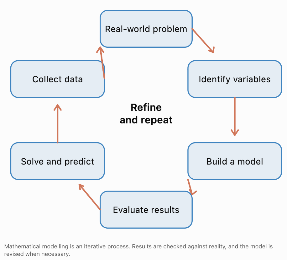
The modelling process generally involves six stages.
-
Understand the problem: Identify what needs to be calculated, explained, or predicted.
-
Define variables and assumptions: Decide which quantities matter and which simplifying assumptions are reasonable.
-
Collect and organize data: Use measurements, observations, tables, or other reliable information.
-
Choose and construct a model: Select an appropriate function and determine its parameters.
-
Use the model: Calculate values, solve equations, or make predictions.
-
Evaluate and refine: Compare predictions with observations and determine whether the model is suitable.
A model is useful when it captures the important features of a situation, even if it does not represent every detail perfectly.
Choosing Between Polynomial and Rational Models
Different mathematical relationships require different types of functions.
Polynomial Models
A polynomial function has the general form:
f(x) = aₙxⁿ + aₙ₋₁xⁿ⁻¹ + ... + a₁x + a₀
where the exponents are nonnegative integers.
Common examples include:
Linear: f(x) = mx + b
Quadratic: f(x) = ax² + bx + c
Cubic: f(x) = ax³ + bx² + cx + d
Polynomial models are often appropriate when:
-
A quantity changes at a constant rate.
-
A quantity changes at a constant second-difference rate for equally spaced inputs.
-
An area or volume depends on dimensions.
-
Motion is described using constant acceleration.
-
A smooth trend can be approximated over a limited interval.
Rational Models
A rational function has the form:
where P(x) and Q(x) are polynomials and Q(x) is not identically zero.
Rational models are often appropriate when:
-
One quantity is divided by another.
-
A relationship involves inverse variation.
-
A quantity approaches a limiting value.
-
Average cost depends on production quantity.
-
Travel time depends on speed.
-
Work rates or concentrations are involved.
Comparing Model Types
|
Situation |
Suitable model |
Reason |
|---|---|---|
|
Taxi fare with fixed fee |
Linear polynomial |
Constant cost per kilometre |
|
Projectile height |
Quadratic polynomial |
Constant acceleration |
|
Area of a square |
Quadratic polynomial |
Area depends on squared length |
|
Volume of a cube |
Cubic polynomial |
Volume depends on cubed length |
|
Travel time at varying speed |
Rational |
Time = distance/speed |
|
Average production cost |
Rational |
Total cost divided by quantity |
|
Inverse-square relationship |
Rational |
Output proportional to 1/x² |
|
Short-term curved trend |
Possibly polynomial |
Polynomial regression may approximate the data |
Important: A mathematical model should be chosen based on the relationship and the evidence, not merely because its graph resembles the data.
Identifying Patterns in Data
Before choosing a model, we should examine how the output changes as the input changes.
Constant First Differences
Consider:
|
x |
y |
|---|---|
|
0 |
3 |
|
1 |
7 |
|
2 |
11 |
|
3 |
15 |
|
4 |
19 |
The first differences are:
7 − 3 = 4
11 − 7 = 4
15 − 11 = 4
19 − 15 = 4
The first differences are constant.
This suggests a linear model:
y = 4x + 3
Constant Second Differences
Consider:
|
x |
y |
First difference |
Second difference |
|---|---|---|---|
|
0 |
2 |
— |
— |
|
1 |
5 |
3 |
— |
|
2 |
10 |
5 |
2 |
|
3 |
17 |
7 |
2 |
|
4 |
26 |
9 |
2 |
The first differences are 3, 5, 7, 9.
The second differences are constant at 2.
This suggests a quadratic model.
In fact:
y = x² + 2x + 2
Recognizing Inverse Relationships
Consider:
|
x |
y |
|---|---|
|
1 |
24 |
|
2 |
12 |
|
3 |
8 |
|
4 |
6 |
|
6 |
4 |
The product xy is constant:
1 × 24 = 24
2 × 12 = 24
3 × 8 = 24
This suggests:
y = 24/x
which is a rational model.
Recognizing a Limiting Value
Consider:
|
x |
y |
|---|---|
|
1 |
30 |
|
2 |
20 |
|
4 |
15 |
|
5 |
14 |
|
10 |
12 |
The values decrease toward 10.
This suggests a model of the form:
y = a/x + 10
Using x = 1, y = 30:
30 = a + 10
a = 20
Therefore:
y = 20/x + 10
The horizontal asymptote y = 10 represents the limiting value.
A Caution About Patterns
Constant differences identify polynomial degree only under suitable conditions, including equally spaced x-values and exact data generated by a polynomial.
Real measurements contain uncertainty and noise, so differences are rarely perfectly constant. In practice, graphs, regression, residuals, and scientific understanding should be considered together.
Creating Mathematical Models from Data
Once we identify a pattern, the next step is to construct an equation.
This may involve solving for unknown coefficients, using a regression tool, or applying a known scientific relationship.
Worked Example 1: Building a Linear Model
A delivery company records the following costs:
|
Distance (km) |
Cost ($) |
|---|---|
|
2 |
11 |
|
4 |
17 |
|
6 |
23 |
|
8 |
29 |
Find a model for delivery cost.
Step 1: Identify the relationship.
The cost increases by $6 whenever distance increases by 2 km.
Therefore, the rate of change is:
m = 6/2 = 3 dollars per kilometre.
Step 2: Use linear form.
C(d) = md + b
Substitute m = 3:
C(d) = 3d + b
Step 3: Find the fixed cost.
Using (2, 11):
11 = 3(2) + b
b = 5
Final model:
C(d) = 3d + 5
Step 4: Interpret the parameters.
-
3 represents the cost per kilometre.
-
5 represents the fixed delivery fee.
Step 5: Make a prediction.
For 12 km:
C(12) = 3(12) + 5 = 41
Predicted delivery cost: $41.
This prediction assumes the same pricing rule applies at 12 km.
Worked Example 2: Building a Quadratic Model
A student measures the height of a ball at different times.
|
Time (s) |
Height (m) |
|---|---|
|
0 |
2 |
|
1 |
17 |
|
2 |
22 |
|
3 |
17 |
|
4 |
2 |
We expect a quadratic model because the ball rises and then falls under approximately constant gravitational acceleration.
Use:
h(t) = at² + bt + c
Step 1: Find c.
At t = 0, h = 2.
Therefore:
c = 2
So:
h(t) = at² + bt + 2
Step 2: Use the point (1, 17).
17 = a + b + 2
a + b = 15
Step 3: Use the point (2, 22).
22 = 4a + 2b + 2
4a + 2b = 20
Divide by 2:
2a + b = 10
Step 4: Solve simultaneously.
2a + b = 10
a + b = 15
Subtract:
a = −5
Then:
−5 + b = 15
b = 20
Final model:
h(t) = −5t² + 20t + 2
Step 5: Verify the model.
At t = 3:
h(3) = −5(9) + 20(3) + 2
= −45 + 60 + 2
= 17
This matches the recorded height.
At t = 4:
h(4) = −80 + 80 + 2 = 2
Again, the model matches the data.
Visualizing the Model
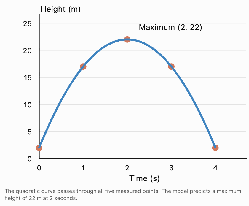
Interpretation of parameters:
-
a = −5 determines the downward curvature. In the ideal constant-acceleration model, a = −g/2.
-
b = 20 represents the initial vertical velocity in m/s.
-
c = 2 represents the initial height in metres.
The model is physically meaningful from launch until the ball reaches the ground, approximately 4.10 seconds after launch.
Worked Example 3: Building a Rational Model
A manufacturer has a fixed production cost and a constant cost per item.
The following average costs are recorded:
|
Number of items |
Average cost ($) |
|---|---|
|
20 |
50 |
|
40 |
35 |
|
60 |
30 |
|
100 |
26 |
We expect the average cost to have the form:
A(x) = a/x + b
where:
-
a represents fixed production cost.
-
b represents variable cost per item.
Step 1: Use two data points.
For x = 20:
50 = a/20 + b
For x = 40:
35 = a/40 + b
Step 2: Subtract the equations.
50 − 35 = a/20 − a/40
15 = a/40
a = 600
Step 3: Find b.
50 = 600/20 + b
50 = 30 + b
b = 20
Final model:
Step 4: Verify the other data points.
A(60) = 600/60 + 20 = 30
A(100) = 600/100 + 20 = 26
Both match.
Interpretation:
The fixed cost is $600.
The variable cost is $20 per item.
As production increases, average cost approaches $20.
The horizontal asymptote is:
y = 20
For this application, x is a positive whole number.
Worked Example 4: Building a Cubic Model from Geometry
A company manufactures open-top boxes by cutting squares of side length x from each corner of a rectangular sheet measuring 30 cm by 20 cm.
After folding the sides upward:
-
Height = x
-
Length = 30 − 2x
-
Width = 20 − 2x
The volume is:
V(x) = x(30 − 2x)(20 − 2x)
Expand:
(30 − 2x)(20 − 2x) = 600 − 100x + 4x²
Therefore:
This is a cubic polynomial model.
Determine the practical domain.
All dimensions must be positive:
x > 0
30 − 2x > 0 gives x < 15.
20 − 2x > 0 gives x < 10.
Therefore:
0 < x < 10
Although the polynomial is mathematically defined for all real x, only this interval represents a physical box.
Calculate the volume when x = 4.
V(4) = 4(30 − 8)(20 − 8)
= 4(22)(12)
= 1056 cm³
This example shows how geometry naturally produces polynomial models and how practical restrictions differ from a function's mathematical domain.
Interpreting Model Parameters
Parameters are constants within an equation that control the model's behaviour.
Understanding them allows us to explain the relationship rather than simply perform calculations.
|
Model |
Parameters |
Interpretation |
|---|---|---|
|
y = mx + b |
m, b |
Rate of change and initial value |
|
y = ax² + bx + c |
a, b, c |
Curvature, linear contribution, initial value |
|
y = a(x − h)² + k |
a, h, k |
Opening/scale and vertex location |
|
y = a/x + b |
a, b |
Inverse contribution and limiting value |
|
y = a/(x − h) + k |
a, h, k |
Scale/orientation and asymptote positions |
Worked Example 5: Interpreting Changes in Parameters
Consider two average-cost models:
Company A:
A(x) = 400/x + 15
Company B:
B(x) = 700/x + 12
Company A has lower fixed costs but higher variable costs.
Company B has higher fixed costs but lower variable costs.
Find the production quantity where their average costs are equal.
400/x + 15 = 700/x + 12
15 − 12 = 700/x − 400/x
3 = 300/x
3x = 300
x = 100
At 100 items, both companies have the same average cost:
A(100) = 4 + 15 = $19
B(100) = 7 + 12 = $19
For fewer than 100 items, Company A has the lower average cost.
For more than 100 items, Company B has the lower average cost.
This illustrates how parameters can influence real business decisions.
Evaluating the Accuracy of Mathematical Models
A model is not necessarily reliable simply because it produces an equation.
We must compare its predictions with observed data.
One of the most important ideas is the residual.
A residual is the difference between an observed value and the value predicted by a model.
Residual = Observed value − Predicted value
Or:
e = y − ŷ
where:
-
y is the observed value.
-
ŷ is the predicted value.
-
e is the residual.
A positive residual means the model predicted too low.
A negative residual means the model predicted too high.
Worked Example 6: Calculating Residuals
Suppose a model predicts the number of visitors to a website using:
V(t) = 100t + 500
where t is the number of weeks after a campaign begins.
The actual data are:
|
Week |
Observed visitors |
Predicted visitors |
Residual |
|---|---|---|---|
|
0 |
520 |
500 |
+20 |
|
1 |
590 |
600 |
−10 |
|
2 |
730 |
700 |
+30 |
|
3 |
780 |
800 |
−20 |
|
4 |
910 |
900 |
+10 |
For week 2:
Residual = 730 − 700 = +30
The model underestimated visitors by 30.
For week 3:
Residual = 780 − 800 = −20
The model overestimated visitors by 20.
Visualizing Residuals
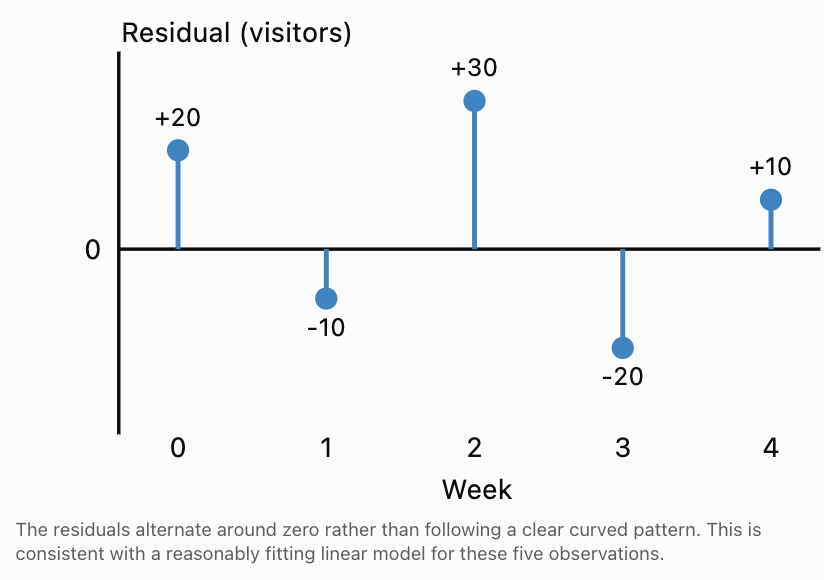
Interpreting Residual Patterns
A useful model should generally produce residuals that are small relative to the scale of the data.
We also examine whether residuals follow a pattern.
-
Residuals scattered around zero suggest the model captures the main trend.
-
A curved residual pattern suggests the chosen function may be missing curvature.
-
Residuals that increase in magnitude suggest changing prediction accuracy.
-
A single unusually large residual may indicate an outlier or measurement problem.
Residuals alone cannot prove that a model is correct, but they are valuable for identifying weaknesses.
Measuring Model Accuracy
Several numerical measures can be used to compare models.
Mean Absolute Error (MAE)
The mean absolute error measures the average size of the prediction errors.
where n is the number of observations.
For the visitor data:
Absolute residuals:
20, 10, 30, 20, 10
MAE = (20 + 10 + 30 + 20 + 10)/5
MAE = 90/5
MAE = 18 visitors.
This means the model's predictions differ from the observations by an average of 18 visitors.
Mean Squared Error (MSE)
Mean squared error gives more weight to large errors.
For the same data:
MSE = (400 + 100 + 900 + 400 + 100)/5
MSE = 1900/5
MSE = 380 visitors².
Root Mean Squared Error (RMSE)
RMSE is the square root of MSE:
RMSE = √380
RMSE ≈ 19.49 visitors.
RMSE has the same units as the original output variable, making it easier to interpret than MSE.
Coefficient of Determination (R²)
R² measures how much of the variation in the observed outputs is accounted for by a model relative to predicting their mean.
For a model evaluated on a dataset:
where ȳ is the mean observed output.
Values close to 1 often indicate a strong fit on the evaluated dataset.
However, R² does not establish that a model is scientifically correct, nor does it guarantee accurate future predictions. R² can also be negative when predictions are worse than using the observed mean.
Worked Example 7: Comparing Two Models
Suppose the following data describe a company's revenue over five years.
|
Year t |
Revenue ($ thousands) |
|---|---|
|
0 |
10 |
|
1 |
15 |
|
2 |
22 |
|
3 |
31 |
|
4 |
42 |
We consider two models.
Model A: Linear
L(t) = 8t + 8
Model B: Quadratic
Q(t) = t² + 4t + 10
Calculate predictions.
|
t |
Observed |
Linear prediction |
Quadratic prediction |
|---|---|---|---|
|
0 |
10 |
8 |
10 |
|
1 |
15 |
16 |
15 |
|
2 |
22 |
24 |
22 |
|
3 |
31 |
32 |
31 |
|
4 |
42 |
40 |
42 |
Evaluate Model A.
Residuals:
2, −1, −2, −1, 2
MAE:
(2 + 1 + 2 + 1 + 2)/5 = 1.6
Evaluate Model B.
All residuals are zero.
MAE = 0
Therefore, Model B fits the observed data exactly.
Does this guarantee Model B is the better long-term model?
No.
The quadratic model perfectly fits these five observations, but future revenue may be affected by competition, economic conditions, market saturation, or other factors.
An exact fit to past data does not guarantee accurate extrapolation.
When evaluating models, consider mathematical accuracy, simplicity, assumptions, and whether the relationship makes sense in context.
Interpolation and Extrapolation
Mathematical models are often used to estimate values that were not directly measured.
There are two important types of prediction.
Interpolation means predicting within the range of observed input values.
Extrapolation means predicting outside the observed range.
Suppose measurements were collected for x-values between 0 and 10.
Predicting at x = 6.5 is interpolation.
Predicting at x = 25 is extrapolation.
Extrapolation is generally more uncertain because the relationship may change beyond the observed range.
For example, a quadratic model of company revenue might fit five years of data but predict unrealistic revenue after 50 years.
A good modelling report should clearly distinguish between predictions supported by observed data and predictions that extend beyond it.
Solving Real-World Problems Using Models
After creating and evaluating a model, we can use it to answer practical questions.
These often involve solving equations, identifying maximum or minimum values, or comparing different functions.
Worked Example 8: Break-Even Analysis
A company sells each product for $40.
Its total cost is:
C(x) = 500 + 15x
Revenue is:
R(x) = 40x
Profit is revenue minus cost:
P(x) = R(x) − C(x)
P(x) = 40x − (500 + 15x)
P(x) = 25x − 500
Find the break-even quantity.
At break-even:
P(x) = 0
25x − 500 = 0
25x = 500
x = 20
The company breaks even when it sells 20 items.
Find the profit from 80 items.
P(80) = 25(80) − 500
= 2000 − 500
= $1,500
Interpretation: Selling more than 20 items produces a positive profit under this model.
Worked Example 9: Solving a Rational Cost Model
A manufacturer's average cost per item is:
A(x) = 900/x + 18
The company wants average cost to be no more than $30.
Solve:
900/x + 18 ≤ 30
For the practical domain x > 0:
900/x ≤ 12
Multiply both sides by positive x:
900 ≤ 12x
x ≥ 75
Therefore, the company must produce at least 75 items to achieve an average cost of $30 or less.
The positivity of x matters when multiplying an inequality by x.
Worked Example 10: Optimizing a Polynomial Model
A farmer has 80 metres of fencing to create a rectangular enclosure along a straight wall. The wall forms one side, so fencing is required for only three sides.
Let x be the width perpendicular to the wall.
The two widths use 2x metres of fencing.
The remaining fenced length is:
80 − 2x
Area:
A(x) = x(80 − 2x)
Expand:
A(x) = −2x² + 80x
This is a downward-opening quadratic.
Find the maximum area.
Vertex x-coordinate:
x = −80/[2(−2)]
x = 20
Length:
80 − 2(20) = 40
Maximum area:
A(20) = 20 × 40
= 800 m²
Conclusion: The farmer should construct an enclosure 20 metres wide and 40 metres long to maximize area.
The practical domain is 0 < x < 40.
Evaluating the Limitations of Models
Every mathematical model relies on assumptions.
For example:
A projectile model may ignore air resistance.
A production-cost model may assume fixed costs and constant material prices.
A population model may assume stable environmental conditions.
A travel-time model may assume constant speed.
These assumptions simplify calculations, but they may reduce accuracy.
Questions to Ask When Evaluating a Model
-
Does the model match the observed data reasonably well?
-
Are its parameters meaningful?
-
Does it predict realistic values?
-
Are the domain and range appropriate for the situation?
-
Are there outliers or systematic residual patterns?
-
Is the model unnecessarily complicated?
-
Are predictions being made outside the observed data?
-
Could important external factors change the relationship?
A useful model is not necessarily the most complicated model. Often, a simpler model is preferable when it explains the data adequately and is easier to interpret.
Common Mistakes
Mistake 1: Choosing a Model Based Only on Its Graph
A graph may resemble a quadratic curve, but this does not prove the relationship is quadratic.
Examine the variables, data patterns, and underlying mathematical relationship.
Mistake 2: Assuming All Curved Relationships Are Quadratic
A curved relationship could be cubic, rational, exponential, logarithmic, or another function type.
For example, travel time for a fixed distance follows t = d/v, not a quadratic model.
Mistake 3: Ignoring Units
A parameter has meaning only when interpreted with appropriate units.
In C(x) = 5x + 100, the coefficient 5 might represent dollars per item, while 100 represents dollars.
Mistake 4: Using an Incorrect Domain
A production quantity cannot be negative.
A time after launch cannot be negative.
A physical length must be positive.
The mathematical domain and practical domain may be different.
Mistake 5: Confusing a Perfect Fit with a Reliable Model
A polynomial can fit a small number of data points exactly while giving unrealistic predictions outside the observed range.
Mistake 6: Confusing Residual Signs
Residual = Observed − Predicted.
A positive residual means the model underestimated the observed value.
A negative residual means the model overestimated it.
Mistake 7: Ignoring Asymptotes in Rational Models
An asymptote may represent an important limiting value.
For A(x) = 500/x + 12, the horizontal asymptote y = 12 represents the variable cost per item.
Mistake 8: Treating Predictions as Certainties
Models are simplified representations of reality. Their predictions depend on assumptions, data quality, and the stability of the relationship.
Mistake 9: Forgetting to Interpret the Answer
Solving x = 75 is not enough.
A complete conclusion should explain that 75 items must be produced to meet the target average cost.
Key Terms
-
Mathematical Model: A mathematical representation of a real-world situation.
-
Polynomial Model: A model using a polynomial function.
-
Rational Model: A model using a quotient of polynomial functions.
-
Independent Variable: The input quantity.
-
Dependent Variable: The output quantity.
-
Parameter: A constant in a model that controls its behaviour.
-
Linear Model: A model with a constant rate of change.
-
Quadratic Model: A second-degree polynomial model.
-
Cubic Model: A third-degree polynomial model.
-
Inverse Variation: A relationship where one quantity is proportional to the reciprocal of another.
-
Regression: A method of estimating a model's parameters from data.
-
Residual: The difference between an observed value and a predicted value.
-
Mean Absolute Error (MAE): The average absolute prediction error.
-
Mean Squared Error (MSE): The average squared prediction error.
-
Root Mean Squared Error (RMSE): The square root of MSE.
-
Coefficient of Determination (R²): A measure comparing prediction error with variation around the observed mean.
-
Interpolation: Estimating a value within the observed input range.
-
Extrapolation: Estimating a value outside the observed input range.
-
Asymptote: A line approached by a graph in a limiting situation.
-
Practical Domain: The input values that make sense in the real-world context.
-
Break-Even Point: The quantity at which revenue equals cost.
-
Optimization: Finding the greatest or least possible value under given conditions.
-
Assumption: A simplifying condition accepted when constructing a model.
-
Model Validation: Evaluating how well a model performs against relevant observations, preferably including data not used to fit it.
Key Takeaways
-
Mathematical modelling connects real-world situations with mathematical functions.
-
Polynomial models are useful for relationships involving constant rates, area, volume, motion, and curved trends.
-
Rational models are useful for ratios, rates, average costs, and inverse relationships.
-
Data tables and graphs help identify possible models.
-
Constant first differences suggest a linear relationship for equally spaced inputs.
-
Constant second differences suggest a quadratic relationship under suitable conditions.
-
Model parameters should be interpreted using real-world units.
-
Residuals measure differences between observed and predicted values.
-
MAE, MSE, RMSE, and R² can help evaluate model accuracy.
-
A model that fits past data perfectly may still make poor future predictions.
-
Interpolation is generally more reliable than extrapolation.
-
Practical domains may be more restricted than mathematical domains.
-
Models can be used to find break-even points, optimize quantities, and make predictions.
-
Good mathematical modelling requires interpretation, evaluation, and awareness of limitations.
Check Your Understanding
Question 1: Choosing a Model
Choose a suitable polynomial or rational model for each situation and explain why.
a) The height of a ball thrown vertically upward.
b) The time needed to travel 300 km at different constant speeds.
c) The area of a square as its side length changes.
d) The average cost per item when there is a fixed production cost.
Question 2: Identifying a Linear Model
The following data show the cost of a service.
|
Hours |
Cost ($) |
|---|---|
|
1 |
45 |
|
2 |
70 |
|
3 |
95 |
|
4 |
120 |
Find a linear model and interpret its parameters.
Question 3: Creating a Quadratic Model
A quadratic function passes through:
(0, 3), (1, 8), and (2, 11).
Find an equation of the form:
f(x) = ax² + bx + c
Question 4: Creating a Rational Model
The average cost of producing x items follows:
A(x) = a/x + b
Given:
A(20) = 40
A(40) = 30
Find a and b, then calculate A(100).
Question 5: Evaluating Residuals
A model predicts the following values:
|
Observed |
Predicted |
|---|---|
|
12 |
10 |
|
18 |
20 |
|
25 |
24 |
|
31 |
34 |
a) Calculate the residuals.
b) Calculate the MAE.
c) Explain what the MAE means.
Question 6: Interpolation and Extrapolation
A scientist collects data for temperatures between 10°C and 40°C.
Classify the following predictions as interpolation or extrapolation.
a) Predicting at 25°C.
b) Predicting at 60°C.
c) Predicting at 5°C.
Which predictions require greater caution?
Question 7: Interpreting Parameters
A company uses:
C(x) = 750 + 18x
where x is the number of items produced.
a) What does 750 represent?
b) What does 18 represent?
c) Calculate the cost of producing 150 items.
d) Write an average-cost function.
Question 8: Solving a Rational Model
A factory's average cost is:
A(x) = 1200/x + 25
How many items must be produced for average cost to be no more than $40?
Question 9: Optimization
A rectangular garden has a perimeter of 60 m.
a) Write an area function in terms of one side length x.
b) Find the maximum area.
c) Determine the garden dimensions that produce this area.
Question 10: Challenge — Comparing Two Models
Two companies have average-cost functions:
A(x) = 300/x + 18
B(x) = 600/x + 15
a) Find the production quantity where average costs are equal.
b) Calculate the average cost at that quantity.
c) Determine which company is cheaper for 50 items.
d) Determine which company is cheaper for 200 items.
e) Explain why the preferred company changes as production increases.
Fully Worked Answers
Answer 1: Choosing Models
a) Quadratic polynomial.
Under constant gravitational acceleration, height changes quadratically with time.
b) Rational.
Time = Distance / Speed, so t(v) = 300/v.
c) Quadratic polynomial.
A(s) = s².
d) Rational.
Average cost is total cost divided by production quantity.
Answer 2: Linear Model
The cost increases by $25 for each additional hour.
Therefore:
m = 25
Use:
C = 25h + b
Substitute (1, 45):
45 = 25 + b
b = 20
Final model:
C = 25h + 20
The hourly charge is $25.
The fixed fee is $20.
Answer 3: Quadratic Model
Use:
f(x) = ax² + bx + c
At (0, 3):
c = 3
At (1, 8):
a + b + 3 = 8
a + b = 5
At (2, 11):
4a + 2b + 3 = 11
4a + 2b = 8
2a + b = 4
Subtract:
(2a + b) − (a + b) = 4 − 5
a = −1
Then:
−1 + b = 5
b = 6
Final model:
f(x) = −x² + 6x + 3
Answer 4: Rational Model
Given:
A(x) = a/x + b
Using A(20) = 40:
40 = a/20 + b
Using A(40) = 30:
30 = a/40 + b
Subtract:
10 = a/40
a = 400
Substitute:
40 = 400/20 + b
40 = 20 + b
b = 20
Final model:
A(x) = 400/x + 20
At x = 100:
A(100) = 400/100 + 20
= 4 + 20
= $24 per item.
Answer 5: Residuals
Residual = Observed − Predicted.
Residuals:
12 − 10 = +2
18 − 20 = −2
25 − 24 = +1
31 − 34 = −3
Absolute residuals:
2, 2, 1, 3
MAE = (2 + 2 + 1 + 3)/4
MAE = 8/4
MAE = 2.
The model's predictions differ from the observations by an average of 2 units.
Answer 6: Interpolation and Extrapolation
Observed range: 10°C to 40°C.
a) 25°C is interpolation.
b) 60°C is extrapolation.
c) 5°C is extrapolation.
Predictions at 60°C and 5°C require greater caution because they are outside the observed range.
Answer 7: Interpreting Parameters
Given:
C(x) = 750 + 18x
a) 750 represents the fixed cost of $750.
b) 18 represents the variable cost of $18 per item.
c) At 150 items:
C(150) = 750 + 18(150)
= 750 + 2700
= $3,450
d) Average cost:
A(x) = C(x)/x
A(x) = (750 + 18x)/x
Final model:
A(x) = 750/x + 18
for x > 0.
Answer 8: Rational Model
Given:
A(x) = 1200/x + 25
We require:
1200/x + 25 ≤ 40
Subtract 25:
1200/x ≤ 15
Since x > 0:
1200 ≤ 15x
x ≥ 80
Answer: At least 80 items must be produced.
Answer 9: Optimization
Perimeter:
2L + 2W = 60
Divide by 2:
L + W = 30
Let W = x.
Then:
L = 30 − x
Area:
A(x) = x(30 − x)
Expand:
A(x) = −x² + 30x
The parabola opens downward.
Vertex:
x = −30/[2(−1)]
x = 15
Length:
30 − 15 = 15
Maximum area:
15 × 15 = 225 m²
Answer: A 15 m by 15 m square gives the maximum area of 225 m².
Answer 10: Comparing Companies
Given:
A(x) = 300/x + 18
B(x) = 600/x + 15
a) Equal average costs
300/x + 18 = 600/x + 15
18 − 15 = 600/x − 300/x
3 = 300/x
3x = 300
x = 100
b) Average cost at 100 items
A(100) = 300/100 + 18
= $21
B(100) = 600/100 + 15
= $21
c) At 50 items
A(50) = 300/50 + 18 = $24
B(50) = 600/50 + 15 = $27
Company A is cheaper.
d) At 200 items
A(200) = 300/200 + 18 = $19.50
B(200) = 600/200 + 15 = $18
Company B is cheaper.
e) Interpretation
Company A has lower fixed costs but higher variable costs.
Company B has higher fixed costs but lower variable costs.
At low production quantities, Company A's lower fixed costs make it cheaper.
At high production quantities, Company B's lower variable cost becomes more important.
The crossover occurs at 100 items.
This completes Real-World Modelling, covering all five learning targets: selecting polynomial and rational models, constructing models from data, evaluating accuracy, interpreting parameters, and solving practical problems using mathematical functions.