Applications and Function Analysis
| Hệ thống: | Young Education |
| Khoá học: | Polynomial and Rational Functions |
| Book: | Applications and Function Analysis |
| Được in bởi: | Guest user |
| Ngày: | Thứ Hai, 9 tháng 11 2026, 4:40 PM |
1. Comparing Polynomial and Rational Functions
Learning outcomes
- I can compare the characteristics of polynomial and rational functions.
- I can distinguish between their graphs.
- I can compare domains and ranges.
- I can identify similarities and differences.
- I can choose appropriate models for different situations.
Introduction
Mathematical functions help us describe relationships between quantities, recognize patterns, predict outcomes, and model real-world situations.
Two important families of functions are polynomial functions and rational functions.
Polynomial functions are used to model relationships such as the height of a projectile, the area of a shape, and changes in revenue or profit. Their graphs are continuous, smooth curves without breaks or vertical asymptotes.
Rational functions are especially useful when one quantity depends on another through division. They can model average costs, travel time, concentration, work rates, and inverse relationships. Their graphs may contain holes, vertical asymptotes, horizontal asymptotes, and separate branches.
Although these two families of functions share many algebraic properties, they also behave differently in important ways.
Understanding these similarities and differences helps us select suitable mathematical models, interpret graphs correctly, and recognize the limitations of mathematical predictions.
In this lesson, we will compare the algebraic forms, graphs, domains, ranges, intercepts, asymptotes, and real-world applications of polynomial and rational functions.
What Is a Polynomial Function?
A polynomial function is a function that can be written as:
f(x) = aₙxⁿ + aₙ₋₁xⁿ⁻¹ + ... + a₂x² + a₁x + a₀
where:
-
The coefficients are real numbers.
-
The exponents are nonnegative integers.
-
The leading coefficient aₙ is nonzero for a polynomial of degree n.
Examples include:
-
f(x) = 3x + 2
-
f(x) = x² − 4x + 3
-
f(x) = −2x³ + 5x
-
f(x) = x⁴ − 3x² + 1
Polynomial functions can be classified by their degree.
|
Degree |
Type |
Example |
|---|---|---|
|
0 |
Constant |
f(x) = 5 |
|
1 |
Linear |
f(x) = 2x + 1 |
|
2 |
Quadratic |
f(x) = x² − 4 |
|
3 |
Cubic |
f(x) = x³ − 2x |
|
4 |
Quartic |
f(x) = x⁴ − 5x² |
Important Characteristics of Polynomial Functions
-
Their natural domain is all real numbers.
-
Their graphs are continuous and smooth.
-
They do not have holes or vertical asymptotes.
-
They may have turning points.
-
Their end behaviour depends on the degree and leading coefficient.
-
They can have multiple real x-intercepts.
A polynomial graph can change direction, cross the x-axis, or touch the x-axis without crossing it.
What Is a Rational Function?
A rational function is a function that can be written as:
where P(x) and Q(x) are polynomials and Q(x) is not the zero polynomial.
Examples include:
-
f(x) = 1/x
-
f(x) = (x + 2)/(x − 3)
-
f(x) = (x² − 4)/(x + 1)
-
f(x) = (2x² + 1)/(x² − 9)
Important Characteristics of Rational Functions
-
Their domain excludes values that make the denominator zero.
-
Their graphs may have vertical asymptotes.
-
They may have horizontal, oblique, or higher-degree polynomial asymptotes.
-
They may contain holes.
-
Their graphs can consist of separate branches.
-
Their end behaviour depends on the relative degrees of the numerator and denominator.
An Important Mathematical Connection
Every polynomial function is also a rational function because it can be written with denominator 1.
For example:
f(x) = x² + 3x + 2
can be written as:
Therefore, polynomial functions form a subset of rational functions.
However, rational functions such as 1/x are not polynomial functions.
Comparing the Two Function Families
|
Characteristic |
Polynomial functions |
|
|---|---|---|
|
General form |
Sum of nonnegative integer powers of x |
Ratio of two polynomials |
|
Natural domain |
All real numbers |
All real numbers except denominator zeros |
|
Continuity |
Continuous everywhere |
Continuous wherever defined |
|
Graph shape |
Smooth, unbroken |
May have branches or holes |
|
Vertical asymptotes |
None |
Possible |
|
Horizontal asymptotes |
Only constant polynomials |
Common, but not guaranteed |
|
Oblique asymptotes |
A nonconstant polynomial is its own line only when linear |
Possible |
|
x-intercepts |
Zeros of the polynomial |
Valid zeros of the numerator |
|
y-intercept |
Always exists |
Exists if x = 0 is in the domain |
|
Turning points |
Possible |
Possible |
|
Typical applications |
Area, trajectories, profit, growth |
Rates, ratios, average cost, inverse relationships |
Important: The two families overlap. Some rational functions simplify to polynomials with holes, and some rational functions are exactly polynomial functions.
Comparing Their Graphs
Graph shape is often the easiest way to distinguish polynomial functions from rational functions.
Polynomial Graphs
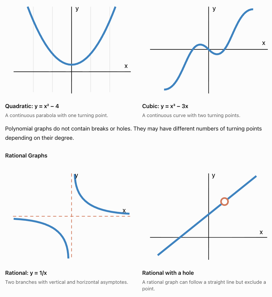
A graph with a vertical asymptote or a hole cannot be the graph of a polynomial function defined on all real numbers.
However, a smooth-looking graph alone does not prove that a function is polynomial. Some rational functions have no real denominator zeros and are continuous everywhere.
Comparing Domains
The domain of a function is the set of all input values for which the function is defined.
Domain of Polynomial Functions
Every polynomial function has the natural domain:
All real numbers.
In interval notation:
For example:
f(x) = x² − 5x + 6
We can substitute any real number for x without creating an undefined operation.
Therefore, the domain is all real numbers.
Domain of Rational Functions
For rational functions, we must exclude values that make the denominator zero.
Worked Example 1: Comparing Domains
Compare:
f(x) = x² − 9
g(x) = (x² − 9)/(x − 3)
Step 1: Find the polynomial domain.
f(x) is a polynomial.
Domain: all real numbers.
Step 2: Find the rational domain.
For g(x):
x − 3 = 0
x = 3
Therefore:
Domain: x ≠ 3.
Step 3: Simplify the rational function.
g(x) = (x − 3)(x + 3)/(x − 3)
g(x) = x + 3, where x ≠ 3.
Conclusion: Both functions have polynomial expressions associated with them, but the rational function has a missing point at (3, 6). The original polynomial f(x) = x² − 9 is defined at x = 3.
This example demonstrates that simplification does not eliminate original domain restrictions.
Comparing Ranges
The range of a function is the set of all possible output values.
Unlike the domain, the range often requires analyzing the graph, finding extrema, or solving an equation for x.
Range of Polynomial Functions
Different polynomial functions have different ranges.
|
Polynomial |
Range |
|---|---|
|
f(x) = 2x + 1 |
All real numbers |
|
f(x) = x² |
y ≥ 0 |
|
f(x) = −x² + 4 |
y ≤ 4 |
|
f(x) = x³ |
All real numbers |
|
f(x) = x⁴ + 2 |
y ≥ 2 |
For example:
f(x) = x² + 3
Since x² ≥ 0:
x² + 3 ≥ 3
Therefore:
Range: [3, ∞)
Range of Rational Functions
Rational functions may exclude certain output values because of asymptotes, holes, or other restrictions.
Consider:
g(x) = 1/x
The function can never equal zero because its numerator is 1.
Therefore:
Range: all real numbers except 0.
In interval notation:
Worked Example 2: Comparing Ranges
Compare:
f(x) = x²
g(x) = 1/(x² + 1)
Polynomial:
f(x) = x²
The minimum value occurs at x = 0.
f(0) = 0
As |x| increases, f(x) increases without bound.
Range:
[0, ∞)
Rational function:
g(x) = 1/(x² + 1)
Since x² ≥ 0:
x² + 1 ≥ 1
Therefore:
0 < 1/(x² + 1) ≤ 1
The maximum occurs at x = 0:
g(0) = 1
As |x| becomes very large, g(x) approaches zero but never reaches it.
Range:
(0, 1]
Conclusion: The polynomial has a minimum and no maximum, while the rational function has a maximum and approaches a lower bound it never reaches.
A Useful Warning About Horizontal Asymptotes
A horizontal asymptote is not automatically an excluded range value.
For example:
h(x) = (x² − 1)/(x² + 1)
has horizontal asymptote y = 1, and the graph never reaches 1.
But:
k(x) = (x² − 1)/(x² + 2)
also has horizontal asymptote y = 1 and never reaches it.
Other rational functions can cross their horizontal asymptotes. To determine the range, we must analyze the actual outputs rather than assuming the asymptote is excluded.
Comparing Intercepts
Both polynomial and rational functions can have x- and y-intercepts.
Polynomial Intercepts
For a polynomial function:
f(x) = P(x)
x-intercepts are found by solving:
P(x) = 0
The y-intercept is found by calculating:
f(0)
Every polynomial function has a y-intercept because its domain includes x = 0.
Rational Intercepts
For:
g(x) = P(x)/Q(x)
x-intercepts occur where:
P(x) = 0
provided Q(x) ≠ 0.
The y-intercept is g(0), provided Q(0) ≠ 0.
Worked Example 3: Comparing Intercepts
Compare:
f(x) = x² − 4
g(x) = (x² − 4)/(x + 2)
Polynomial:
Factor:
f(x) = (x − 2)(x + 2)
x-intercepts:
(−2, 0) and (2, 0)
y-intercept:
f(0) = −4
Therefore, (0, −4).
Rational function:
Factor:
g(x) = (x − 2)(x + 2)/(x + 2)
Simplify:
g(x) = x − 2, where x ≠ −2.
x-intercept:
(2, 0)
y-intercept:
g(0) = −2
Therefore, (0, −2).
Hole:
At x = −2, the simplified expression gives:
y = −2 − 2 = −4
Hole at (−2, −4).
Conclusion: The polynomial has two x-intercepts, while the rational function has one x-intercept and a hole.
Comparing End Behaviour
End behaviour describes what happens to a function as x approaches positive or negative infinity.
Polynomial End Behaviour
The degree and leading coefficient determine polynomial end behaviour.
|
Degree and leading coefficient |
Left end |
Right end |
|---|---|---|
|
Even degree, positive |
Up |
Up |
|
Even degree, negative |
Down |
Down |
|
Odd degree, positive |
Down |
Up |
|
Odd degree, negative |
Up |
Down |
For example:
f(x) = 2x⁴ − 3x² + 1
The leading term is 2x⁴.
Because the degree is even and the leading coefficient is positive, both ends of the graph rise.
Rational End Behaviour
Rational functions depend on the relative degrees of numerator and denominator.
For:
g(x) = P(x)/Q(x)
-
If the numerator degree is smaller, the horizontal asymptote is y = 0.
-
If the degrees are equal, the horizontal asymptote is the ratio of leading coefficients.
-
If the numerator degree is exactly one greater, there is an oblique asymptote.
-
If the numerator degree exceeds the denominator degree by two or more, there may be a higher-degree polynomial asymptote.
Worked Example 4: Comparing End Behaviour
Compare:
f(x) = x² + 2
g(x) = (x² + 2)/(x² + 1)
Polynomial:
As x approaches positive or negative infinity:
f(x) approaches positive infinity.
Rational function:
Both numerator and denominator have degree 2.
The ratio of leading coefficients is:
1/1 = 1
Therefore, the horizontal asymptote is y = 1.
We can rewrite:
g(x) = 1 + 1/(x² + 1)
As |x| increases, the second term approaches zero.
Therefore, g(x) approaches 1 from above.
Conclusion: The polynomial grows without bound, while the rational function approaches a finite value.
Comparing Continuity and Asymptotes
A polynomial function is continuous everywhere on the real number line.
This means that its graph can be drawn without lifting the pencil, and there are no holes, jumps, or vertical asymptotes.
Rational functions are continuous wherever their denominators are nonzero, but may be undefined at certain values.
Worked Example 5: A Rational Function with No Real Discontinuities
Consider:
g(x) = 1/(x² + 4)
The denominator is always positive because:
x² ≥ 0
Therefore:
x² + 4 ≥ 4
The denominator never equals zero.
So:
-
Domain: all real numbers.
-
No vertical asymptotes.
-
No holes.
-
Continuous everywhere.
-
Horizontal asymptote: y = 0.
-
Range: (0, 1/4].
This shows that not all rational functions have breaks in their graphs.
Similarities and Differences
Polynomial and rational functions have several important similarities.
Both can be evaluated by substitution, represented using tables and graphs, and analyzed using algebraic techniques. Both can have intercepts, turning points, increasing and decreasing intervals, and symmetry. Both can model real-world relationships.
Their most important differences concern domain restrictions, continuity, asymptotes, and end behaviour.
A polynomial's natural domain is always all real numbers, while a rational function may have excluded inputs. A polynomial is continuous everywhere, while a rational function may contain holes or vertical asymptotes.
Nevertheless, because every polynomial is also rational, these differences describe typical non-polynomial rational functions rather than an absolute separation between the two families.
Choosing Appropriate Mathematical Models
The choice between a polynomial and rational model depends on the relationship between the quantities.
A good mathematical model should:
-
Represent the main pattern in the situation.
-
Have a domain that makes sense in context.
-
Produce reasonable predictions.
-
Reflect important physical or mathematical restrictions.
-
Be simple enough to interpret and use.
When to Use Polynomial Models
Polynomial models are often appropriate when a quantity changes according to sums of powers of another quantity.
Examples include:
-
Projectile motion with constant gravitational acceleration.
-
Area and volume calculations.
-
Revenue and profit relationships.
-
Curved trends that can be approximated using polynomial regression.
When to Use Rational Models
Rational models are often appropriate when a quantity involves division by a changing variable.
Examples include:
-
Time required to travel a fixed distance.
-
Average production cost.
-
Concentration and dilution.
-
Work rates.
-
Inverse variation.
-
Electrical relationships.
Real-World Application 1: Projectile Motion
Suppose a ball is thrown upward from a platform.
Its height in metres after t seconds is modelled by:
h(t) = −5t² + 20t + 2
This is a quadratic polynomial function.
Why is a polynomial model appropriate?
The equation describes vertical motion under constant gravitational acceleration, ignoring air resistance.
Find the maximum height.
The vertex occurs at:
t = −b/(2a)
Here:
a = −5, b = 20
Therefore:
t = −20/[2(−5)] = 2 seconds
Substitute:
h(2) = −5(2²) + 20(2) + 2
= −20 + 40 + 2
= 22
Maximum height: 22 m.
The mathematical polynomial is defined for all real t, but the physical model is meaningful only during the flight, from t = 0 until the ball reaches the ground.
Real-World Application 2: Average Production Cost
A company has a fixed cost of $800 and a variable cost of $12 per item.
The total cost is:
C(x) = 800 + 12x
This is a linear polynomial function.
However, the average cost per item is:
Simplify:
A(x) = 800/x + 12
This is a non-polynomial rational function.
|
Items produced |
Total cost |
Average cost |
|---|---|---|
|
20 |
$1,040 |
$52 |
|
50 |
$1,400 |
$28 |
|
100 |
$2,000 |
$20 |
|
200 |
$3,200 |
$16 |
|
400 |
$5,600 |
$14 |
As production increases, total cost increases linearly, but average cost decreases toward $12.
Why is a rational model appropriate for average cost?
Because average cost is calculated by dividing total cost by the number of items.
The rational function has a horizontal asymptote at y = 12, representing the variable cost per item.
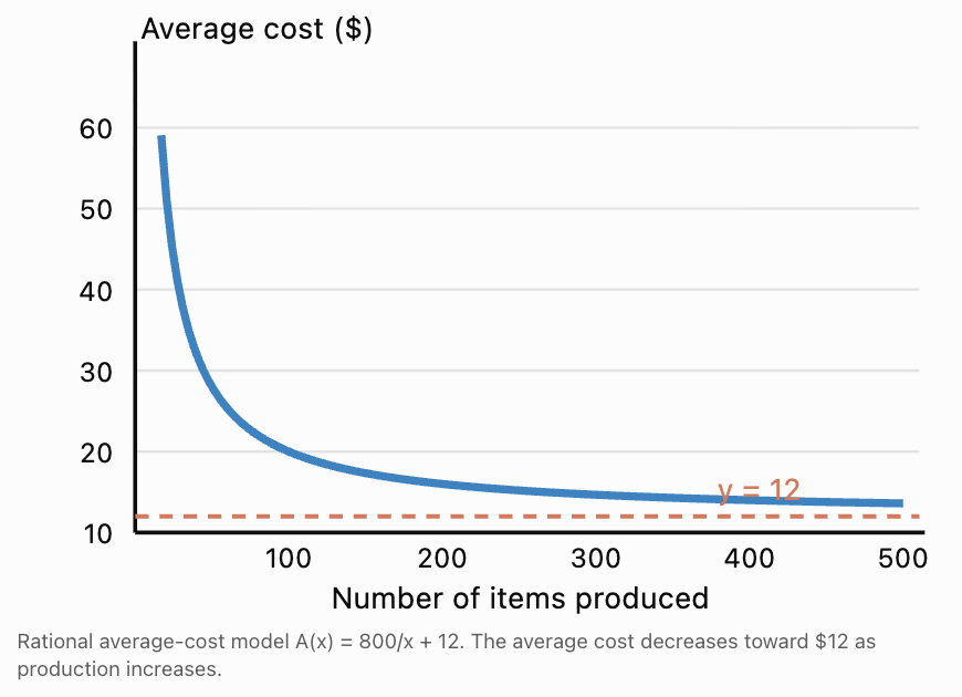
Real-World Application 3: Travel Time
Suppose a car travels a fixed distance of 240 km.
The journey time is:
t(v) = 240/v
where v is speed in km/h.
This is a rational function.
|
Speed (km/h) |
Time (hours) |
|---|---|
|
40 |
6 |
|
60 |
4 |
|
80 |
3 |
|
100 |
2.4 |
|
120 |
2 |
Why not use a linear polynomial model?
Because doubling the speed halves the time, rather than reducing it by a constant amount.
The relationship is inverse variation, which is naturally represented by a rational function.
The physical domain is v greater than zero, with additional practical limits such as road speed restrictions.
Real-World Application 4: Comparing Two Models for the Same Situation
Suppose a business sells x items at $25 each and incurs a fixed cost of $500 plus $10 per item.
Revenue:
R(x) = 25x
Cost:
C(x) = 500 + 10x
Profit:
P(x) = R(x) − C(x)
P(x) = 15x − 500
This is a polynomial function.
However, profit per item is:
Simplify:
p(x) = 15 − 500/x
This is a rational function for x greater than zero.
The polynomial model describes total profit, while the rational model describes profit per item.
The same business situation may require different function families depending on the question being asked.
Evaluating the Reasonableness of a Model
A mathematical model may describe a pattern accurately over one interval but become unrealistic outside that interval.
For example, a polynomial model of population growth might eventually predict negative population values or implausibly rapid growth.
A rational model of average cost might approach a horizontal asymptote, but real production costs may change because of material shortages, capacity limits, or inflation.
Before using a model to make predictions, consider whether its assumptions remain reasonable over the intended domain.
Common Mistakes
Mistake 1: Assuming Polynomial and Rational Functions Are Completely Separate Categories
Every polynomial can be written as a rational function with denominator 1.
Therefore, all polynomial functions are rational functions, but not all rational functions are polynomial functions.
Mistake 2: Assuming Every Rational Function Has a Vertical Asymptote
The function f(x) = 1/(x² + 1) has no vertical asymptotes because its denominator never equals zero for real x.
Mistake 3: Forgetting Domain Restrictions After Simplifying
(x² − 4)/(x − 2) simplifies to x + 2, but x = 2 remains excluded.
The graph has a hole, unlike the complete polynomial line y = x + 2.
Mistake 4: Assuming Every Rational Function Has a Restricted Domain
Some rational functions, such as 1/(x² + 1), are defined for all real x.
Mistake 5: Assuming Horizontal Asymptotes Cannot Be Crossed
Horizontal asymptotes describe end behaviour. A rational graph may cross a horizontal asymptote at a finite input value.
Mistake 6: Confusing Domain and Range
Domain refers to permitted x-values.
Range refers to possible y-values.
For f(x) = 1/x, both exclude zero, but this is not true for every rational function.
Mistake 7: Choosing a Model Only Because Its Graph Looks Similar
A curve may resemble a polynomial or rational graph over a short interval.
The underlying relationship, domain, asymptotic behaviour, and physical meaning should also guide the model choice.
Key Terms
-
Polynomial Function: A function expressed as a sum of terms containing nonnegative integer powers of a variable.
-
Rational Function: A function expressed as the quotient of two polynomials, with a denominator that is not the zero polynomial.
-
Degree: The highest exponent of a variable in a polynomial.
-
Leading Coefficient: The coefficient of the highest-degree term.
-
Domain: The set of all permitted input values.
-
Range: The set of all possible output values.
-
Continuous Function: A function whose graph has no breaks at points within its domain.
-
Discontinuity: A point where a function is not continuous.
-
Hole: A missing point caused by a removable discontinuity.
-
Vertical Asymptote: A vertical line approached by a graph as function values increase or decrease without bound.
-
Horizontal Asymptote: A horizontal line approached by a graph as x tends toward positive or negative infinity.
-
Oblique Asymptote: A nonhorizontal straight line approached by a graph at infinity.
-
x-Intercept: A point where a graph crosses or touches the x-axis.
-
y-Intercept: A point where a graph intersects the y-axis.
-
Turning Point: A point where a function changes from increasing to decreasing or vice versa.
-
End Behaviour: The behaviour of a function as x approaches positive or negative infinity.
-
Mathematical Model: A mathematical representation of a real-world relationship.
-
Inverse Variation: A relationship in which one quantity is proportional to the reciprocal of another.
Key Takeaways
-
Polynomial functions contain sums of nonnegative integer powers of variables.
-
Rational functions are ratios of polynomials.
-
Every polynomial function is also a rational function, but not every rational function is a polynomial.
-
Polynomial functions have all real numbers as their natural domain.
-
Rational functions may have excluded values, holes, or vertical asymptotes.
-
Polynomial graphs are continuous and smooth everywhere.
-
Rational functions are continuous wherever their denominators are nonzero.
-
Both families can have intercepts, turning points, and useful real-world applications.
-
Polynomial end behaviour depends on degree and leading coefficient.
-
Rational end behaviour depends on the relative degrees of numerator and denominator.
-
Ranges must be determined from the actual outputs of the function.
-
Polynomial models are often suitable for trajectories, area, revenue, and profit.
-
Rational models are often suitable for rates, ratios, inverse variation, and average costs.
-
The most appropriate model depends on the mathematical relationship and the real-world context.
Check Your Understanding
Question 1: Classifying Functions
Classify each function as polynomial, rational but not polynomial, or neither.
a) f(x) = 3x² − 5x + 2
b) g(x) = 4/(x − 1)
c) h(x) = (x² + 1)/(x² + 4)
d) p(x) = √x + 3
Question 2: Comparing Domains
Find the natural domain of each function.
a) f(x) = x² − 16
b) g(x) = (x² − 16)/(x − 4)
Explain the difference.
Question 3: Comparing Ranges
Find the range of each function.
a) f(x) = x² + 2
b) g(x) = 1/(x² + 2)
Question 4: Comparing Intercepts
Find the x- and y-intercepts of:
a) f(x) = x² − 9
b) g(x) = (x² − 9)/(x + 3)
Question 5: Comparing Graph Features
Consider:
f(x) = x² + 1
g(x) = 1/(x² + 1)
For each function, identify:
a) Domain.
b) Range.
c) Any vertical asymptotes.
d) Horizontal asymptotes, if any.
Question 6: End Behaviour
Compare the end behaviour of:
f(x) = 2x³ − 4x
g(x) = (2x³ − 4x)/(x³ + 1)
Question 7: Choosing a Model
Choose whether a polynomial or non-polynomial rational function is more appropriate for each situation.
a) The height of a ball thrown upward under constant gravitational acceleration.
b) The time required to travel a fixed distance at different speeds.
c) The area of a square as its side length changes.
d) The average cost per item when production has a fixed cost and a constant variable cost.
Explain each choice.
Question 8: Real-World Modelling
A company has a fixed cost of $1,000 and a variable cost of $20 per item.
a) Write a polynomial function for total cost.
b) Write a rational function for average cost.
c) Calculate total and average cost for 100 items.
d) Identify and interpret the horizontal asymptote of the average-cost function.
Question 9: Challenge — Same Shape, Different Domain
Compare:
f(x) = x + 4
g(x) = (x² + 3x − 4)/(x − 1)
a) Simplify g(x).
b) Compare their domains.
c) Compare their ranges.
d) Explain how their graphs differ.
Fully Worked Answers
Answer 1: Classifying Functions
a) f(x) = 3x² − 5x + 2
This is a polynomial, and therefore also rational.
b) g(x) = 4/(x − 1)
This is rational but not polynomial because the variable appears in the denominator and the expression cannot simplify to a polynomial on all real numbers.
c) h(x) = (x² + 1)/(x² + 4)
This is rational but not polynomial.
d) p(x) = √x + 3
This is neither polynomial nor rational because √x is not a polynomial and cannot be expressed as a quotient of polynomials.
Answer 2: Comparing Domains
a) f(x) = x² − 16
Polynomial function.
Domain: all real numbers.
b) g(x) = (x² − 16)/(x − 4)
Set the denominator equal to zero:
x − 4 = 0
x = 4
Therefore, x ≠ 4.
Factoring gives:
g(x) = (x − 4)(x + 4)/(x − 4)
g(x) = x + 4, where x ≠ 4.
The rational graph has a hole at (4, 8).
Conclusion: The polynomial is defined everywhere, while the rational function excludes x = 4.
Answer 3: Comparing Ranges
a) f(x) = x² + 2
Since x² ≥ 0:
x² + 2 ≥ 2
Minimum output = 2.
Range:
[2, ∞)
b) g(x) = 1/(x² + 2)
Since x² ≥ 0:
x² + 2 ≥ 2
Therefore:
0 < g(x) ≤ 1/2
Range:
(0, 1/2]
Answer 4: Comparing Intercepts
a) f(x) = x² − 9
x-intercepts:
x² − 9 = 0
(x − 3)(x + 3) = 0
x = −3 or x = 3
Therefore:
(−3, 0) and (3, 0).
y-intercept:
f(0) = −9
Therefore:
(0, −9).
b) g(x) = (x² − 9)/(x + 3)
Factor:
g(x) = (x − 3)(x + 3)/(x + 3)
Simplify:
g(x) = x − 3, where x ≠ −3.
x-intercept:
x − 3 = 0
x = 3
Therefore:
(3, 0).
y-intercept:
g(0) = −3
Therefore:
(0, −3).
The graph also has a hole at (−3, −6).
Answer 5: Comparing Graph Features
Polynomial: f(x) = x² + 1
Domain: all real numbers.
Since x² ≥ 0:
f(x) ≥ 1
Range: [1, ∞).
Vertical asymptotes: none.
Horizontal asymptotes: none.
Rational: g(x) = 1/(x² + 1)
Domain: all real numbers, because x² + 1 is always positive.
Maximum output occurs at x = 0:
g(0) = 1
The function approaches zero as |x| increases but never equals zero.
Range: (0, 1].
Vertical asymptotes: none.
Horizontal asymptote: y = 0.
Answer 6: End Behaviour
Polynomial:
f(x) = 2x³ − 4x
The leading term is 2x³.
As x approaches positive infinity, f(x) approaches positive infinity.
As x approaches negative infinity, f(x) approaches negative infinity.
Rational function:
g(x) = (2x³ − 4x)/(x³ + 1)
Both polynomials have degree 3.
The leading coefficient ratio is:
2/1 = 2
Therefore, the horizontal asymptote is y = 2.
As x approaches positive or negative infinity, g(x) approaches 2.
Answer 7: Choosing a Model
a) Projectile height: Polynomial.
Under constant gravitational acceleration, height is modelled by a quadratic function of time.
b) Travel time: Rational.
Time = Distance / Speed.
c) Area of a square: Polynomial.
A(s) = s².
d) Average production cost: Rational.
Average cost = Total cost / Number of items.
When total cost includes fixed and variable components, the average-cost function typically contains a term proportional to 1/x.
Answer 8: Real-World Modelling
a) Total cost
C(x) = 1000 + 20x
This is a linear polynomial function.
b) Average cost
A(x) = (1000 + 20x)/x
Simplify:
A(x) = 1000/x + 20
For the application, x must be a positive whole number.
c) At 100 items
Total cost:
C(100) = 1000 + 20(100)
= $3,000
Average cost:
A(100) = 3000/100
= $30 per item.
d) Horizontal asymptote
As x becomes large, 1000/x approaches zero.
Therefore:
y = 20.
This represents the variable production cost per item.
The average cost approaches $20 as the fixed cost is spread across more items.
Answer 9: Challenge
Given:
f(x) = x + 4
g(x) = (x² + 3x − 4)/(x − 1)
a) Simplify g(x).
Factor the numerator:
x² + 3x − 4 = (x + 4)(x − 1)
Therefore:
g(x) = (x + 4)(x − 1)/(x − 1)
g(x) = x + 4, where x ≠ 1.
b) Compare domains.
f(x): all real numbers.
g(x): all real numbers except x = 1.
c) Compare ranges.
f(x) = x + 4 has range all real numbers.
For g(x), the excluded input x = 1 would give the output:
1 + 4 = 5
Because x + 4 is one-to-one, no other input gives y = 5.
Therefore:
Range of g(x): all real numbers except 5.
d) Compare graphs.
Both graphs follow the line y = x + 4.
However, g(x) has a hole at (1, 5), while f(x) includes that point.
This completes Comparing Polynomial and Rational Functions, covering the characteristics of both families, their graphs, domains and ranges, similarities and differences, and the selection of appropriate mathematical models for real-world situations.
2. Function Features and Behaviour
Learning outcomes
- I can analyze intercepts, extrema, and asymptotes.
- I can identify intervals of increase and decrease.
- I can describe end behaviour.
- I can determine where functions are positive and negative.
- I can interpret graphical features.
Introduction
A mathematical function does much more than produce an output from an input. Its graph tells a story about how two quantities are related, how they change, and what happens as the input increases or decreases.
For example, a graph showing the height of a ball over time can tell us when the ball reaches its maximum height. A graph of business profit can show when a company begins making money. A graph of average production cost can reveal how costs change as production increases.
To understand these relationships, mathematicians study the features and behaviour of functions.
Some of the most important features include:
-
Intercepts: Where the graph meets the coordinate axes.
-
Extrema: Maximum and minimum values.
-
Asymptotes: Lines that a graph approaches in particular limiting situations.
-
Intervals of increase and decrease: Where the output rises or falls as x increases.
-
End behaviour: What happens to the function as x becomes very large or very negative.
-
Positive and negative intervals: Where the graph lies above or below the x-axis.
By combining these ideas, we can interpret graphs, compare functions, solve mathematical problems, and make meaningful predictions.
This lesson develops a systematic approach to analysing polynomial, rational, and other common functions.
Understanding a Function Graph
A function describes a relationship between an input and an output.
We usually write:
y = f(x)
where x is the input and f(x) is the corresponding output.
For example:
f(x) = x² − 4
The function assigns an output to every real input.
|
x |
f(x) |
|---|---|
|
−3 |
5 |
|
−2 |
0 |
|
−1 |
−3 |
|
0 |
−4 |
|
1 |
−3 |
|
2 |
0 |
|
3 |
5 |
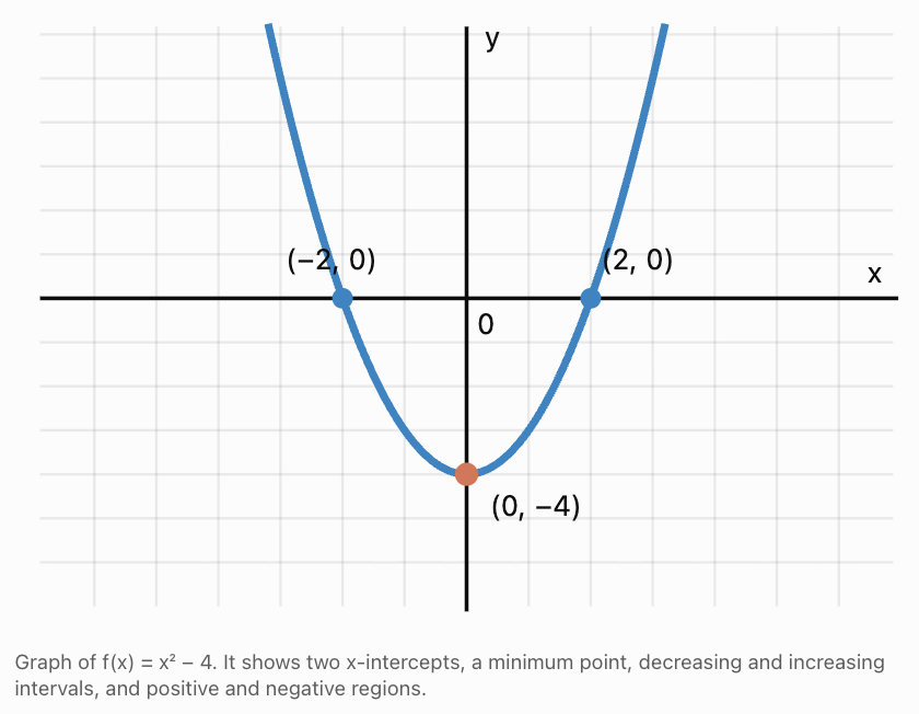
From this graph, we can identify several important features without calculating every possible output.
The graph crosses the x-axis at x = −2 and x = 2. It reaches a minimum at (0, −4). It decreases to the left of the minimum and increases to the right.
These features form the foundation of function analysis.
Intercepts
An intercept is a point where a graph meets one of the coordinate axes.
x-Intercepts
An x-intercept occurs where the output is zero.
Therefore:
f(x) = 0
To find x-intercepts algebraically, solve the equation f(x) = 0.
Worked Example 1: Finding x-Intercepts
Find the x-intercepts of:
f(x) = x² − 5x + 6
Step 1: Set the function equal to zero.
x² − 5x + 6 = 0
Step 2: Factor.
(x − 2)(x − 3) = 0
Step 3: Solve.
x = 2 or x = 3
Answer: x-intercepts (2, 0) and (3, 0).
y-Intercepts
A y-intercept occurs when x = 0.
Therefore, calculate:
f(0)
Worked Example 2: Finding a y-Intercept
For:
f(x) = x² − 5x + 6
Substitute x = 0:
f(0) = 0² − 5(0) + 6
f(0) = 6
Answer: y-intercept (0, 6).
Intercepts of Rational Functions
For a rational function:
f(x) = P(x)/Q(x)
x-intercepts occur where P(x) = 0, provided Q(x) ≠ 0.
The y-intercept is f(0), provided the function is defined at x = 0.
For example:
f(x) = (x − 3)/(x + 2)
x-intercept: (3, 0).
y-intercept: (0, −3/2).
The function is undefined at x = −2.
Interpreting Intercepts
Intercepts often have important practical meanings.
For a height–time graph, an x-intercept may represent the moment an object reaches the ground.
For a profit–production graph, an x-intercept may represent the break-even point.
For a population model, the y-intercept may represent the initial population.
Always interpret intercepts using the units and context of the problem.
Maximum and Minimum Values
An extremum is a maximum or minimum value of a function.
The plural is extrema.
There are two important types.
Local maximum: A point where the function value is greater than or equal to nearby function values.
Local minimum: A point where the function value is less than or equal to nearby function values.
An absolute maximum is the greatest output over the entire domain being considered.
An absolute minimum is the smallest output over that domain.
A local extremum does not necessarily have to be an absolute extremum.
Worked Example 3: Finding the Minimum of a Quadratic Function
Consider:
f(x) = x² − 6x + 5
Since the coefficient of x² is positive, the parabola opens upward.
The minimum occurs at its vertex.
For a quadratic:
f(x) = ax² + bx + c
the vertex x-coordinate is:
x = −b/(2a)
Here:
a = 1, b = −6
Therefore:
x = 6/2 = 3
Substitute:
f(3) = 3² − 6(3) + 5
= 9 − 18 + 5
= −4
Minimum point: (3, −4).
The minimum output is −4.
The function has no absolute maximum because it increases without bound.
Worked Example 4: Finding a Maximum
Consider:
h(t) = −5t² + 30t + 2
This could represent the height of an object above the ground.
The parabola opens downward, so its vertex is a maximum.
t = −30/[2(−5)]
t = 3
Calculate:
h(3) = −5(9) + 30(3) + 2
= −45 + 90 + 2
= 47
Maximum height: 47 m, reached after 3 seconds.
Local Versus Absolute Extrema
A cubic or higher-degree polynomial may have several turning points.
For example:
f(x) = x³ − 3x
has a local maximum at (−1, 2) and a local minimum at (1, −2).
However, the function has no absolute maximum or minimum on the real number line because its outputs extend without bound in both directions.
This distinction is important when interpreting graphs.
Intervals of Increase and Decrease
A function is increasing on an interval when its output becomes larger as x increases.
A function is decreasing on an interval when its output becomes smaller as x increases.
We describe these intervals using x-values, not y-values.
Example: Quadratic Function
Consider:
f(x) = (x − 2)² + 1
The vertex is (2, 1).
The parabola opens upward.
Therefore:
-
The function is decreasing on (−∞, 2).
-
The function is increasing on (2, ∞).
The turning point x = 2 separates the two intervals.
Worked Example 5: Increasing and Decreasing Intervals
Consider:
f(x) = x³ − 3x
This function has a local maximum at x = −1 and a local minimum at x = 1.
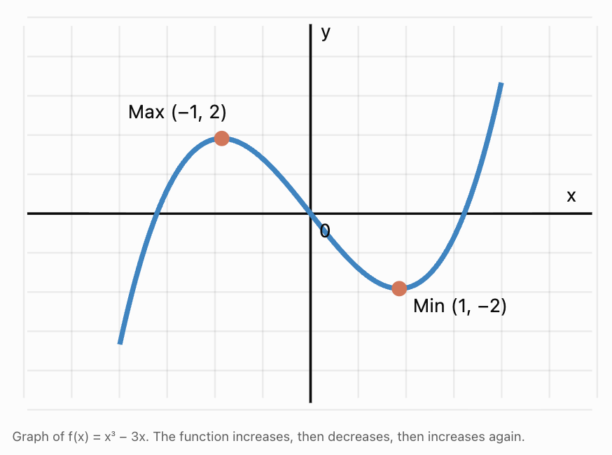
Reading from left to right:
The graph rises until x = −1.
It then falls between x = −1 and x = 1.
After x = 1, it rises again.
Therefore:
|
Interval |
Behaviour |
|---|---|
|
(−∞, −1) |
Increasing |
|
(−1, 1) |
Decreasing |
|
(1, ∞) |
Increasing |
Using a Table to Identify Behaviour
Consider:
f(x) = x² − 4x + 3
|
x |
f(x) |
|---|---|
|
0 |
3 |
|
1 |
0 |
|
2 |
−1 |
|
3 |
0 |
|
4 |
3 |
As x increases from 0 to 2, the outputs decrease.
As x increases from 2 to 4, the outputs increase.
This suggests a minimum at x = 2.
The complete intervals are:
Decreasing: (−∞, 2)
Increasing: (2, ∞)
A table can reveal a pattern, but it does not by itself prove the behaviour across every value in an interval.
Increasing and Decreasing Rational Functions
Consider:
f(x) = 1/x
The function decreases on both:
(−∞, 0) and (0, ∞).
However, it is not decreasing across its entire domain as one interval because x = 0 is excluded and the branches are separated.
Always divide intervals at discontinuities.
End Behaviour
End behaviour describes how a function behaves as x approaches positive infinity or negative infinity.
We are interested in what happens at the far left and far right of a graph.
End Behaviour of Polynomial Functions
The leading term usually determines the end behaviour.
For example:
f(x) = 2x⁴ − 3x² + 1
The leading term is 2x⁴.
Because the degree is even and the leading coefficient is positive, both ends rise.
|
Polynomial type |
As x → −∞ |
As x → +∞ |
|---|---|---|
|
Even degree, positive leading coefficient |
f(x) → +∞ |
f(x) → +∞ |
|
Even degree, negative leading coefficient |
f(x) → −∞ |
f(x) → −∞ |
|
Odd degree, positive leading coefficient |
f(x) → −∞ |
f(x) → +∞ |
|
Odd degree, negative leading coefficient |
f(x) → +∞ |
f(x) → −∞ |
Worked Example 6: Polynomial End Behaviour
Analyze:
f(x) = −3x⁵ + 2x³ − 7
The leading term is −3x⁵.
The degree is odd.
The leading coefficient is negative.
Therefore:
As x → −∞, f(x) → +∞.
As x → +∞, f(x) → −∞.
Interpretation: The graph rises on the left and falls on the right.
End Behaviour of Rational Functions
Rational functions often approach horizontal, oblique, or higher-degree polynomial asymptotes.
Consider:
f(x) = (2x + 1)/(x − 3)
Both numerator and denominator have degree 1.
The horizontal asymptote is the ratio of leading coefficients:
y = 2/1 = 2
Therefore:
As x → −∞, f(x) → 2.
As x → +∞, f(x) → 2.
Worked Example 7: Interpreting an Oblique Asymptote
Consider:
f(x) = (x² + 1)/(x − 2)
Polynomial division gives:
f(x) = x + 2 + 5/(x − 2)
As x becomes very large in magnitude:
5/(x − 2) approaches zero.
Therefore, the graph approaches:
y = x + 2
This is an oblique asymptote.
For large positive x, the graph approaches the line from above.
For large negative x, it approaches the line from below.
Vertical and Horizontal Asymptotes
An asymptote describes a line that a function approaches in a particular limiting situation.
Vertical Asymptotes
Vertical asymptotes occur at certain excluded x-values where function values grow without bound.
Consider:
f(x) = 1/(x − 2)
Vertical asymptote:
x = 2
As x approaches 2 from the left, f(x) approaches negative infinity.
As x approaches 2 from the right, f(x) approaches positive infinity.
Horizontal Asymptotes
Horizontal asymptotes describe behaviour as x approaches positive or negative infinity.
Consider:
f(x) = 3 + 2/x
Horizontal asymptote:
y = 3
As x becomes very large in magnitude, 2/x approaches zero.
Worked Example 8: Identifying Asymptotes
Analyze:
f(x) = (3x + 2)/(x − 4)
Vertical asymptote:
x − 4 = 0
x = 4
Horizontal asymptote:
Both polynomials have degree 1.
Leading coefficient ratio:
3/1 = 3
Therefore:
y = 3
Answer: Vertical asymptote x = 4; horizontal asymptote y = 3.
Positive and Negative Intervals
A function is positive when:
f(x) > 0
Its graph lies above the x-axis.
A function is negative when:
f(x) < 0
Its graph lies below the x-axis.
The points where f(x) = 0 separate positive and negative regions, although the sign does not always change at a zero.
Worked Example 9: Positive and Negative Intervals of a Quadratic
Consider:
f(x) = x² − 5x + 6
Factor:
f(x) = (x − 2)(x − 3)
The zeros are:
x = 2 and x = 3.
These divide the number line into three intervals.
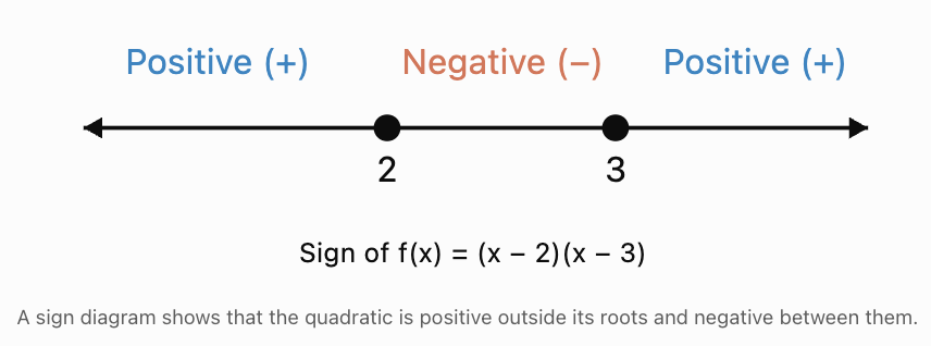
Test each interval.
Interval 1: x less than 2
Choose x = 0.
f(0) = 6
Positive.
Interval 2: 2 less than x less than 3
Choose x = 2.5.
f(2.5) = (0.5)(−0.5) = −0.25
Negative.
Interval 3: x greater than 3
Choose x = 4.
f(4) = (2)(1) = 2
Positive.
Therefore:
Positive on (−∞, 2) ∪ (3, ∞).
Negative on (2, 3).
The function equals zero at x = 2 and x = 3.
Worked Example 10: Sign Analysis of a Rational Function
Consider:
The numerator is zero at x = 1.
The denominator is zero at x = −2.
These values divide the number line into three intervals.
|
Interval |
Test x |
Sign of f(x) |
|---|---|---|
|
x less than −2 |
−3 |
Positive |
|
−2 less than x less than 1 |
0 |
Negative |
|
x greater than 1 |
2 |
Positive |
Therefore:
Positive: (−∞, −2) ∪ (1, ∞).
Negative: (−2, 1).
At x = 1, the function equals zero.
At x = −2, the function is undefined.
Important: A zero and a vertical asymptote can both separate sign intervals, but they have different meanings.
A Complete Method for Analysing Function Behaviour
When presented with an unfamiliar function, use the following process.
-
Identify the function type. Determine whether it is linear, quadratic, polynomial, rational, exponential, or another family.
-
Determine the domain. Identify permitted inputs and any excluded values.
-
Find intercepts. Solve f(x) = 0 and calculate f(0), where defined.
-
Identify extrema. Find maximum and minimum points using algebra, a graph, or calculus where appropriate.
-
Find asymptotes. Check for vertical, horizontal, and oblique asymptotes.
-
Determine intervals of increase and decrease. Identify where the graph rises or falls.
-
Determine positive and negative intervals. Use zeros, discontinuities, and test values.
-
Describe end behaviour. Explain what happens as x approaches positive and negative infinity.
-
Interpret the features. Explain their mathematical or real-world meaning.
Worked Example 11: Complete Analysis of a Quadratic Function
Analyze:
f(x) = −x² + 4x + 5
Step 1: Domain
This is a polynomial function.
Domain: all real numbers.
Step 2: x-Intercepts
Set f(x) = 0:
−x² + 4x + 5 = 0
Multiply by −1:
x² − 4x − 5 = 0
Factor:
(x − 5)(x + 1) = 0
Therefore:
x = 5 or x = −1
x-intercepts: (−1, 0) and (5, 0).
Step 3: y-Intercept
f(0) = 5
y-intercept: (0, 5).
Step 4: Maximum or Minimum
The coefficient of x² is negative, so the parabola opens downward.
Vertex x-coordinate:
x = −4/[2(−1)] = 2
Calculate:
f(2) = −4 + 8 + 5 = 9
Maximum point: (2, 9).
Step 5: Increasing and Decreasing Intervals
Increasing: (−∞, 2).
Decreasing: (2, ∞).
Step 6: Positive and Negative Intervals
The zeros are x = −1 and x = 5.
Because the parabola opens downward:
Positive: (−1, 5).
Negative: (−∞, −1) ∪ (5, ∞).
Step 7: End Behaviour
As x → −∞, f(x) → −∞.
As x → +∞, f(x) → −∞.
Step 8: Range
The maximum output is 9.
Range: (−∞, 9].
Summary
|
Feature |
Result |
|---|---|
|
Domain |
All real numbers |
|
Range |
y ≤ 9 |
|
x-intercepts |
(−1, 0), (5, 0) |
|
y-intercept |
(0, 5) |
|
Maximum |
(2, 9) |
|
Increasing |
(−∞, 2) |
|
Decreasing |
(2, ∞) |
|
Positive |
(−1, 5) |
|
Negative |
x less than −1 or greater than 5 |
|
End behaviour |
Both ends fall |
Worked Example 12: Complete Analysis of a Rational Function
Analyze:
Step 1: Domain
The denominator is zero at x = 2.
Domain: x ≠ 2.
Step 2: Intercepts
x-intercept:
x + 1 = 0
x = −1
Therefore, (−1, 0).
y-intercept:
f(0) = 1/(−2) = −1/2
Therefore, (0, −1/2).
Step 3: Asymptotes
Vertical asymptote:
x = 2
Horizontal asymptote:
Both polynomials have degree 1, with leading coefficient ratio 1.
Therefore:
y = 1
Step 4: Increasing and Decreasing Intervals
Rewrite:
f(x) = 1 + 3/(x − 2)
As x increases on either side of x = 2, the term 3/(x − 2) decreases.
Therefore:
Decreasing: (−∞, 2) and (2, ∞).
There are no increasing intervals.
Step 5: Positive and Negative Intervals
Critical values:
x = −1 and x = 2.
Test the intervals.
For x less than −1, the numerator and denominator are both negative, so f(x) is positive.
For −1 less than x less than 2, the numerator is positive and denominator negative, so f(x) is negative.
For x greater than 2, both are positive, so f(x) is positive.
Therefore:
Positive: (−∞, −1) ∪ (2, ∞).
Negative: (−1, 2).
Step 6: End Behaviour
As x → −∞, f(x) → 1 from below.
As x → +∞, f(x) → 1 from above.
Step 7: Range
Since f(x) = 1 + 3/(x − 2), the function cannot equal 1.
Range: all real numbers except 1.
Summary
|
Feature |
Result |
|---|---|
|
Domain |
x ≠ 2 |
|
Range |
y ≠ 1 |
|
x-intercept |
(−1, 0) |
|
y-intercept |
(0, −1/2) |
|
Vertical asymptote |
x = 2 |
|
Horizontal asymptote |
y = 1 |
|
Increasing |
None |
|
Decreasing |
(−∞, 2), (2, ∞) |
|
Positive |
x less than −1 or greater than 2 |
|
Negative |
−1 less than x less than 2 |
Real-World Applications
Application 1: Maximum Height of a Projectile
A ball is launched upward from a height of 2 metres.
Its height is modelled by:
h(t) = −5t² + 20t + 2
where t is time in seconds.
Maximum height:
t = −20/[2(−5)] = 2 seconds
h(2) = −5(4) + 20(2) + 2
= 22 m
The maximum occurs at (2, 22).
The ball rises for the first 2 seconds and falls after 2 seconds.
The model is physically meaningful only until the ball reaches the ground.
Solving h(t) = 0 gives:
t = 2 + √110/5 ≈ 4.10 seconds.
Therefore:
Increasing during 0 < t < 2.
Decreasing during 2 < t < 4.10.
The function's maximum represents the highest point of the ball's flight.
Application 2: Business Profit
A company's profit is modelled by:
P(x) = −2x² + 80x − 600
where x is the number of units produced and P(x) is measured in dollars.
Find the break-even points.
Set P(x) = 0:
−2x² + 80x − 600 = 0
Divide by −2:
x² − 40x + 300 = 0
Factor:
(x − 10)(x − 30) = 0
Therefore:
x = 10 or x = 30.
The company breaks even at 10 and 30 units.
Find maximum profit.
Vertex x-coordinate:
x = −80/[2(−2)] = 20
P(20) = −2(400) + 80(20) − 600
= −800 + 1600 − 600
= 200
Maximum profit = $200 at 20 units.
Interpret the signs.
Profit is positive for 10 < x < 30.
Profit is negative for x < 10 or x > 30.
For a real production model, only nonnegative whole-number values of x are meaningful.
Application 3: Average Cost
Suppose:
A(x) = 600/x + 15
where A(x) is average cost per item and x is the number of items.
The function is decreasing for x > 0.
As x becomes very large, A(x) approaches 15.
The horizontal asymptote is:
y = 15.
This means average cost approaches $15 per item as production increases.
The mathematical model has a vertical asymptote at x = 0, but the practical domain consists of positive whole-number production quantities.
Application 4: Interpreting a Population Graph
Suppose a population is modelled by:
P(t) = 500 + 200t − 10t²
where t represents years after the start of a study.
The graph initially increases because the linear growth term dominates.
Eventually, the negative quadratic term causes the model to reach a maximum and then decrease.
The maximum occurs at:
t = −200/[2(−10)] = 10
P(10) = 500 + 2000 − 1000
= 1500
The model predicts a maximum population of 1,500 after 10 years.
However, this quadratic model cannot remain realistic indefinitely because it eventually predicts negative population values.
This demonstrates why mathematical features must be interpreted alongside the assumptions and limitations of a model.
Common Mistakes
Mistake 1: Confusing x-Intercepts and y-Intercepts
x-intercepts occur where y = 0.
y-intercepts occur where x = 0.
For example, f(x) = x² − 4 has x-intercepts at (−2, 0) and (2, 0), and a y-intercept at (0, −4).
Mistake 2: Confusing Maximum Values with Maximum Points
For f(x) = −(x − 3)² + 7:
Maximum point: (3, 7).
Maximum value: 7.
The point includes both coordinates, while the value refers only to the output.
Mistake 3: Writing Increasing Intervals Using y-Values
Increasing and decreasing intervals are described using x-values.
For f(x) = (x − 2)²:
Increasing interval: (2, ∞), not (0, ∞).
Mistake 4: Including a Discontinuity in an Interval
For f(x) = 1/x, the function is decreasing on (−∞, 0) and (0, ∞).
It is not appropriate to combine these into one decreasing interval across x = 0.
Mistake 5: Assuming a Horizontal Asymptote Cannot Be Crossed
A graph may cross a horizontal asymptote.
Horizontal asymptotes describe end behaviour rather than forbidden values.
Mistake 6: Confusing Positive Functions with Increasing Functions
A function can be positive while decreasing.
For example, f(x) = 1/x is positive and decreasing for x > 0.
Positive describes the sign of the output.
Increasing describes how the output changes as x increases.
Mistake 7: Forgetting to Test Intervals
Knowing where a function equals zero does not automatically tell us where it is positive or negative.
Use a sign diagram or test values.
Mistake 8: Ignoring Context
A polynomial may be defined for all real numbers mathematically, but a physical model may only be meaningful over a restricted interval.
Always interpret the graph using the situation being modelled.
Key Terms
-
Function: A relationship assigning exactly one output to each input in its domain.
-
Domain: The set of permitted input values.
-
Range: The set of possible output values.
-
x-Intercept: A point where the graph meets the x-axis.
-
y-Intercept: A point where the graph meets the y-axis.
-
Zero or Root: An input value for which f(x) = 0.
-
Extremum: A maximum or minimum value.
-
Local Maximum: A function value greater than or equal to nearby values.
-
Local Minimum: A function value less than or equal to nearby values.
-
Absolute Maximum: The greatest function value over the domain being considered.
-
Absolute Minimum: The smallest function value over the domain being considered.
-
Turning Point: A point where a function changes from increasing to decreasing or vice versa.
-
Increasing Interval: An interval where outputs increase as inputs increase.
-
Decreasing Interval: An interval where outputs decrease as inputs increase.
-
End Behaviour: The behaviour of a function as x approaches positive or negative infinity.
-
Vertical Asymptote: A vertical line approached by a graph as function values grow without bound.
-
Horizontal Asymptote: A horizontal line approached by a graph as x becomes very large in magnitude.
-
Oblique Asymptote: A nonhorizontal straight line approached by a graph at infinity.
-
Positive Interval: An interval where f(x) > 0.
-
Negative Interval: An interval where f(x) < 0.
-
Sign Diagram: A representation showing where a function is positive, negative, zero, or undefined.
-
Critical Value: An input at which a derivative is zero or undefined, when the function itself is defined; such values are candidates for extrema.
-
Mathematical Model: A function or equation representing a real-world relationship.
Key Takeaways
-
Intercepts identify where a graph meets the coordinate axes.
-
Extrema identify maximum and minimum values.
-
Local extrema describe nearby behaviour, while absolute extrema describe the entire domain being considered.
-
Increasing intervals show where outputs rise as x increases.
-
Decreasing intervals show where outputs fall as x increases.
-
End behaviour describes what happens as x approaches positive or negative infinity.
-
Vertical asymptotes describe unbounded behaviour near certain excluded inputs.
-
Horizontal and oblique asymptotes describe long-term graph behaviour.
-
A function is positive above the x-axis and negative below it.
-
Zeros and discontinuities help divide a graph into sign intervals.
-
Positive and increasing are different mathematical properties.
-
Graph features can represent important events such as maximum height, break-even points, and changing costs.
-
A complete function analysis combines algebraic calculations, graphical interpretation, and contextual reasoning.
Check Your Understanding
Question 1: Intercepts
Find the x- and y-intercepts of:
f(x) = x² − 7x + 10
Question 2: Extrema
Find the vertex and determine whether it is a maximum or minimum:
f(x) = −2x² + 8x + 3
Question 3: Increasing and Decreasing Intervals
For:
f(x) = (x + 3)² − 2
Determine the intervals where the function is increasing and decreasing.
Question 4: End Behaviour
Describe the end behaviour of:
f(x) = −4x⁶ + 3x³ − 2
Question 5: Asymptotes
Find the vertical and horizontal asymptotes of:
f(x) = (2x + 5)/(x − 3)
Question 6: Positive and Negative Intervals
Determine where the following function is positive and negative:
f(x) = (x − 1)(x − 4)
Question 7: Rational Function Sign Analysis
Determine where:
f(x) = (x + 2)/(x − 3)
is positive, negative, zero, and undefined.
Question 8: Complete Function Analysis
Analyze:
f(x) = −x² + 6x − 5
Find:
a) Domain and range.
b) x- and y-intercepts.
c) Maximum or minimum point.
d) Increasing and decreasing intervals.
e) Positive and negative intervals.
f) End behaviour.
Question 9: Real-World Application
A ball's height is given by:
h(t) = −5t² + 25t + 1
where t is measured in seconds and h is measured in metres.
a) Find the initial height.
b) Determine when the ball reaches maximum height.
c) Calculate the maximum height.
d) Find approximately when the ball reaches the ground.
e) Explain the meaning of the increasing and decreasing intervals.
Question 10: Challenge
Analyze:
f(x) = (x − 2)/(x + 1)
Find:
a) Domain.
b) Range.
c) x- and y-intercepts.
d) Vertical and horizontal asymptotes.
e) Increasing or decreasing intervals.
f) Positive and negative intervals.
g) End behaviour.
Fully Worked Answers
Answer 1: Intercepts
Given:
f(x) = x² − 7x + 10
x-intercepts:
Set f(x) = 0:
x² − 7x + 10 = 0
Factor:
(x − 2)(x − 5) = 0
Therefore:
x = 2 or x = 5
x-intercepts: (2, 0) and (5, 0).
y-intercept:
f(0) = 10
y-intercept: (0, 10).
Answer 2: Extrema
Given:
f(x) = −2x² + 8x + 3
The coefficient of x² is negative, so the parabola opens downward.
Vertex x-coordinate:
x = −8/[2(−2)] = 2
Substitute:
f(2) = −2(4) + 8(2) + 3
= −8 + 16 + 3
= 11
Answer: Maximum point (2, 11).
Answer 3: Increasing and Decreasing
Given:
f(x) = (x + 3)² − 2
The vertex is (−3, −2).
The parabola opens upward.
Therefore:
Decreasing: (−∞, −3).
Increasing: (−3, ∞).
Answer 4: End Behaviour
Given:
f(x) = −4x⁶ + 3x³ − 2
The leading term is −4x⁶.
The degree is even and the leading coefficient is negative.
Therefore:
As x → −∞, f(x) → −∞.
As x → +∞, f(x) → −∞.
Answer: Both ends of the graph fall.
Answer 5: Asymptotes
Given:
f(x) = (2x + 5)/(x − 3)
Vertical asymptote:
x − 3 = 0
x = 3
Horizontal asymptote:
Both polynomials have degree 1.
Leading coefficient ratio:
2/1 = 2
Therefore:
y = 2.
Answer: x = 3 and y = 2.
Answer 6: Positive and Negative Intervals
Given:
f(x) = (x − 1)(x − 4)
Zeros:
x = 1 and x = 4.
Test intervals.
For x less than 1, both factors are negative, so their product is positive.
For 1 less than x less than 4, the first factor is positive and the second negative, so the product is negative.
For x greater than 4, both factors are positive, so their product is positive.
Positive: (−∞, 1) ∪ (4, ∞).
Negative: (1, 4).
The function equals zero at x = 1 and x = 4.
Answer 7: Rational Function Sign Analysis
Given:
f(x) = (x + 2)/(x − 3)
Numerator zero:
x + 2 = 0
x = −2
Denominator zero:
x − 3 = 0
x = 3
Critical boundaries for sign analysis:
−2 and 3.
For x less than −2, both numerator and denominator are negative, so f(x) is positive.
For −2 less than x less than 3, the numerator is positive and denominator negative, so f(x) is negative.
For x greater than 3, both are positive, so f(x) is positive.
Positive: (−∞, −2) ∪ (3, ∞).
Negative: (−2, 3).
Zero: x = −2.
Undefined: x = 3.
Answer 8: Complete Function Analysis
Given:
f(x) = −x² + 6x − 5
a) Domain and range
The domain is all real numbers.
Find the vertex:
x = −6/[2(−1)] = 3
f(3) = −9 + 18 − 5 = 4
The maximum output is 4.
Range: (−∞, 4].
b) Intercepts
Set f(x) = 0:
−x² + 6x − 5 = 0
Multiply by −1:
x² − 6x + 5 = 0
Factor:
(x − 1)(x − 5) = 0
x-intercepts: (1, 0) and (5, 0).
y-intercept:
f(0) = −5
Therefore, (0, −5).
c) Maximum or minimum
Maximum point: (3, 4).
d) Increasing and decreasing
Increasing: (−∞, 3).
Decreasing: (3, ∞).
e) Positive and negative
The parabola opens downward and has roots at 1 and 5.
Positive: (1, 5).
Negative: (−∞, 1) ∪ (5, ∞).
f) End behaviour
As x → −∞, f(x) → −∞.
As x → +∞, f(x) → −∞.
Answer 9: Projectile Motion
Given:
h(t) = −5t² + 25t + 1
a) Initial height
h(0) = 1
Initial height = 1 m.
b) Time of maximum height
t = −25/[2(−5)]
t = 2.5 seconds.
c) Maximum height
h(2.5) = −5(2.5²) + 25(2.5) + 1
= −31.25 + 62.5 + 1
= 32.25 m.
d) Time when the ball reaches the ground
Set h(t) = 0:
−5t² + 25t + 1 = 0
Multiply by −1:
5t² − 25t − 1 = 0
Using the quadratic formula:
The positive root is approximately:
t ≈ 5.04 seconds.
The negative root is not meaningful for time after launch.
e) Increasing and decreasing intervals
The ball rises from t = 0 to t = 2.5 seconds.
It falls from t = 2.5 seconds until it reaches the ground at approximately 5.04 seconds.
Therefore:
Increasing: (0, 2.5).
Decreasing: (2.5, 5.04), approximately.
Answer 10: Challenge
Given:
f(x) = (x − 2)/(x + 1)
a) Domain
The denominator is zero at x = −1.
Domain: x ≠ −1.
b) Range
Rewrite:
f(x) = 1 − 3/(x + 1)
The function cannot equal 1 because −3/(x + 1) cannot equal zero.
Range: y ≠ 1.
c) Intercepts
x-intercept:
x − 2 = 0
x = 2
Therefore, (2, 0).
y-intercept:
f(0) = −2
Therefore, (0, −2).
d) Asymptotes
Vertical asymptote: x = −1.
Horizontal asymptote: y = 1.
e) Increasing and decreasing intervals
Rewrite:
f(x) = 1 − 3/(x + 1)
As x increases on either side of x = −1, the function increases.
Increasing:
(−∞, −1) and (−1, ∞).
There are no decreasing intervals.
f) Positive and negative intervals
Critical boundaries:
x = −1 and x = 2.
For x less than −1, numerator and denominator are negative, so the function is positive.
For −1 less than x less than 2, the numerator is negative and denominator positive, so the function is negative.
For x greater than 2, both are positive, so the function is positive.
Positive:
(−∞, −1) ∪ (2, ∞).
Negative:
(−1, 2).
g) End behaviour
As x → −∞, f(x) approaches 1 from above.
As x → +∞, f(x) approaches 1 from below.
Near the vertical asymptote:
As x approaches −1 from the left, f(x) approaches positive infinity.
As x approaches −1 from the right, f(x) approaches negative infinity.
This completes Function Features and Behaviour, covering all five learning targets with graphical illustrations, algebraic analysis, real-world applications, common mistakes, key terms, key takeaways, and fully worked practice questions.
3. Function Transformations Review
Learning outcomes
- I can apply transformations to polynomial functions.
- I can apply transformations to rational functions.
- I can predict graph changes from equations.
- I can write transformed function equations.
- I can sketch transformed graphs accurately.
Introduction
Functions are used to describe patterns, relationships, and changes in the world around us. Once we understand the graph of a basic function, we can create many new graphs by shifting, reflecting, stretching, or compressing it.
These changes are called function transformations.
For example, the basic quadratic function:
f(x) = x²
produces a parabola with its vertex at the origin.
By changing its equation to:
g(x) = (x − 3)² + 2
we move the parabola 3 units to the right and 2 units upward.
The shape remains the same, but its position changes.
Function transformations are especially useful because they allow us to predict the shape and location of a graph without plotting large numbers of points.
The same transformation principles apply to polynomial functions, rational functions, exponential functions, and many other families.
In this lesson, we will review how transformations affect polynomial and rational functions, predict graph changes from equations, write transformed equations, and sketch graphs using key features.
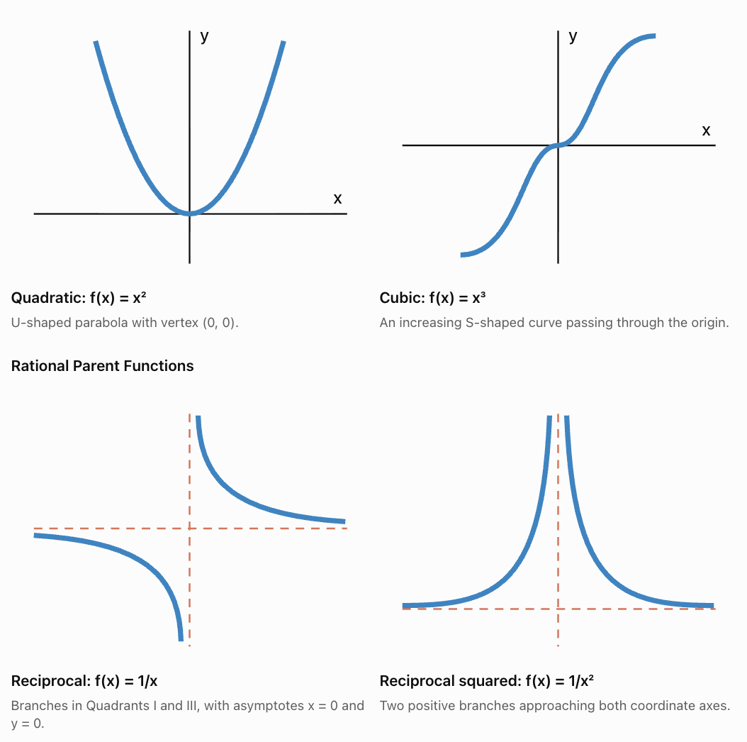
Understanding Parent Functions
A parent function is a basic function from which other related functions can be produced through transformations.
Common parent functions include:
|
Function family |
Parent function |
Graph shape |
|---|---|---|
|
Linear |
f(x) = x |
Straight line |
|
Quadratic |
f(x) = x² |
Parabola |
|
Cubic |
f(x) = x³ |
S-shaped curve |
|
Absolute value |
f(x) = |x| |
V-shaped graph |
|
Reciprocal |
f(x) = 1/x |
Two hyperbola branches |
|
Reciprocal squared |
f(x) = 1/x² |
Two branches above the x-axis |
In this lesson, we focus mainly on polynomial and rational parent functions.
Polynomial Parent Functions
The General Transformation Equation
Many transformed functions can be written as:
where:
-
a controls vertical stretching, compression, and reflection in the x-axis.
-
b controls horizontal stretching, compression, and reflection in the y-axis.
-
h controls horizontal translation.
-
k controls vertical translation.
These parameters affect the graph in predictable ways.
|
Transformation |
Equation |
Effect |
|---|---|---|
|
Vertical translation |
f(x) + k |
Up k units if k > 0 |
|
Vertical translation |
f(x) − k |
Down k units if k > 0 |
|
Horizontal translation |
f(x − h) |
Right h units if h > 0 |
|
Horizontal translation |
f(x + h) |
Left h units if h > 0 |
|
Vertical stretch |
af(x), |a| > 1 |
Outputs move farther from x-axis |
|
Vertical compression |
af(x), 0 < |a| < 1 |
Outputs move closer to x-axis |
|
Reflection in x-axis |
−f(x) |
Outputs change sign |
|
Reflection in y-axis |
f(−x) |
Inputs change sign |
|
Horizontal compression |
f(bx), |b| > 1 |
x-coordinates divided by |b| |
|
Horizontal stretch |
f(bx), 0 < |b| < 1 |
x-coordinates multiplied by 1/|b| |
Important: Horizontal transformations work in the opposite direction from what the sign inside the brackets might initially suggest.
For example:
f(x − 4) moves the graph right 4 units, not left.
Vertical Translations
A vertical translation moves every point on a graph up or down.
If:
g(x) = f(x) + k
then every output increases by k.
The point (x, y) becomes:
(x, y + k)
Worked Example 1: Vertical Translation of a Polynomial
Consider:
f(x) = x²
Translate the graph upward 5 units.
The new equation is:
g(x) = x² + 5
The vertex moves from (0, 0) to (0, 5).
The domain remains all real numbers.
The range changes from y ≥ 0 to y ≥ 5.
Worked Example 2: Vertical Translation of a Rational Function
Consider:
f(x) = 1/x
Translate the graph downward 3 units.
The new equation is:
g(x) = 1/x − 3
The vertical asymptote remains:
x = 0
The horizontal asymptote moves from y = 0 to:
y = −3
The domain remains x ≠ 0.
The range becomes y ≠ −3.
Horizontal Translations
A horizontal translation moves a graph left or right.
If:
g(x) = f(x − h)
the graph moves right h units when h is positive.
If:
g(x) = f(x + h)
the graph moves left h units when h is positive.
Worked Example 3: Horizontal Translation of a Quadratic
Consider:
f(x) = x²
Translate the graph right 4 units.
The new equation is:
g(x) = (x − 4)²
The vertex moves from (0, 0) to (4, 0).
The axis of symmetry becomes:
x = 4
Worked Example 4: Horizontal Translation of a Rational Function
Consider:
f(x) = 1/x
Translate the graph left 2 units.
The new equation is:
g(x) = 1/(x + 2)
The vertical asymptote moves from x = 0 to:
x = −2
The horizontal asymptote remains y = 0.
The domain becomes x ≠ −2.
Reflections
Reflections produce mirror images of graphs.
Reflection in the x-Axis
To reflect a function in the x-axis:
g(x) = −f(x)
Every output changes sign.
A point (x, y) becomes:
(x, −y)
Worked Example 5: Reflecting a Quadratic
Original:
f(x) = x²
Reflected:
g(x) = −x²
The parabola changes from opening upward to opening downward.
The vertex remains at (0, 0).
The range changes from y ≥ 0 to y ≤ 0.
Reflection in the y-Axis
To reflect a function in the y-axis:
g(x) = f(−x)
A point (x, y) becomes:
(−x, y)
Worked Example 6: Reflecting a Cubic
Original:
f(x) = x³
Reflected:
g(x) = (−x)³
Therefore:
g(x) = −x³
The graph changes from increasing to decreasing.
Symmetry and Reflections
Some functions remain unchanged under certain reflections.
For example:
f(x) = x²
Then:
f(−x) = (−x)² = x²
The graph is symmetric about the y-axis.
Such functions are called even functions.
For:
f(x) = x³
f(−x) = −x³ = −f(x)
This function is symmetric about the origin and is called an odd function.
These symmetry properties can make some transformations appear to have the same effect.
Vertical Stretches and Compressions
A vertical stretch or compression changes the distance of each point from the x-axis.
For:
g(x) = af(x)
the output values are multiplied by a.
-
If |a| > 1, the graph is stretched vertically.
-
If 0 < |a| < 1, the graph is compressed vertically.
-
If a < 0, the graph is also reflected in the x-axis.
Worked Example 7: Stretching a Quadratic
Original function:
f(x) = x²
Apply a vertical stretch by a factor of 3.
New equation:
g(x) = 3x²
Compare the outputs:
|
x |
f(x) = x² |
g(x) = 3x² |
|---|---|---|
|
−2 |
4 |
12 |
|
−1 |
1 |
3 |
|
0 |
0 |
0 |
|
1 |
1 |
3 |
|
2 |
4 |
12 |
The transformed parabola appears narrower because its outputs increase more quickly as x moves away from zero.
The vertex remains at (0, 0).
Worked Example 8: Compressing a Rational Function
Original:
f(x) = 1/x
Apply a vertical compression by a factor of 1/2.
New equation:
g(x) = 1/(2x)
Every output is half its original value.
For example:
f(2) = 1/2
g(2) = 1/4
The asymptotes remain x = 0 and y = 0.
The branches move closer to the x-axis for corresponding x-values.
Horizontal Stretches and Compressions
Horizontal transformations change the x-coordinates of points.
For:
g(x) = f(bx)
the x-coordinates are divided by b, provided b ≠ 0.
If b = 2, the graph is compressed horizontally by a factor of 1/2.
If b = 1/3, the graph is stretched horizontally by a factor of 3.
Worked Example 9: Horizontal Compression of a Cubic
Original:
f(x) = x³
Apply a horizontal compression by a factor of 1/2.
New equation:
g(x) = f(2x)
Therefore:
g(x) = (2x)³ = 8x³
The original point (2, 8) moves to (1, 8).
Although the equation resembles a vertical stretch by a factor of 8, the specified transformation was a horizontal compression.
Important: Different transformations can sometimes produce the same final equation, particularly for power functions.
Worked Example 10: Horizontal Stretch of a Rational Function
Original:
f(x) = 1/(x − 1)
Apply a horizontal stretch by a factor of 2.
New equation:
g(x) = f(x/2)
Substitute x/2 for x:
Multiply numerator and denominator by 2:
The original vertical asymptote x = 1 moves to x = 2.
The horizontal asymptote remains y = 0.
Combining Transformations
Most transformed functions involve more than one transformation.
The general equation is:
g(x) = af(b(x − h)) + k
A point (u, v) on the original graph transforms to:
This coordinate rule is particularly useful for accurate sketching.
Worked Example 11: Transforming a Quadratic Function
Starting with:
f(x) = x²
Apply the following transformations:
-
Reflect in the x-axis.
-
Stretch vertically by a factor of 2.
-
Translate right 3 units.
-
Translate upward 4 units.
Step 1: Reflection and vertical stretch.
−2x²
Step 2: Horizontal translation.
−2(x − 3)²
Step 3: Vertical translation.
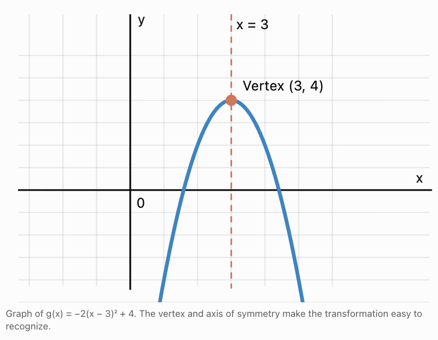
The vertex is (3, 4).
The parabola opens downward.
The maximum value is 4.
The axis of symmetry is x = 3.
The domain is all real numbers.
The range is y ≤ 4.
Sketching the Transformed Quadratic
Worked Example 12: Transforming a Rational Function
Starting with:
f(x) = 1/x
Apply the following transformations:
-
Reflect in the x-axis.
-
Stretch vertically by a factor of 3.
-
Translate right 2 units.
-
Translate upward 1 unit.
The resulting equation is:
Vertical asymptote:
x = 2
Horizontal asymptote:
y = 1
Domain:
x ≠ 2
Range:
y ≠ 1
x-intercept:
Set g(x) = 0:
−3/(x − 2) + 1 = 0
3/(x − 2) = 1
x − 2 = 3
x = 5
Therefore, (5, 0).
y-intercept:
g(0) = −3/(−2) + 1
= 3/2 + 1
= 5/2
Therefore, (0, 2.5).
The negative coefficient reverses the orientation of the reciprocal branches. For x less than 2, the graph lies above y = 1. For x greater than 2, it lies below y = 1.
Predicting Graph Changes from Equations
One of the most useful transformation skills is identifying graph changes without plotting points.
Worked Example 13: Interpreting a Polynomial Equation
Consider:
g(x) = 4(x + 2)² − 3
Compare this with:
f(x) = x²
We can identify:
-
A vertical stretch by a factor of 4.
-
A translation left 2 units.
-
A translation down 3 units.
-
No reflection.
The vertex is (−2, −3).
The parabola opens upward.
The range is y ≥ −3.
Worked Example 14: Interpreting a Rational Equation
Consider:
g(x) = 2/(x + 4) − 5
Compare with:
f(x) = 1/x
We can identify:
-
A vertical stretch by a factor of 2.
-
A translation left 4 units.
-
A translation down 5 units.
The vertical asymptote is x = −4.
The horizontal asymptote is y = −5.
The domain excludes x = −4.
The range excludes y = −5.
Worked Example 15: Interpreting a Horizontal Reflection
Consider:
g(x) = (−x + 3)³
Rewrite:
g(x) = [−(x − 3)]³
Starting with f(x) = x³, this represents a reflection in the y-axis followed by a translation right 3 units.
Because the cubic parent function is odd:
g(x) = −(x − 3)³
Therefore, it can also be described as a reflection in the x-axis followed by a translation right 3 units.
The inflection point is (3, 0).
This example demonstrates that the same transformed graph can sometimes be produced by different sequences of transformations.
Writing Equations from Graph Features
We can reverse the transformation process.
Instead of starting with an equation and identifying changes, we use the graph's features to construct an equation.
Worked Example 16: Writing a Quadratic Equation
A parabola has:
-
Vertex (4, −2).
-
Opens upward.
-
Passes through (5, 1).
Write its equation.
Step 1: Use vertex form.
g(x) = a(x − h)² + k
Substitute the vertex:
g(x) = a(x − 4)² − 2
Step 2: Substitute the known point.
1 = a(5 − 4)² − 2
1 = a − 2
a = 3
Final equation:
Worked Example 17: Writing a Rational Function
A transformed reciprocal graph has:
-
Vertical asymptote x = 3.
-
Horizontal asymptote y = −2.
-
Passes through (4, 1).
Write its equation.
Step 1: Use transformed reciprocal form.
g(x) = a/(x − h) + k
Step 2: Substitute the asymptotes.
h = 3 and k = −2.
Therefore:
g(x) = a/(x − 3) − 2
Step 3: Substitute the known point.
1 = a/(4 − 3) − 2
1 = a − 2
a = 3
Final equation:
This is a vertical stretch by a factor of 3, followed by a translation right 3 units and down 2 units.
Sketching Transformed Graphs Accurately
A good sketch should show the function's defining features rather than rely on many randomly selected points.
Sketching Polynomial Transformations
For a quadratic function:
g(x) = a(x − h)² + k
-
Identify the vertex (h, k).
-
Determine whether the parabola opens upward or downward.
-
Use |a| to determine its vertical stretch or compression.
-
Draw the axis of symmetry x = h.
-
Plot points on both sides of the vertex.
-
Connect the points with a smooth curve.
Worked Example 18: Sketching a Transformed Quadratic
Sketch:
g(x) = 2(x + 1)² − 3
The vertex is (−1, −3).
The parabola opens upward.
It is stretched vertically by a factor of 2.
The axis of symmetry is x = −1.
Calculate points:
|
x |
g(x) |
|---|---|
|
−3 |
5 |
|
−2 |
−1 |
|
−1 |
−3 |
|
0 |
−1 |
|
1 |
5 |
Plot these points and connect them with a smooth U-shaped curve.
Sketching Rational Transformations
For a transformed reciprocal function:
g(x) = a/(x − h) + k
-
Identify the vertical asymptote x = h.
-
Identify the horizontal asymptote y = k.
-
Draw both asymptotes as dashed lines.
-
Determine the sign of a.
-
Plot points on both sides of the vertical asymptote.
-
Sketch the branches approaching the asymptotes.
For a > 0, the branches lie in the upper-right and lower-left regions relative to the asymptote intersection (h, k).
For a < 0, the branches lie in the upper-left and lower-right regions.
Worked Example 19: Sketching a Transformed Rational Function
Sketch:
g(x) = 2/(x − 1) + 3
Step 1: Identify asymptotes.
Vertical asymptote: x = 1.
Horizontal asymptote: y = 3.
Step 2: Determine orientation.
The coefficient 2 is positive.
The right branch lies above y = 3.
The left branch lies below y = 3.
Step 3: Calculate points.
|
x |
g(x) |
|---|---|
|
−1 |
2 |
|
0 |
1 |
|
0.5 |
−1 |
|
1.5 |
7 |
|
2 |
5 |
|
3 |
4 |
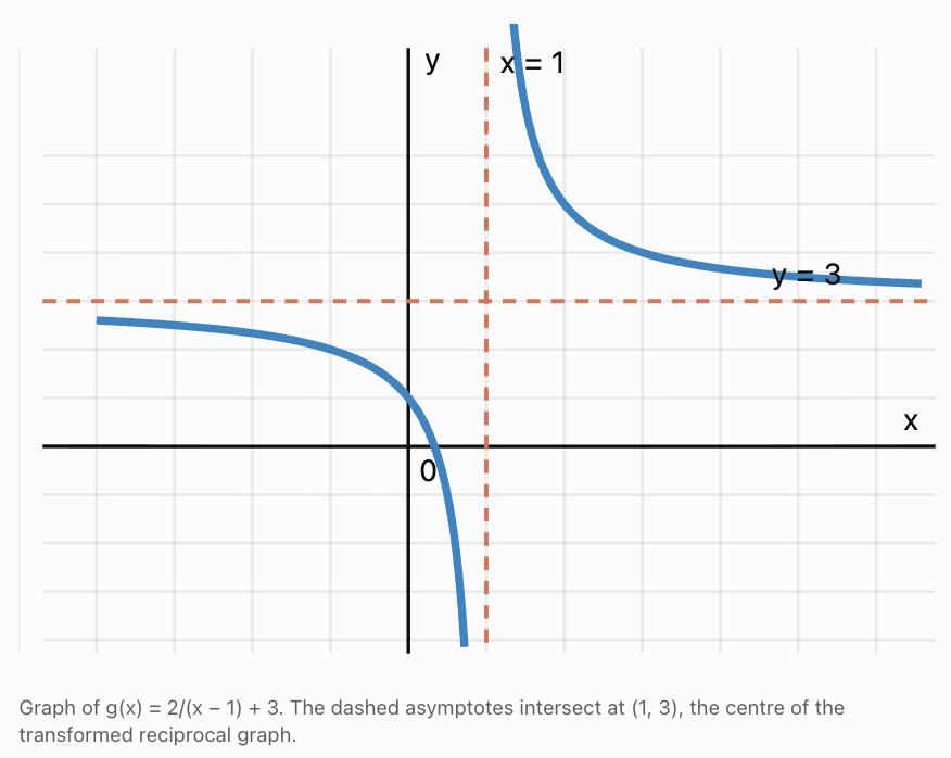
How Transformations Affect Domain, Range, and Asymptotes
Transformations can change more than the appearance of a graph.
They may also change the domain, range, intercepts, extrema, and asymptotes.
Polynomial Functions
For:
g(x) = a(x − h)² + k
with a ≠ 0:
-
Domain: all real numbers.
-
Vertex: (h, k).
-
Axis of symmetry: x = h.
-
Range: y ≥ k if a > 0.
-
Range: y ≤ k if a < 0.
Rational Functions
For:
g(x) = a/(x − h) + k
with a ≠ 0:
-
Domain: x ≠ h.
-
Range: y ≠ k.
-
Vertical asymptote: x = h.
-
Horizontal asymptote: y = k.
These formulas allow us to predict major graph features immediately.
Real-World Applications
Application 1: Projectile Motion
A ball's height is modelled by:
h(t) = −5(t − 3)² + 47
This is a transformed quadratic function.
Compared with f(t) = t², it has been:
-
Reflected in the horizontal axis.
-
Stretched vertically by a factor of 5.
-
Translated right 3 units.
-
Translated upward 47 units.
The vertex is (3, 47).
Interpretation: The ball reaches a maximum height of 47 metres after 3 seconds.
The negative coefficient represents the downward curvature caused by gravity.
The physical model is relevant only over the time interval during which the ball is in flight.
Application 2: Average Production Cost
A company models its average cost per item using:
A(x) = 500/x + 20
This is a transformed reciprocal function.
Compared with f(x) = 1/x:
-
It has been stretched vertically by a factor of 500.
-
It has been translated upward 20 units.
The horizontal asymptote is y = 20.
Interpretation: As production increases, average cost approaches $20 per item.
The vertical asymptote is x = 0, but the practical domain is positive whole-number production quantities.
Application 3: Modelling a Parabolic Arch
An arch is modelled by:
h(x) = −0.25(x − 4)² + 6
where h is height in metres and x is horizontal distance.
The vertex is (4, 6).
The arch reaches a maximum height of 6 metres at x = 4.
To find where it meets ground level, set h(x) = 0:
−0.25(x − 4)² + 6 = 0
0.25(x − 4)² = 6
(x − 4)² = 24
x = 4 ± √24
Approximately:
x ≈ −0.90 and x ≈ 8.90
The arch spans approximately 9.80 metres between its ground-level intercepts.
Application 4: Temperature Adjustment
Suppose a temperature model is:
T(t) = 15 + 10 sin(t)
If a new environment is consistently 5 degrees warmer, the transformed model becomes:
T₂(t) = T(t) + 5
Therefore:
T₂(t) = 20 + 10 sin(t)
This is a vertical translation upward by 5 units.
The maximum and minimum temperatures both increase by 5, while the timing of those extrema remains unchanged.
This demonstrates that transformation principles apply beyond polynomial and rational functions.
Common Mistakes
Mistake 1: Reversing Horizontal Translations
Incorrect: f(x − 3) moves left 3 units.
Correct: f(x − 3) moves right 3 units.
Mistake 2: Confusing Vertical and Horizontal Stretching
The expression 3f(x) represents a vertical stretch by a factor of 3.
The expression f(3x) represents a horizontal compression by a factor of 1/3.
Mistake 3: Forgetting Reflections
A negative coefficient outside the function reflects the graph in the x-axis.
A negative multiplier on the input reflects it in the y-axis.
Mistake 4: Incorrectly Transforming Rational Asymptotes
For g(x) = 1/(x − 4) + 2:
The vertical asymptote is x = 4, not x = −4.
The horizontal asymptote is y = 2, not y = −2.
Mistake 5: Applying Only One Transformation
For g(x) = −3(x + 2)² + 5, the graph is reflected, stretched, shifted left, and shifted upward.
All transformations must be considered.
Mistake 6: Ignoring Domain Restrictions
For rational functions, excluded values must be preserved.
A transformation may move a vertical asymptote or hole to a new location.
Mistake 7: Sketching Without Key Features
For a quadratic, identify the vertex and axis of symmetry first.
For a reciprocal function, identify the asymptotes and branch orientation first.
Mistake 8: Assuming Transformations Always Change the Graph Uniquely
Some transformations produce identical results because of symmetry or algebraic identities.
For example, reflecting y = x² in the y-axis does not change its graph.
Key Terms
-
Parent Function: A basic function used as the starting point for transformations.
-
Transformation: A change in the position, orientation, or scale of a graph.
-
Translation: A shift of a graph without changing its shape.
-
Vertical Translation: Moving a graph upward or downward.
-
Horizontal Translation: Moving a graph left or right.
-
Reflection: Producing a mirror image of a graph across a line.
-
Vertical Stretch: Multiplying outputs by a factor greater than 1 in magnitude.
-
Vertical Compression: Multiplying outputs by a positive factor less than 1.
-
Horizontal Stretch: Increasing horizontal distances by a scale factor.
-
Horizontal Compression: Decreasing horizontal distances by a scale factor.
-
Vertex: The turning point of a parabola.
-
Axis of Symmetry: A line dividing a graph into mirror-image halves.
-
Asymptote: A line that a graph approaches in a particular limiting situation.
-
Vertical Asymptote: A vertical line approached by a graph as outputs become unbounded.
-
Horizontal Asymptote: A horizontal line approached as x tends toward infinity or negative infinity.
-
Domain: The set of permitted input values.
-
Range: The set of possible output values.
-
Even Function: A function satisfying f(−x) = f(x).
-
Odd Function: A function satisfying f(−x) = −f(x).
-
Transformed Equation: An equation produced by applying transformations to a parent function.
Key Takeaways
-
Function transformations allow us to predict new graphs from known parent functions.
-
Adding a constant outside a function moves its graph vertically.
-
Changing the input to x − h moves a graph right h units.
-
Multiplying a function by a negative number reflects it in the x-axis.
-
Replacing x with −x reflects a graph in the y-axis.
-
Vertical stretches and compressions multiply the output values.
-
Horizontal stretches and compressions change the input scale.
-
The general transformation form is g(x) = af(b(x − h)) + k.
-
For a transformed quadratic, the vertex is a key feature for sketching.
-
For a transformed reciprocal function, the asymptotes are key features for sketching.
-
Transformations can change intercepts, extrema, domain restrictions, ranges, and asymptotes.
-
The same transformation rules apply to polynomial, rational, and many other function families.
-
Accurate sketches should include key coordinates, appropriate symmetry, and asymptotes where necessary.
Check Your Understanding
Question 1: Vertical and Horizontal Translations
Starting with f(x) = x², write the equation after translating:
a) Right 4 units.
b) Left 2 units and up 5 units.
c) Right 3 units and down 6 units.
Question 2: Reflections
Starting with f(x) = x³, write the equation after:
a) Reflection in the x-axis.
b) Reflection in the y-axis.
c) Reflection in both axes.
Question 3: Vertical Stretches and Compressions
Starting with f(x) = x², write the equation after:
a) A vertical stretch by a factor of 4.
b) A vertical compression by a factor of 1/3.
c) Reflection in the x-axis followed by a vertical stretch by a factor of 2.
Question 4: Interpreting a Transformed Quadratic
Consider:
g(x) = −3(x − 2)² + 7
Identify:
a) Parent function.
b) Transformations.
c) Vertex.
d) Axis of symmetry.
e) Domain and range.
Question 5: Transforming a Rational Function
Starting with f(x) = 1/x, apply:
-
Translation right 5 units.
-
Translation downward 2 units.
-
Vertical stretch by a factor of 3.
Write the equation and identify its asymptotes.
Question 6: Writing an Equation from a Vertex
A parabola has vertex (−3, 4), opens upward, and passes through (−2, 6).
Write its equation in vertex form.
Question 7: Writing a Rational Function
A reciprocal graph has:
-
Vertical asymptote x = −2.
-
Horizontal asymptote y = 4.
-
Passes through (−1, 7).
Find its equation.
Question 8: Sketching a Transformed Quadratic
Sketch:
g(x) = (x − 1)² − 4
Identify the vertex, axis of symmetry, intercepts, and range.
Question 9: Sketching a Transformed Rational Function
Sketch:
g(x) = −2/(x + 1) + 3
Identify the domain, range, asymptotes, intercepts, and branch orientation.
Question 10: Challenge — Combined Transformations
Starting with:
f(x) = x³
Apply the following transformations:
-
Reflect in the x-axis.
-
Compress horizontally by a factor of 1/2.
-
Translate right 2 units.
-
Translate upward 5 units.
Write the final equation and determine the transformed location of the parent function's origin.
Fully Worked Answers
Answer 1: Translations
a) Right 4 units:
g(x) = (x − 4)²
b) Left 2 and up 5:
g(x) = (x + 2)² + 5
c) Right 3 and down 6:
g(x) = (x − 3)² − 6
Answer 2: Reflections
Original:
f(x) = x³
a) Reflection in x-axis:
g(x) = −x³
b) Reflection in y-axis:
g(x) = (−x)³ = −x³
c) Reflection in both axes:
g(x) = −(−x)³ = x³
The original graph is recovered because the two reflections cancel for this odd function.
Answer 3: Vertical Scaling
a) Vertical stretch by 4:
g(x) = 4x²
b) Vertical compression by 1/3:
g(x) = (1/3)x²
c) Reflection and vertical stretch by 2:
g(x) = −2x²
Answer 4: Transformed Quadratic
Given:
g(x) = −3(x − 2)² + 7
a) Parent function:
f(x) = x²
b) Transformations:
Reflection in x-axis, vertical stretch by factor 3, translation right 2, and translation up 7.
c) Vertex:
(2, 7)
d) Axis of symmetry:
x = 2
e) Domain and range:
Domain: all real numbers.
Range: y ≤ 7.
Answer 5: Rational Transformation
Original:
f(x) = 1/x
Right 5 units:
1/(x − 5)
Vertical stretch by 3:
3/(x − 5)
Down 2 units:
Vertical asymptote:
x = 5
Horizontal asymptote:
y = −2
Answer 6: Quadratic Equation from Vertex
Vertex:
(−3, 4)
Use vertex form:
g(x) = a(x + 3)² + 4
Substitute point (−2, 6):
6 = a(−2 + 3)² + 4
6 = a + 4
a = 2
Final equation:
g(x) = 2(x + 3)² + 4
Answer 7: Rational Equation from Asymptotes
Vertical asymptote:
x = −2
Horizontal asymptote:
y = 4
Use:
g(x) = a/(x + 2) + 4
Substitute point (−1, 7):
7 = a/(−1 + 2) + 4
7 = a + 4
a = 3
Final equation:
g(x) = 3/(x + 2) + 4
Answer 8: Quadratic Sketch
Given:
g(x) = (x − 1)² − 4
Vertex:
(1, −4)
Axis of symmetry:
x = 1
x-intercepts:
Set g(x) = 0:
(x − 1)² − 4 = 0
(x − 1)² = 4
x − 1 = ±2
x = −1 or x = 3
Therefore:
(−1, 0) and (3, 0).
y-intercept:
g(0) = (−1)² − 4 = −3
Therefore:
(0, −3).
Range:
y ≥ −4.
Sketch an upward-opening parabola through these points, symmetric about x = 1.
Answer 9: Rational Sketch
Given:
g(x) = −2/(x + 1) + 3
Domain:
x ≠ −1.
Range:
y ≠ 3.
Vertical asymptote:
x = −1.
Horizontal asymptote:
y = 3.
x-intercept:
Set g(x) = 0:
−2/(x + 1) + 3 = 0
3 = 2/(x + 1)
3(x + 1) = 2
3x + 3 = 2
x = −1/3
Therefore:
(−1/3, 0).
y-intercept:
g(0) = −2/1 + 3 = 1
Therefore:
(0, 1).
Branch orientation:
Because the coefficient is negative, the left branch lies above y = 3 and the right branch lies below y = 3.
Answer 10: Combined Transformations
Original:
f(x) = x³
Step 1: Reflect in the x-axis.
−x³
Step 2: Compress horizontally by factor 1/2.
Replace x with 2x:
−(2x)³
Step 3: Translate right 2 units.
−[2(x − 2)]³
Step 4: Translate upward 5 units.
Simplify:
The origin (0, 0) of the parent graph moves to (2, 5).
This is the transformed cubic's inflection point.
Final equation: g(x) = −8(x − 2)³ + 5.
This completes Function Transformations Review, covering polynomial and rational transformations, predicting graph changes, writing equations, accurate sketching, and real-world applications.
4. Real-World Modelling
Learning outcomes
- I can select appropriate polynomial or rational models.
- I can create mathematical models from data.
- I can evaluate the accuracy of models.
- I can interpret model parameters.
- I can solve real-world problems using function models.
Introduction
Mathematics is one of the most powerful tools we have for understanding the world. From predicting the height of a projectile to estimating business costs, analysing population changes, and planning transportation, mathematical functions allow us to describe relationships and make predictions.
However, real-world situations rarely come with an equation already provided. Instead, we must examine information, identify patterns, choose suitable mathematical functions, and evaluate whether our models accurately represent reality.
This process is called mathematical modelling.
Two important families of functions used in mathematical modelling are polynomial functions and rational functions.
Polynomial functions are particularly useful for describing relationships involving area, volume, motion, and changing trends. Rational functions are useful when one quantity depends on another through division, such as average cost, travel time, concentration, and work rates.
Choosing a suitable model requires more than finding an equation that fits a set of data. We must also understand the meaning of the variables, interpret the parameters, evaluate the accuracy of predictions, and recognize the limitations of the model.
In this lesson, we will develop a complete modelling process, beginning with real-world data and ending with mathematical predictions and conclusions.
What Is Mathematical Modelling?
A mathematical model is a mathematical representation of a real-world situation.
A model may take the form of:
-
An equation or function.
-
A table of values.
-
A graph.
-
A system of equations.
-
A mathematical relationship involving several variables.
For example, suppose a taxi company charges a fixed booking fee of $4 and an additional $2.50 per kilometre.
The total cost can be modelled by:
C(d) = 4 + 2.5d
where:
-
C(d) is the total cost in dollars.
-
d is the distance travelled in kilometres.
-
4 represents the fixed booking fee.
-
2.5 represents the cost per kilometre.
This is a linear polynomial model.
The model can be used to calculate the cost of a journey, compare transport options, or determine how far someone can travel with a fixed budget.
The Mathematical Modelling Cycle
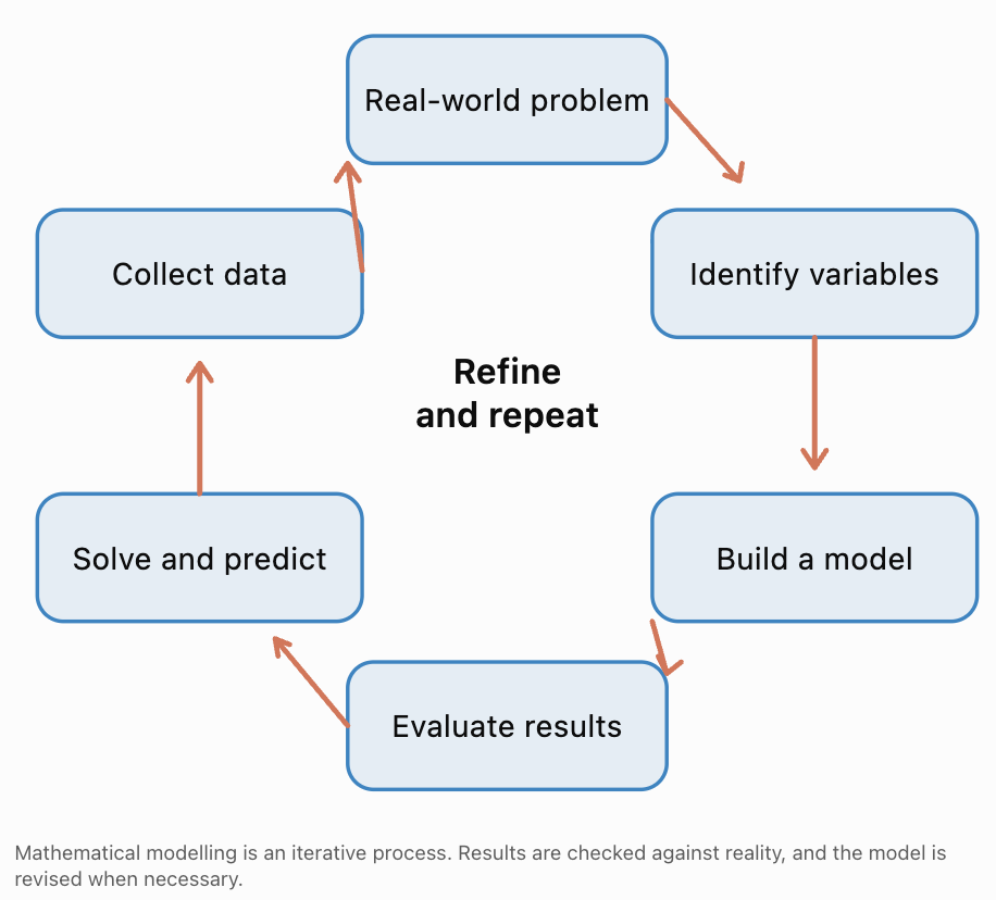
The modelling process generally involves six stages.
-
Understand the problem: Identify what needs to be calculated, explained, or predicted.
-
Define variables and assumptions: Decide which quantities matter and which simplifying assumptions are reasonable.
-
Collect and organize data: Use measurements, observations, tables, or other reliable information.
-
Choose and construct a model: Select an appropriate function and determine its parameters.
-
Use the model: Calculate values, solve equations, or make predictions.
-
Evaluate and refine: Compare predictions with observations and determine whether the model is suitable.
A model is useful when it captures the important features of a situation, even if it does not represent every detail perfectly.
Choosing Between Polynomial and Rational Models
Different mathematical relationships require different types of functions.
Polynomial Models
A polynomial function has the general form:
f(x) = aₙxⁿ + aₙ₋₁xⁿ⁻¹ + ... + a₁x + a₀
where the exponents are nonnegative integers.
Common examples include:
Linear: f(x) = mx + b
Quadratic: f(x) = ax² + bx + c
Cubic: f(x) = ax³ + bx² + cx + d
Polynomial models are often appropriate when:
-
A quantity changes at a constant rate.
-
A quantity changes at a constant second-difference rate for equally spaced inputs.
-
An area or volume depends on dimensions.
-
Motion is described using constant acceleration.
-
A smooth trend can be approximated over a limited interval.
Rational Models
A rational function has the form:
where P(x) and Q(x) are polynomials and Q(x) is not identically zero.
Rational models are often appropriate when:
-
One quantity is divided by another.
-
A relationship involves inverse variation.
-
A quantity approaches a limiting value.
-
Average cost depends on production quantity.
-
Travel time depends on speed.
-
Work rates or concentrations are involved.
Comparing Model Types
|
Situation |
Suitable model |
Reason |
|---|---|---|
|
Taxi fare with fixed fee |
Linear polynomial |
Constant cost per kilometre |
|
Projectile height |
Quadratic polynomial |
Constant acceleration |
|
Area of a square |
Quadratic polynomial |
Area depends on squared length |
|
Volume of a cube |
Cubic polynomial |
Volume depends on cubed length |
|
Travel time at varying speed |
Rational |
Time = distance/speed |
|
Average production cost |
Rational |
Total cost divided by quantity |
|
Inverse-square relationship |
Rational |
Output proportional to 1/x² |
|
Short-term curved trend |
Possibly polynomial |
Polynomial regression may approximate the data |
Important: A mathematical model should be chosen based on the relationship and the evidence, not merely because its graph resembles the data.
Identifying Patterns in Data
Before choosing a model, we should examine how the output changes as the input changes.
Constant First Differences
Consider:
|
x |
y |
|---|---|
|
0 |
3 |
|
1 |
7 |
|
2 |
11 |
|
3 |
15 |
|
4 |
19 |
The first differences are:
7 − 3 = 4
11 − 7 = 4
15 − 11 = 4
19 − 15 = 4
The first differences are constant.
This suggests a linear model:
y = 4x + 3
Constant Second Differences
Consider:
|
x |
y |
First difference |
Second difference |
|---|---|---|---|
|
0 |
2 |
— |
— |
|
1 |
5 |
3 |
— |
|
2 |
10 |
5 |
2 |
|
3 |
17 |
7 |
2 |
|
4 |
26 |
9 |
2 |
The first differences are 3, 5, 7, 9.
The second differences are constant at 2.
This suggests a quadratic model.
In fact:
y = x² + 2x + 2
Recognizing Inverse Relationships
Consider:
|
x |
y |
|---|---|
|
1 |
24 |
|
2 |
12 |
|
3 |
8 |
|
4 |
6 |
|
6 |
4 |
The product xy is constant:
1 × 24 = 24
2 × 12 = 24
3 × 8 = 24
This suggests:
y = 24/x
which is a rational model.
Recognizing a Limiting Value
Consider:
|
x |
y |
|---|---|
|
1 |
30 |
|
2 |
20 |
|
4 |
15 |
|
5 |
14 |
|
10 |
12 |
The values decrease toward 10.
This suggests a model of the form:
y = a/x + 10
Using x = 1, y = 30:
30 = a + 10
a = 20
Therefore:
y = 20/x + 10
The horizontal asymptote y = 10 represents the limiting value.
A Caution About Patterns
Constant differences identify polynomial degree only under suitable conditions, including equally spaced x-values and exact data generated by a polynomial.
Real measurements contain uncertainty and noise, so differences are rarely perfectly constant. In practice, graphs, regression, residuals, and scientific understanding should be considered together.
Creating Mathematical Models from Data
Once we identify a pattern, the next step is to construct an equation.
This may involve solving for unknown coefficients, using a regression tool, or applying a known scientific relationship.
Worked Example 1: Building a Linear Model
A delivery company records the following costs:
|
Distance (km) |
Cost ($) |
|---|---|
|
2 |
11 |
|
4 |
17 |
|
6 |
23 |
|
8 |
29 |
Find a model for delivery cost.
Step 1: Identify the relationship.
The cost increases by $6 whenever distance increases by 2 km.
Therefore, the rate of change is:
m = 6/2 = 3 dollars per kilometre.
Step 2: Use linear form.
C(d) = md + b
Substitute m = 3:
C(d) = 3d + b
Step 3: Find the fixed cost.
Using (2, 11):
11 = 3(2) + b
b = 5
Final model:
C(d) = 3d + 5
Step 4: Interpret the parameters.
-
3 represents the cost per kilometre.
-
5 represents the fixed delivery fee.
Step 5: Make a prediction.
For 12 km:
C(12) = 3(12) + 5 = 41
Predicted delivery cost: $41.
This prediction assumes the same pricing rule applies at 12 km.
Worked Example 2: Building a Quadratic Model
A student measures the height of a ball at different times.
|
Time (s) |
Height (m) |
|---|---|
|
0 |
2 |
|
1 |
17 |
|
2 |
22 |
|
3 |
17 |
|
4 |
2 |
We expect a quadratic model because the ball rises and then falls under approximately constant gravitational acceleration.
Use:
h(t) = at² + bt + c
Step 1: Find c.
At t = 0, h = 2.
Therefore:
c = 2
So:
h(t) = at² + bt + 2
Step 2: Use the point (1, 17).
17 = a + b + 2
a + b = 15
Step 3: Use the point (2, 22).
22 = 4a + 2b + 2
4a + 2b = 20
Divide by 2:
2a + b = 10
Step 4: Solve simultaneously.
2a + b = 10
a + b = 15
Subtract:
a = −5
Then:
−5 + b = 15
b = 20
Final model:
h(t) = −5t² + 20t + 2
Step 5: Verify the model.
At t = 3:
h(3) = −5(9) + 20(3) + 2
= −45 + 60 + 2
= 17
This matches the recorded height.
At t = 4:
h(4) = −80 + 80 + 2 = 2
Again, the model matches the data.
Visualizing the Model
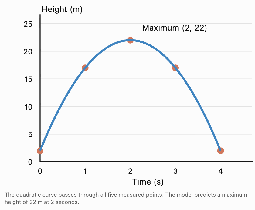
Interpretation of parameters:
-
a = −5 determines the downward curvature. In the ideal constant-acceleration model, a = −g/2.
-
b = 20 represents the initial vertical velocity in m/s.
-
c = 2 represents the initial height in metres.
The model is physically meaningful from launch until the ball reaches the ground, approximately 4.10 seconds after launch.
Worked Example 3: Building a Rational Model
A manufacturer has a fixed production cost and a constant cost per item.
The following average costs are recorded:
|
Number of items |
Average cost ($) |
|---|---|
|
20 |
50 |
|
40 |
35 |
|
60 |
30 |
|
100 |
26 |
We expect the average cost to have the form:
A(x) = a/x + b
where:
-
a represents fixed production cost.
-
b represents variable cost per item.
Step 1: Use two data points.
For x = 20:
50 = a/20 + b
For x = 40:
35 = a/40 + b
Step 2: Subtract the equations.
50 − 35 = a/20 − a/40
15 = a/40
a = 600
Step 3: Find b.
50 = 600/20 + b
50 = 30 + b
b = 20
Final model:
Step 4: Verify the other data points.
A(60) = 600/60 + 20 = 30
A(100) = 600/100 + 20 = 26
Both match.
Interpretation:
The fixed cost is $600.
The variable cost is $20 per item.
As production increases, average cost approaches $20.
The horizontal asymptote is:
y = 20
For this application, x is a positive whole number.
Worked Example 4: Building a Cubic Model from Geometry
A company manufactures open-top boxes by cutting squares of side length x from each corner of a rectangular sheet measuring 30 cm by 20 cm.
After folding the sides upward:
-
Height = x
-
Length = 30 − 2x
-
Width = 20 − 2x
The volume is:
V(x) = x(30 − 2x)(20 − 2x)
Expand:
(30 − 2x)(20 − 2x) = 600 − 100x + 4x²
Therefore:
This is a cubic polynomial model.
Determine the practical domain.
All dimensions must be positive:
x > 0
30 − 2x > 0 gives x < 15.
20 − 2x > 0 gives x < 10.
Therefore:
0 < x < 10
Although the polynomial is mathematically defined for all real x, only this interval represents a physical box.
Calculate the volume when x = 4.
V(4) = 4(30 − 8)(20 − 8)
= 4(22)(12)
= 1056 cm³
This example shows how geometry naturally produces polynomial models and how practical restrictions differ from a function's mathematical domain.
Interpreting Model Parameters
Parameters are constants within an equation that control the model's behaviour.
Understanding them allows us to explain the relationship rather than simply perform calculations.
|
Model |
Parameters |
Interpretation |
|---|---|---|
|
y = mx + b |
m, b |
Rate of change and initial value |
|
y = ax² + bx + c |
a, b, c |
Curvature, linear contribution, initial value |
|
y = a(x − h)² + k |
a, h, k |
Opening/scale and vertex location |
|
y = a/x + b |
a, b |
Inverse contribution and limiting value |
|
y = a/(x − h) + k |
a, h, k |
Scale/orientation and asymptote positions |
Worked Example 5: Interpreting Changes in Parameters
Consider two average-cost models:
Company A:
A(x) = 400/x + 15
Company B:
B(x) = 700/x + 12
Company A has lower fixed costs but higher variable costs.
Company B has higher fixed costs but lower variable costs.
Find the production quantity where their average costs are equal.
400/x + 15 = 700/x + 12
15 − 12 = 700/x − 400/x
3 = 300/x
3x = 300
x = 100
At 100 items, both companies have the same average cost:
A(100) = 4 + 15 = $19
B(100) = 7 + 12 = $19
For fewer than 100 items, Company A has the lower average cost.
For more than 100 items, Company B has the lower average cost.
This illustrates how parameters can influence real business decisions.
Evaluating the Accuracy of Mathematical Models
A model is not necessarily reliable simply because it produces an equation.
We must compare its predictions with observed data.
One of the most important ideas is the residual.
A residual is the difference between an observed value and the value predicted by a model.
Residual = Observed value − Predicted value
Or:
e = y − ŷ
where:
-
y is the observed value.
-
ŷ is the predicted value.
-
e is the residual.
A positive residual means the model predicted too low.
A negative residual means the model predicted too high.
Worked Example 6: Calculating Residuals
Suppose a model predicts the number of visitors to a website using:
V(t) = 100t + 500
where t is the number of weeks after a campaign begins.
The actual data are:
|
Week |
Observed visitors |
Predicted visitors |
Residual |
|---|---|---|---|
|
0 |
520 |
500 |
+20 |
|
1 |
590 |
600 |
−10 |
|
2 |
730 |
700 |
+30 |
|
3 |
780 |
800 |
−20 |
|
4 |
910 |
900 |
+10 |
For week 2:
Residual = 730 − 700 = +30
The model underestimated visitors by 30.
For week 3:
Residual = 780 − 800 = −20
The model overestimated visitors by 20.
Visualizing Residuals
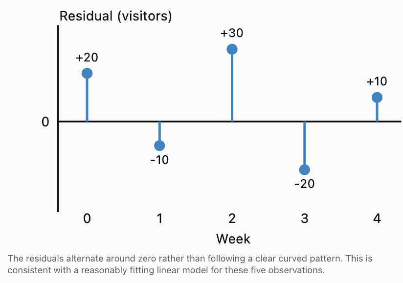
Interpreting Residual Patterns
A useful model should generally produce residuals that are small relative to the scale of the data.
We also examine whether residuals follow a pattern.
-
Residuals scattered around zero suggest the model captures the main trend.
-
A curved residual pattern suggests the chosen function may be missing curvature.
-
Residuals that increase in magnitude suggest changing prediction accuracy.
-
A single unusually large residual may indicate an outlier or measurement problem.
Residuals alone cannot prove that a model is correct, but they are valuable for identifying weaknesses.
Measuring Model Accuracy
Several numerical measures can be used to compare models.
Mean Absolute Error (MAE)
The mean absolute error measures the average size of the prediction errors.
where n is the number of observations.
For the visitor data:
Absolute residuals:
20, 10, 30, 20, 10
MAE = (20 + 10 + 30 + 20 + 10)/5
MAE = 90/5
MAE = 18 visitors.
This means the model's predictions differ from the observations by an average of 18 visitors.
Mean Squared Error (MSE)
Mean squared error gives more weight to large errors.
For the same data:
MSE = (400 + 100 + 900 + 400 + 100)/5
MSE = 1900/5
MSE = 380 visitors².
Root Mean Squared Error (RMSE)
RMSE is the square root of MSE:
RMSE = √380
RMSE ≈ 19.49 visitors.
RMSE has the same units as the original output variable, making it easier to interpret than MSE.
Coefficient of Determination (R²)
R² measures how much of the variation in the observed outputs is accounted for by a model relative to predicting their mean.
For a model evaluated on a dataset:
where ȳ is the mean observed output.
Values close to 1 often indicate a strong fit on the evaluated dataset.
However, R² does not establish that a model is scientifically correct, nor does it guarantee accurate future predictions. R² can also be negative when predictions are worse than using the observed mean.
Worked Example 7: Comparing Two Models
Suppose the following data describe a company's revenue over five years.
|
Year t |
Revenue ($ thousands) |
|---|---|
|
0 |
10 |
|
1 |
15 |
|
2 |
22 |
|
3 |
31 |
|
4 |
42 |
We consider two models.
Model A: Linear
L(t) = 8t + 8
Model B: Quadratic
Q(t) = t² + 4t + 10
Calculate predictions.
|
t |
Observed |
Linear prediction |
Quadratic prediction |
|---|---|---|---|
|
0 |
10 |
8 |
10 |
|
1 |
15 |
16 |
15 |
|
2 |
22 |
24 |
22 |
|
3 |
31 |
32 |
31 |
|
4 |
42 |
40 |
42 |
Evaluate Model A.
Residuals:
2, −1, −2, −1, 2
MAE:
(2 + 1 + 2 + 1 + 2)/5 = 1.6
Evaluate Model B.
All residuals are zero.
MAE = 0
Therefore, Model B fits the observed data exactly.
Does this guarantee Model B is the better long-term model?
No.
The quadratic model perfectly fits these five observations, but future revenue may be affected by competition, economic conditions, market saturation, or other factors.
An exact fit to past data does not guarantee accurate extrapolation.
When evaluating models, consider mathematical accuracy, simplicity, assumptions, and whether the relationship makes sense in context.
Interpolation and Extrapolation
Mathematical models are often used to estimate values that were not directly measured.
There are two important types of prediction.
Interpolation means predicting within the range of observed input values.
Extrapolation means predicting outside the observed range.
Suppose measurements were collected for x-values between 0 and 10.
Predicting at x = 6.5 is interpolation.
Predicting at x = 25 is extrapolation.
Extrapolation is generally more uncertain because the relationship may change beyond the observed range.
For example, a quadratic model of company revenue might fit five years of data but predict unrealistic revenue after 50 years.
A good modelling report should clearly distinguish between predictions supported by observed data and predictions that extend beyond it.
Solving Real-World Problems Using Models
After creating and evaluating a model, we can use it to answer practical questions.
These often involve solving equations, identifying maximum or minimum values, or comparing different functions.
Worked Example 8: Break-Even Analysis
A company sells each product for $40.
Its total cost is:
C(x) = 500 + 15x
Revenue is:
R(x) = 40x
Profit is revenue minus cost:
P(x) = R(x) − C(x)
P(x) = 40x − (500 + 15x)
P(x) = 25x − 500
Find the break-even quantity.
At break-even:
P(x) = 0
25x − 500 = 0
25x = 500
x = 20
The company breaks even when it sells 20 items.
Find the profit from 80 items.
P(80) = 25(80) − 500
= 2000 − 500
= $1,500
Interpretation: Selling more than 20 items produces a positive profit under this model.
Worked Example 9: Solving a Rational Cost Model
A manufacturer's average cost per item is:
A(x) = 900/x + 18
The company wants average cost to be no more than $30.
Solve:
900/x + 18 ≤ 30
For the practical domain x > 0:
900/x ≤ 12
Multiply both sides by positive x:
900 ≤ 12x
x ≥ 75
Therefore, the company must produce at least 75 items to achieve an average cost of $30 or less.
The positivity of x matters when multiplying an inequality by x.
Worked Example 10: Optimizing a Polynomial Model
A farmer has 80 metres of fencing to create a rectangular enclosure along a straight wall. The wall forms one side, so fencing is required for only three sides.
Let x be the width perpendicular to the wall.
The two widths use 2x metres of fencing.
The remaining fenced length is:
80 − 2x
Area:
A(x) = x(80 − 2x)
Expand:
A(x) = −2x² + 80x
This is a downward-opening quadratic.
Find the maximum area.
Vertex x-coordinate:
x = −80/[2(−2)]
x = 20
Length:
80 − 2(20) = 40
Maximum area:
A(20) = 20 × 40
= 800 m²
Conclusion: The farmer should construct an enclosure 20 metres wide and 40 metres long to maximize area.
The practical domain is 0 < x < 40.
Evaluating the Limitations of Models
Every mathematical model relies on assumptions.
For example:
A projectile model may ignore air resistance.
A production-cost model may assume fixed costs and constant material prices.
A population model may assume stable environmental conditions.
A travel-time model may assume constant speed.
These assumptions simplify calculations, but they may reduce accuracy.
Questions to Ask When Evaluating a Model
-
Does the model match the observed data reasonably well?
-
Are its parameters meaningful?
-
Does it predict realistic values?
-
Are the domain and range appropriate for the situation?
-
Are there outliers or systematic residual patterns?
-
Is the model unnecessarily complicated?
-
Are predictions being made outside the observed data?
-
Could important external factors change the relationship?
A useful model is not necessarily the most complicated model. Often, a simpler model is preferable when it explains the data adequately and is easier to interpret.
Common Mistakes
Mistake 1: Choosing a Model Based Only on Its Graph
A graph may resemble a quadratic curve, but this does not prove the relationship is quadratic.
Examine the variables, data patterns, and underlying mathematical relationship.
Mistake 2: Assuming All Curved Relationships Are Quadratic
A curved relationship could be cubic, rational, exponential, logarithmic, or another function type.
For example, travel time for a fixed distance follows t = d/v, not a quadratic model.
Mistake 3: Ignoring Units
A parameter has meaning only when interpreted with appropriate units.
In C(x) = 5x + 100, the coefficient 5 might represent dollars per item, while 100 represents dollars.
Mistake 4: Using an Incorrect Domain
A production quantity cannot be negative.
A time after launch cannot be negative.
A physical length must be positive.
The mathematical domain and practical domain may be different.
Mistake 5: Confusing a Perfect Fit with a Reliable Model
A polynomial can fit a small number of data points exactly while giving unrealistic predictions outside the observed range.
Mistake 6: Confusing Residual Signs
Residual = Observed − Predicted.
A positive residual means the model underestimated the observed value.
A negative residual means the model overestimated it.
Mistake 7: Ignoring Asymptotes in Rational Models
An asymptote may represent an important limiting value.
For A(x) = 500/x + 12, the horizontal asymptote y = 12 represents the variable cost per item.
Mistake 8: Treating Predictions as Certainties
Models are simplified representations of reality. Their predictions depend on assumptions, data quality, and the stability of the relationship.
Mistake 9: Forgetting to Interpret the Answer
Solving x = 75 is not enough.
A complete conclusion should explain that 75 items must be produced to meet the target average cost.
Key Terms
-
Mathematical Model: A mathematical representation of a real-world situation.
-
Polynomial Model: A model using a polynomial function.
-
Rational Model: A model using a quotient of polynomial functions.
-
Independent Variable: The input quantity.
-
Dependent Variable: The output quantity.
-
Parameter: A constant in a model that controls its behaviour.
-
Linear Model: A model with a constant rate of change.
-
Quadratic Model: A second-degree polynomial model.
-
Cubic Model: A third-degree polynomial model.
-
Inverse Variation: A relationship where one quantity is proportional to the reciprocal of another.
-
Regression: A method of estimating a model's parameters from data.
-
Residual: The difference between an observed value and a predicted value.
-
Mean Absolute Error (MAE): The average absolute prediction error.
-
Mean Squared Error (MSE): The average squared prediction error.
-
Root Mean Squared Error (RMSE): The square root of MSE.
-
Coefficient of Determination (R²): A measure comparing prediction error with variation around the observed mean.
-
Interpolation: Estimating a value within the observed input range.
-
Extrapolation: Estimating a value outside the observed input range.
-
Asymptote: A line approached by a graph in a limiting situation.
-
Practical Domain: The input values that make sense in the real-world context.
-
Break-Even Point: The quantity at which revenue equals cost.
-
Optimization: Finding the greatest or least possible value under given conditions.
-
Assumption: A simplifying condition accepted when constructing a model.
-
Model Validation: Evaluating how well a model performs against relevant observations, preferably including data not used to fit it.
Key Takeaways
-
Mathematical modelling connects real-world situations with mathematical functions.
-
Polynomial models are useful for relationships involving constant rates, area, volume, motion, and curved trends.
-
Rational models are useful for ratios, rates, average costs, and inverse relationships.
-
Data tables and graphs help identify possible models.
-
Constant first differences suggest a linear relationship for equally spaced inputs.
-
Constant second differences suggest a quadratic relationship under suitable conditions.
-
Model parameters should be interpreted using real-world units.
-
Residuals measure differences between observed and predicted values.
-
MAE, MSE, RMSE, and R² can help evaluate model accuracy.
-
A model that fits past data perfectly may still make poor future predictions.
-
Interpolation is generally more reliable than extrapolation.
-
Practical domains may be more restricted than mathematical domains.
-
Models can be used to find break-even points, optimize quantities, and make predictions.
-
Good mathematical modelling requires interpretation, evaluation, and awareness of limitations.
Check Your Understanding
Question 1: Choosing a Model
Choose a suitable polynomial or rational model for each situation and explain why.
a) The height of a ball thrown vertically upward.
b) The time needed to travel 300 km at different constant speeds.
c) The area of a square as its side length changes.
d) The average cost per item when there is a fixed production cost.
Question 2: Identifying a Linear Model
The following data show the cost of a service.
|
Hours |
Cost ($) |
|---|---|
|
1 |
45 |
|
2 |
70 |
|
3 |
95 |
|
4 |
120 |
Find a linear model and interpret its parameters.
Question 3: Creating a Quadratic Model
A quadratic function passes through:
(0, 3), (1, 8), and (2, 11).
Find an equation of the form:
f(x) = ax² + bx + c
Question 4: Creating a Rational Model
The average cost of producing x items follows:
A(x) = a/x + b
Given:
A(20) = 40
A(40) = 30
Find a and b, then calculate A(100).
Question 5: Evaluating Residuals
A model predicts the following values:
|
Observed |
Predicted |
|---|---|
|
12 |
10 |
|
18 |
20 |
|
25 |
24 |
|
31 |
34 |
a) Calculate the residuals.
b) Calculate the MAE.
c) Explain what the MAE means.
Question 6: Interpolation and Extrapolation
A scientist collects data for temperatures between 10°C and 40°C.
Classify the following predictions as interpolation or extrapolation.
a) Predicting at 25°C.
b) Predicting at 60°C.
c) Predicting at 5°C.
Which predictions require greater caution?
Question 7: Interpreting Parameters
A company uses:
C(x) = 750 + 18x
where x is the number of items produced.
a) What does 750 represent?
b) What does 18 represent?
c) Calculate the cost of producing 150 items.
d) Write an average-cost function.
Question 8: Solving a Rational Model
A factory's average cost is:
A(x) = 1200/x + 25
How many items must be produced for average cost to be no more than $40?
Question 9: Optimization
A rectangular garden has a perimeter of 60 m.
a) Write an area function in terms of one side length x.
b) Find the maximum area.
c) Determine the garden dimensions that produce this area.
Question 10: Challenge — Comparing Two Models
Two companies have average-cost functions:
A(x) = 300/x + 18
B(x) = 600/x + 15
a) Find the production quantity where average costs are equal.
b) Calculate the average cost at that quantity.
c) Determine which company is cheaper for 50 items.
d) Determine which company is cheaper for 200 items.
e) Explain why the preferred company changes as production increases.
Fully Worked Answers
Answer 1: Choosing Models
a) Quadratic polynomial.
Under constant gravitational acceleration, height changes quadratically with time.
b) Rational.
Time = Distance / Speed, so t(v) = 300/v.
c) Quadratic polynomial.
A(s) = s².
d) Rational.
Average cost is total cost divided by production quantity.
Answer 2: Linear Model
The cost increases by $25 for each additional hour.
Therefore:
m = 25
Use:
C = 25h + b
Substitute (1, 45):
45 = 25 + b
b = 20
Final model:
C = 25h + 20
The hourly charge is $25.
The fixed fee is $20.
Answer 3: Quadratic Model
Use:
f(x) = ax² + bx + c
At (0, 3):
c = 3
At (1, 8):
a + b + 3 = 8
a + b = 5
At (2, 11):
4a + 2b + 3 = 11
4a + 2b = 8
2a + b = 4
Subtract:
(2a + b) − (a + b) = 4 − 5
a = −1
Then:
−1 + b = 5
b = 6
Final model:
f(x) = −x² + 6x + 3
Answer 4: Rational Model
Given:
A(x) = a/x + b
Using A(20) = 40:
40 = a/20 + b
Using A(40) = 30:
30 = a/40 + b
Subtract:
10 = a/40
a = 400
Substitute:
40 = 400/20 + b
40 = 20 + b
b = 20
Final model:
A(x) = 400/x + 20
At x = 100:
A(100) = 400/100 + 20
= 4 + 20
= $24 per item.
Answer 5: Residuals
Residual = Observed − Predicted.
Residuals:
12 − 10 = +2
18 − 20 = −2
25 − 24 = +1
31 − 34 = −3
Absolute residuals:
2, 2, 1, 3
MAE = (2 + 2 + 1 + 3)/4
MAE = 8/4
MAE = 2.
The model's predictions differ from the observations by an average of 2 units.
Answer 6: Interpolation and Extrapolation
Observed range: 10°C to 40°C.
a) 25°C is interpolation.
b) 60°C is extrapolation.
c) 5°C is extrapolation.
Predictions at 60°C and 5°C require greater caution because they are outside the observed range.
Answer 7: Interpreting Parameters
Given:
C(x) = 750 + 18x
a) 750 represents the fixed cost of $750.
b) 18 represents the variable cost of $18 per item.
c) At 150 items:
C(150) = 750 + 18(150)
= 750 + 2700
= $3,450
d) Average cost:
A(x) = C(x)/x
A(x) = (750 + 18x)/x
Final model:
A(x) = 750/x + 18
for x > 0.
Answer 8: Rational Model
Given:
A(x) = 1200/x + 25
We require:
1200/x + 25 ≤ 40
Subtract 25:
1200/x ≤ 15
Since x > 0:
1200 ≤ 15x
x ≥ 80
Answer: At least 80 items must be produced.
Answer 9: Optimization
Perimeter:
2L + 2W = 60
Divide by 2:
L + W = 30
Let W = x.
Then:
L = 30 − x
Area:
A(x) = x(30 − x)
Expand:
A(x) = −x² + 30x
The parabola opens downward.
Vertex:
x = −30/[2(−1)]
x = 15
Length:
30 − 15 = 15
Maximum area:
15 × 15 = 225 m²
Answer: A 15 m by 15 m square gives the maximum area of 225 m².
Answer 10: Comparing Companies
Given:
A(x) = 300/x + 18
B(x) = 600/x + 15
a) Equal average costs
300/x + 18 = 600/x + 15
18 − 15 = 600/x − 300/x
3 = 300/x
3x = 300
x = 100
b) Average cost at 100 items
A(100) = 300/100 + 18
= $21
B(100) = 600/100 + 15
= $21
c) At 50 items
A(50) = 300/50 + 18 = $24
B(50) = 600/50 + 15 = $27
Company A is cheaper.
d) At 200 items
A(200) = 300/200 + 18 = $19.50
B(200) = 600/200 + 15 = $18
Company B is cheaper.
e) Interpretation
Company A has lower fixed costs but higher variable costs.
Company B has higher fixed costs but lower variable costs.
At low production quantities, Company A's lower fixed costs make it cheaper.
At high production quantities, Company B's lower variable cost becomes more important.
The crossover occurs at 100 items.
This completes Real-World Modelling, covering all five learning targets: selecting polynomial and rational models, constructing models from data, evaluating accuracy, interpreting parameters, and solving practical problems using mathematical functions.
5. Comprehensive Problem Solving
Learning outcomes
- I can solve multi-step problems involving polynomial and rational functions.
- I can select appropriate algebraic techniques.
- I can justify my mathematical reasoning.
- I can communicate solutions clearly.
- I can connect concepts from throughout the course.
Introduction
Throughout the study of polynomial and rational functions, we have developed a wide range of mathematical skills. We have learned how to simplify expressions, solve equations, factor polynomials, analyze graphs, identify asymptotes, apply transformations, and construct mathematical models.
Each of these skills is valuable on its own. However, many challenging mathematical problems cannot be solved using only one technique.
A problem involving a rational function might require us to factor a polynomial, determine domain restrictions, solve an equation, reject an extraneous solution, and interpret the final answer.
Similarly, a real-world optimization problem might require us to create a quadratic model, determine its domain, calculate a maximum value, and explain why the result makes sense.
Comprehensive problem solving involves recognizing which mathematical tools are needed, combining them efficiently, and communicating the reasoning behind every important step.
The goal is not simply to obtain a correct numerical answer. A complete mathematical solution should explain why the chosen method works, demonstrate accurate calculations, verify the result, and interpret its meaning.
This lesson brings together the major concepts from polynomial and rational functions through progressively more challenging, multi-step problems.
A Systematic Approach to Mathematical Problem Solving
Complex problems become more manageable when we follow a clear process.
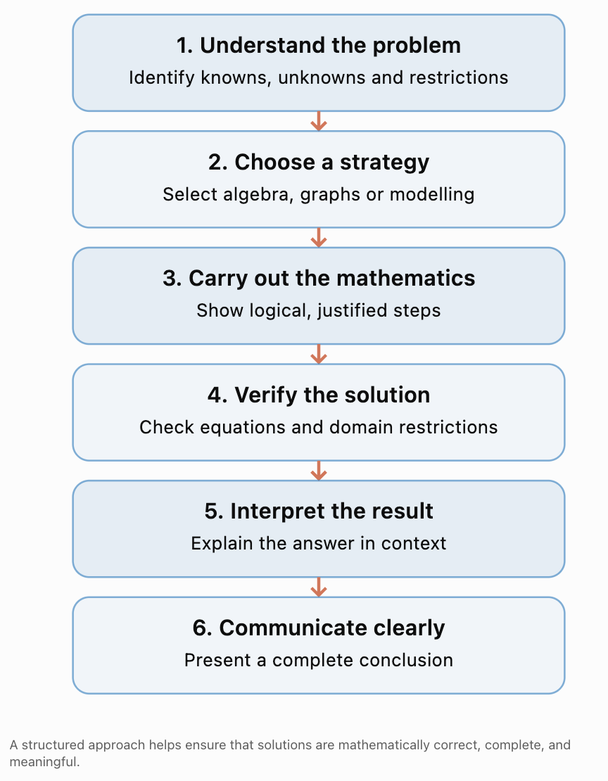
Step 1: Understand the Problem
Before calculating, identify:
-
What information is given?
-
What quantity must be found?
-
Which variables are involved?
-
Are there domain restrictions?
-
Is an exact or approximate answer required?
-
Does the answer need to be interpreted in a real-world context?
Step 2: Select an Appropriate Technique
Different problems suggest different methods.
|
Problem characteristic |
Useful technique |
|---|---|
|
Polynomial equation |
Factoring, quadratic formula, substitution |
|
Higher-degree polynomial |
Grouping, factor theorem, synthetic division |
|
Rational equation |
LCD multiplication and solution checking |
|
Polynomial inequality |
Factoring and sign analysis |
|
Rational inequality |
Critical values and sign charts |
|
Graph features |
Intercepts, extrema, asymptotes, end behaviour |
|
Transformed function |
Parent functions and transformation rules |
|
Maximum or minimum |
Vertex method, graphing, or calculus |
|
Real-world data |
Function modelling and validation |
|
Comparing two models |
Solve their intersection equation |
Step 3: Justify Each Step
A mathematical solution should explain important decisions.
For example:
“We factor the numerator and denominator to identify excluded values and simplify the rational expression.”
This is more informative than simply writing several lines of unexplained algebra.
Step 4: Verify the Answer
Check that solutions:
-
Satisfy the original equation.
-
Do not make denominators zero.
-
Meet any physical restrictions.
-
Have appropriate units.
-
Are consistent with the graph or model.
Step 5: Communicate the Conclusion
A final answer should state what was found.
Instead of writing only:
x = 80
write:
“The company must produce at least 80 items to achieve the required average cost.”
This makes the mathematical result meaningful.
Connecting the Main Ideas of the Course
Polynomial and rational functions are closely related.
A rational function is formed by dividing one polynomial by another:
f(x) = P(x)/Q(x)
Many rational problems therefore require polynomial techniques.
For example, solving:
requires us to factor the numerator:
(x − 3)(x + 3) = 0
The solutions are x = 3 and x = −3.
However, the domain also requires x ≠ 1.
The same problem involves factoring, solving equations, and checking domain restrictions.
The following sections demonstrate how these skills combine.
Worked Example 1: A Multi-Step Polynomial Equation
Solve:
x⁴ − 5x² + 4 = 0
Step 1: Identify the Structure
This is a fourth-degree polynomial equation, but it contains only even powers of x.
We can use substitution.
Let:
u = x²
Then:
x⁴ = u²
The equation becomes:
u² − 5u + 4 = 0
Step 2: Factor
(u − 1)(u − 4) = 0
Therefore:
u = 1 or u = 4
Step 3: Substitute Back
Since u = x²:
x² = 1 or x² = 4
Taking square roots:
x = ±1 or x = ±2
Step 4: Verify
For x = 2:
2⁴ − 5(2²) + 4
= 16 − 20 + 4
= 0
The other solutions also satisfy the original equation because only even powers appear.
Final answer:
x = −2, −1, 1, 2
Why this method works: Substitution transforms a fourth-degree equation into a quadratic equation that is easier to factor.
Worked Example 2: Factoring a Cubic Polynomial
Solve:
x³ − 4x² − x + 4 = 0
Step 1: Group Terms
(x³ − 4x²) + (−x + 4) = 0
Factor each group:
x²(x − 4) − (x − 4) = 0
Step 2: Factor the Common Binomial
(x − 4)(x² − 1) = 0
Use the difference of squares:
(x − 4)(x − 1)(x + 1) = 0
Step 3: Solve
x − 4 = 0 gives x = 4.
x − 1 = 0 gives x = 1.
x + 1 = 0 gives x = −1.
Final answer:
x = −1, 1, 4
Verification
Substitute x = 4:
64 − 64 − 4 + 4 = 0
Therefore, x = 4 is valid.
The factored form confirms that all three solutions satisfy the equation.
Connection: This problem combines polynomial grouping, the difference-of-squares identity, and the zero-product property.
Worked Example 3: Polynomial Division and the Factor Theorem
A polynomial is given by:
P(x) = 2x³ − 3x² − 11x + 6
Determine whether x − 3 is a factor, and solve P(x) = 0.
Step 1: Apply the Factor Theorem
The factor theorem states:
x − a is a factor of P(x) if P(a) = 0.
Evaluate:
P(3) = 2(27) − 3(9) − 11(3) + 6
= 54 − 27 − 33 + 6
= 0
Therefore, x − 3 is a factor.
Step 2: Divide the Polynomial
Use synthetic division with 3.
Coefficients:
2, −3, −11, 6
|
Step |
Coefficients |
|---|---|
|
Original |
2, −3, −11, 6 |
|
Bring down |
2 |
|
Multiply and add |
2, 3 |
|
Continue |
2, 3, −2 |
|
Remainder |
0 |
The quotient is:
2x² + 3x − 2
Therefore:
P(x) = (x − 3)(2x² + 3x − 2)
Step 3: Factor the Quadratic
2x² + 3x − 2 = (2x − 1)(x + 2)
Therefore:
P(x) = (x − 3)(2x − 1)(x + 2)
Step 4: Solve
x = 3
x = 1/2
x = −2
Final answer:
x = −2, 1/2, 3
Connection: The factor theorem identifies a factor, polynomial division reduces the degree, and quadratic factoring completes the solution.
Worked Example 4: Solving a Rational Equation and Rejecting Extraneous Solutions
Solve:
Step 1: Identify Domain Restrictions
Denominators cannot equal zero.
x − 1 ≠ 0, so x ≠ 1.
x + 1 ≠ 0, so x ≠ −1.
Therefore:
Restrictions: x ≠ 1 and x ≠ −1.
Step 2: Find the Least Common Denominator
The LCD is:
(x − 1)(x + 1)
Multiply every term by the LCD:
(x + 2)(x + 1) = 3(x + 1) + x(x − 1)
Step 3: Expand
Left side:
x² + 3x + 2
Right side:
3x + 3 + x² − x
= x² + 2x + 3
Therefore:
x² + 3x + 2 = x² + 2x + 3
Subtract x² from both sides:
3x + 2 = 2x + 3
x = 1
Step 4: Check the Solution
The algebra produced x = 1.
However, the original equation contains denominators of x − 1.
At x = 1, those denominators become zero.
Therefore, x = 1 is an extraneous solution.
Final answer: No solution.
Why This Happens
Multiplying by an expression containing a variable can produce candidate solutions that do not belong to the original equation's domain.
This is why domain restrictions must be identified before solving and checked afterward.
Worked Example 5: Simplifying a Rational Function with a Hole
Consider:
Determine:
a) The domain.
b) Any holes or vertical asymptotes.
c) The intercepts.
d) The horizontal asymptote.
Step 1: Factor
Numerator:
x² − 4 = (x − 2)(x + 2)
Denominator:
x² − x − 2 = (x − 2)(x + 1)
Therefore:
Step 2: Identify Restrictions
From the original denominator:
x ≠ 2
x ≠ −1
Step 3: Simplify
Cancel the common factor x − 2:
but retain both original restrictions.
Step 4: Identify the Hole
The cancelled factor x − 2 indicates a removable discontinuity at x = 2.
Calculate the corresponding y-value using the simplified expression:
f(2) = (2 + 2)/(2 + 1) = 4/3
Hole: (2, 4/3).
Step 5: Identify the Vertical Asymptote
The remaining denominator is zero when:
x + 1 = 0
x = −1
Vertical asymptote: x = −1.
Step 6: Find Intercepts
For the x-intercept:
x + 2 = 0
x = −2
Therefore:
(−2, 0)
For the y-intercept:
f(0) = 2/1 = 2
Therefore:
(0, 2)
Step 7: Find the Horizontal Asymptote
The simplified numerator and denominator both have degree 1.
The leading coefficient ratio is 1/1.
Horizontal asymptote: y = 1.
Summary
|
Feature |
Result |
|---|---|
|
Domain |
x ≠ −1, 2 |
|
Hole |
(2, 4/3) |
|
Vertical asymptote |
x = −1 |
|
Horizontal asymptote |
y = 1 |
|
x-intercept |
(−2, 0) |
|
y-intercept |
(0, 2) |
Connection: This problem combines factoring, rational simplification, domain restrictions, discontinuities, intercepts, and asymptotic behaviour.
Worked Example 6: Solving a Rational Inequality
Solve:
Step 1: Identify Critical Values
The numerator equals zero when:
x − 3 = 0
x = 3
The denominator equals zero when:
x + 2 = 0
x = −2
These values divide the number line into three intervals.
Step 2: Test the Intervals
|
Interval |
Test value |
Numerator sign |
Denominator sign |
Fraction sign |
|---|---|---|---|---|
|
x < −2 |
−3 |
Negative |
Negative |
Positive |
|
−2 < x < 3 |
0 |
Negative |
Positive |
Negative |
|
x > 3 |
4 |
Positive |
Positive |
Positive |
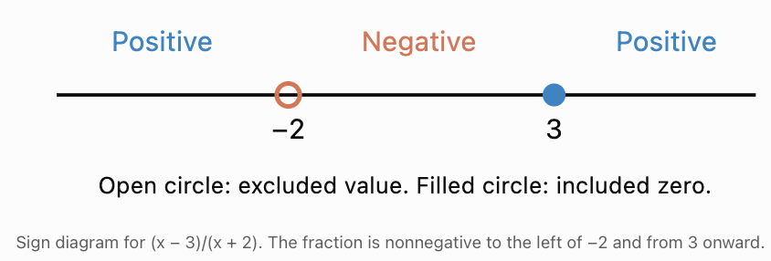
Step 3: Select the Correct Intervals
We require values greater than or equal to zero.
The fraction is positive when x < −2 or x > 3.
At x = 3, the fraction equals zero, so x = 3 is included.
At x = −2, the function is undefined, so x = −2 is excluded.
Final answer:
Why this method works: A rational expression can change sign at zeros of its numerator or denominator. Testing the intervals between these critical values determines where the inequality holds.
Worked Example 7: Complete Analysis of a Rational Function
Analyze:
Determine its domain, intercepts, asymptotes, sign intervals, and end behaviour.
Step 1: Domain
The denominator is zero when x = 1.
Therefore:
Domain: x ≠ 1.
Step 2: Intercepts
Set the numerator equal to zero:
x² − 4 = 0
(x − 2)(x + 2) = 0
x = −2 or x = 2
x-intercepts:
(−2, 0) and (2, 0).
For the y-intercept:
f(0) = (−4)/(−1) = 4
y-intercept:
(0, 4).
Step 3: Vertical Asymptote
At x = 1, the denominator is zero and the numerator is −3, not zero.
Therefore:
Vertical asymptote: x = 1.
Step 4: Oblique Asymptote
The numerator's degree is one greater than the denominator's degree.
Use polynomial division:
As x approaches positive or negative infinity, the final fraction approaches zero.
Therefore:
Oblique asymptote: y = x + 1.
Step 5: Positive and Negative Intervals
Factor the function:
Critical values:
−2, 1, 2.
Test each interval.
|
Interval |
Test x |
Sign |
|---|---|---|
|
(−∞, −2) |
−3 |
Negative |
|
(−2, 1) |
0 |
Positive |
|
(1, 2) |
1.5 |
Negative |
|
(2, ∞) |
3 |
Positive |
Therefore:
Positive: (−2, 1) ∪ (2, ∞).
Negative: (−∞, −2) ∪ (1, 2).
The function equals zero at x = −2 and x = 2.
Step 6: End Behaviour
Because:
f(x) = x + 1 − 3/(x − 1)
the graph approaches y = x + 1 as x becomes large in magnitude.
For large positive x, the graph lies slightly below this line.
For large negative x, it lies slightly above this line.
Step 7: Behaviour Near the Vertical Asymptote
As x approaches 1 from the left:
x − 1 is a small negative number.
−3/(x − 1) becomes very large and positive.
Therefore:
f(x) → +∞.
As x approaches 1 from the right:
−3/(x − 1) becomes very large and negative.
Therefore:
f(x) → −∞.
This information helps us sketch the two branches accurately.
Worked Example 8: Combining Transformations and Graph Features
A function is defined by:
Describe its transformations, domain, range, intercepts, and graph behaviour.
Step 1: Identify the Parent Function
The parent function is:
f(x) = 1/x
Step 2: Identify Transformations
-
Reflect in the x-axis.
-
Stretch vertically by a factor of 4.
-
Translate right 3 units.
-
Translate upward 2 units.
Step 3: Domain and Range
Vertical asymptote:
x = 3
Therefore, domain:
x ≠ 3
Horizontal asymptote:
y = 2
Therefore, range:
y ≠ 2
Step 4: x-Intercept
Set g(x) = 0:
−4/(x − 3) + 2 = 0
2 = 4/(x − 3)
2(x − 3) = 4
2x − 6 = 4
x = 5
x-intercept: (5, 0).
Step 5: y-Intercept
g(0) = −4/(−3) + 2
= 4/3 + 2
= 10/3
y-intercept: (0, 10/3).
Step 6: Graph Behaviour
The negative reciprocal coefficient means the branches lie in the upper-left and lower-right regions relative to the asymptote intersection (3, 2).
The function is increasing on both:
(−∞, 3) and (3, ∞).
It is not continuous across x = 3.
Connection: This problem combines function transformations, asymptotes, intercepts, domain, range, and monotonic behaviour.
Worked Example 9: Connecting Polynomial and Rational Models
Two manufacturers have different cost structures.
Company A has total cost:
Cₐ(x) = 400 + 20x
Company B has total cost:
Cᵦ(x) = 700 + 15x
where x is the number of items produced.
Determine which company has the lower average cost.
Step 1: Construct Average-Cost Functions
Average cost = Total cost / Number of items.
For Company A:
A(x) = (400 + 20x)/x
A(x) = 400/x + 20
For Company B:
B(x) = (700 + 15x)/x
B(x) = 700/x + 15
The practical domain is positive whole numbers.
Step 2: Find the Intersection
Set the average costs equal:
400/x + 20 = 700/x + 15
Subtract 15:
400/x + 5 = 700/x
Subtract 400/x:
5 = 300/x
Since x > 0:
5x = 300
x = 60
Step 3: Calculate the Equal Cost
A(60) = 400/60 + 20
≈ $26.67
B(60) = 700/60 + 15
≈ $26.67
Step 4: Compare Other Production Quantities
At 30 items:
A(30) = 400/30 + 20 ≈ $33.33
B(30) = 700/30 + 15 ≈ $38.33
Company A is cheaper.
At 100 items:
A(100) = 400/100 + 20 = $24
B(100) = 700/100 + 15 = $22
Company B is cheaper.
Conclusion
Company A is cheaper for fewer than 60 items.
Both companies have equal average costs at 60 items.
Company B is cheaper for more than 60 items.
Connection: This problem combines linear total-cost models, rational average-cost functions, equation solving, and practical interpretation.
Worked Example 10: Polynomial Optimization
A rectangular garden is built against a wall. The farmer has 100 metres of fencing for the other three sides.
Find the dimensions that maximize the garden's area.
Step 1: Define Variables
Let x be the width perpendicular to the wall.
There are two widths and one fenced length.
Therefore:
2x + L = 100
L = 100 − 2x
Step 2: Construct the Area Function
Area = Length × Width
A(x) = x(100 − 2x)
Expand:
A(x) = −2x² + 100x
Step 3: Determine the Practical Domain
Both dimensions must be positive.
x > 0
100 − 2x > 0
x < 50
Therefore:
0 < x < 50
Step 4: Find the Maximum
The quadratic opens downward.
Its maximum occurs at the vertex:
x = −b/(2a)
x = −100/[2(−2)]
x = 25
Find the length:
L = 100 − 2(25)
L = 50
Step 5: Calculate the Maximum Area
A(25) = 25 × 50
A(25) = 1250 m²
Step 6: Interpret
The garden should be 25 metres wide and 50 metres long.
The maximum area is 1250 m².
The answer is physically valid because both dimensions are positive and the fencing totals 100 metres.
Worked Example 11: Comparing Two Mathematical Models
A company measures the revenue generated by a new product.
|
Month |
Revenue ($ thousands) |
|---|---|
|
0 |
10 |
|
1 |
16 |
|
2 |
24 |
|
3 |
34 |
|
4 |
46 |
Two possible models are proposed:
Linear model:
L(t) = 9t + 8
Quadratic model:
Q(t) = t² + 5t + 10
Determine which model better represents the data.
Step 1: Calculate Predictions
|
t |
Observed |
L(t) |
Q(t) |
|---|---|---|---|
|
0 |
10 |
8 |
10 |
|
1 |
16 |
17 |
16 |
|
2 |
24 |
26 |
24 |
|
3 |
34 |
35 |
34 |
|
4 |
46 |
44 |
46 |
Step 2: Calculate Residuals
Residual = Observed − Predicted.
Linear residuals:
2, −1, −2, −1, 2
Quadratic residuals:
0, 0, 0, 0, 0
Step 3: Calculate Mean Absolute Error
Linear model:
MAE = (2 + 1 + 2 + 1 + 2)/5
MAE = 1.6
Quadratic model:
MAE = 0
Step 4: Evaluate the Models
The quadratic model fits all five observations exactly.
It is therefore the better fit to this dataset.
However, an exact fit does not prove that revenue will continue growing quadratically.
Step 5: Make a Prediction
At t = 5:
Q(5) = 5² + 5(5) + 10
= 25 + 25 + 10
= 60
The model predicts revenue of $60,000 in month 5.
This is an extrapolation because the observed data extend only to month 4.
Conclusion: The quadratic model fits the observations better, but the prediction for month 5 should be treated as an estimate rather than a certainty.
Choosing Efficient Algebraic Strategies
An important part of advanced problem solving is choosing an efficient method.
Consider the following equations.
|
Equation |
Efficient strategy |
Reason |
|---|---|---|
|
x² − 9 = 0 |
Difference of squares |
Factors immediately |
|
x² + 6x + 5 = 0 |
Factoring |
Simple integer factors |
|
x² + 4x + 1 = 0 |
Quadratic formula |
No convenient integer factors |
|
x⁴ − 5x² + 4 = 0 |
Substitution |
Quadratic in x² |
|
x³ − 3x² − 4x + 12 = 0 |
Grouping |
Common binomial factors |
|
(x + 1)/(x − 2) = 3 |
Clear denominator |
Rational equation |
|
(x − 3)/(x + 2) > 0 |
Sign chart |
Rational inequality |
|
−2(x − 3)² + 8 |
Vertex form |
Maximum is immediately visible |
|
5/(x − 1) + 2 |
Transformation analysis |
Asymptotes immediately visible |
There is rarely only one possible method. The most efficient approach usually uses the structure of the problem rather than expanding everything immediately.
How to Communicate Mathematical Reasoning Clearly
A complete solution should have four essential parts.
1. Mathematical setup
Define variables and state relevant equations.
2. Logical working
Show enough intermediate steps to make the calculation understandable.
3. Verification
Check the result against the original equation or problem conditions.
4. Conclusion
State the answer with units and context.
Example of an Incomplete Solution
x = 25
A = 1250
Example of a Complete Solution
The garden's area is modelled by:
A(x) = −2x² + 100x
Because the quadratic coefficient is negative, the vertex gives the maximum area.
The vertex occurs at x = 25 metres.
The corresponding length is 50 metres.
Therefore, the maximum area is 1250 m², achieved with dimensions of 25 m by 50 m.
The dimensions satisfy the fencing restriction because:
2(25) + 50 = 100 metres.
The second solution demonstrates the reasoning, verification, and interpretation.
Common Mistakes
Mistake 1: Starting Calculations Without Identifying Restrictions
For rational equations, determine excluded values before multiplying by denominators.
Mistake 2: Cancelling Terms Instead of Factors
Incorrect:
(x + 3)/x = 3
Correct:
(x + 3)/x = 1 + 3/x, for x ≠ 0.
Only common factors can be cancelled.
Mistake 3: Forgetting Extraneous Solutions
Solutions produced after clearing denominators must satisfy the original equation.
Mistake 4: Applying the Zero-Product Property to a Sum
From:
(x − 2)(x + 3) = 0
we can conclude x = 2 or x = −3.
We cannot apply the same rule directly to:
(x − 2) + (x + 3) = 0.
Mistake 5: Using the Wrong Inequality Boundaries
For rational inequalities, both numerator zeros and denominator zeros matter.
Denominator zeros must always be excluded.
Mistake 6: Confusing Holes with Vertical Asymptotes
A factor cancelled from a rational expression may create a hole.
An uncancelled denominator factor may create a vertical asymptote.
Mistake 7: Ignoring Practical Domains
Negative production quantities, impossible dimensions, and times outside a physical event should not be accepted as meaningful answers.
Mistake 8: Assuming a Good Fit Guarantees Accurate Predictions
A model may describe past data well but fail when conditions change.
Mistake 9: Providing Only a Numerical Answer
Complex problems require explanations, verification, and interpretation.
Mistake 10: Choosing an Unnecessarily Complicated Method
Always examine the expression's structure before expanding, dividing, or applying formulas.
Key Terms
-
Multi-Step Problem: A problem requiring several connected mathematical operations or techniques.
-
Algebraic Strategy: A planned method for solving an equation or analysing a function.
-
Polynomial Function: A function formed from nonnegative integer powers of a variable.
-
Rational Function: A quotient of two polynomial functions.
-
Factor Theorem: A theorem stating that x − a is a factor of P(x) exactly when P(a) = 0.
-
Remainder Theorem: A theorem stating that dividing P(x) by x − a gives remainder P(a).
-
Synthetic Division: An efficient method of dividing a polynomial by a linear factor of the form x − a.
-
Zero-Product Property: If a product equals zero, at least one factor equals zero.
-
Extraneous Solution: A candidate solution that does not satisfy the original equation.
-
Domain Restriction: A value excluded from a function's domain.
-
Removable Discontinuity: A missing point in a graph caused by a removable factor.
-
Vertical Asymptote: A vertical line approached as function values become unbounded.
-
Oblique Asymptote: A nonhorizontal straight line approached by a graph at infinity.
-
Critical Value for Sign Analysis: A zero or excluded input used to divide a number line into sign intervals.
-
Optimization: Finding a maximum or minimum under specified conditions.
-
Mathematical Model: A mathematical representation of a real-world relationship.
-
Residual: Observed value minus predicted value.
-
Verification: Checking whether a result satisfies the original conditions.
-
Mathematical Justification: Explaining why a mathematical method or conclusion is valid.
-
Interpretation: Explaining the meaning of a mathematical result in its context.
Key Takeaways
-
Complex polynomial and rational problems often require several connected techniques.
-
Identifying the structure of an expression helps determine an efficient strategy.
-
Factoring is useful for solving equations, simplifying expressions, and analysing signs.
-
Substitution can simplify certain higher-degree polynomial equations.
-
Rational equations require careful attention to denominator restrictions.
-
Extraneous solutions must be rejected.
-
Rational inequalities are often solved using sign charts.
-
Holes and asymptotes represent different types of discontinuity.
-
Graph transformations help predict function behaviour without extensive calculations.
-
Polynomial and rational functions can be combined to construct real-world models.
-
Optimization problems often involve quadratic functions.
-
Model accuracy should be evaluated using observed data and residuals.
-
Mathematical solutions should include reasoning, verification, and interpretation.
-
The most useful mathematical approach is not always the longest or most complicated one.
Check Your Understanding
These questions combine concepts from throughout the polynomial and rational functions course. Show your working, explain your methods, and verify solutions where appropriate.
Question 1: Polynomial Equations
Solve:
x⁴ − 10x² + 9 = 0
Explain why substitution is an efficient strategy.
Question 2: Factor Theorem and Division
Given:
P(x) = x³ − 2x² − 5x + 6
a) Show that x − 1 is a factor.
b) Factor P(x) completely.
c) Solve P(x) = 0.
Question 3: Rational Equations
Solve:
State domain restrictions and check the result.
Question 4: Rational Simplification
Consider:
a) Factor and simplify.
b) State the domain.
c) Identify any holes and vertical asymptotes.
d) Find the x-intercept.
Question 5: Rational Inequalities
Solve:
Express your answer using interval notation and justify it with sign analysis.
Question 6: Function Transformations
Starting with f(x) = 1/x, a graph is:
-
Reflected in the x-axis.
-
Stretched vertically by a factor of 2.
-
Translated left 3 units.
-
Translated upward 4 units.
a) Write its equation.
b) Find its asymptotes.
c) Determine its domain and range.
d) Find its x-intercept.
Question 7: Complete Polynomial Analysis
Analyze:
f(x) = −x² + 8x − 12
Find its intercepts, vertex, range, increasing and decreasing intervals, and positive and negative intervals.
Question 8: Real-World Cost Comparison
Two companies have total-cost models:
C₁(x) = 500 + 12x
C₂(x) = 800 + 9x
where x is the number of products.
a) Write their average-cost functions.
b) Determine the production quantity at which average costs are equal.
c) Determine which company is cheaper at 50 items and at 200 items.
d) Explain your conclusions.
Question 9: Optimization
A rectangular enclosure is built against a wall using 120 metres of fencing for the other three sides.
a) Construct an area function.
b) Determine its practical domain.
c) Find the maximum area.
d) Find the dimensions of the enclosure.
Question 10: Integrated Challenge
A function is given by:
a) Find its domain.
b) Find its x- and y-intercepts.
c) Find its vertical asymptote.
d) Use polynomial division to determine its oblique asymptote.
e) Determine where the function is positive and negative.
f) Describe its behaviour near the vertical asymptote.
g) Explain how the results help construct an accurate graph.
Fully Worked Answers
Answer 1: Polynomial Equations
Given:
x⁴ − 10x² + 9 = 0
Let:
u = x²
Then:
u² − 10u + 9 = 0
Factor:
(u − 1)(u − 9) = 0
Therefore:
u = 1 or u = 9
Substitute back:
x² = 1 or x² = 9
Therefore:
x = −3, −1, 1, 3.
Substitution is efficient because it converts a fourth-degree equation into a quadratic equation.
All four values satisfy the original equation.
Answer 2: Factor Theorem
Given:
P(x) = x³ − 2x² − 5x + 6
a) Verify x − 1 is a factor.
Evaluate P(1):
P(1) = 1 − 2 − 5 + 6 = 0
Therefore, x − 1 is a factor.
b) Factor completely.
Divide P(x) by x − 1.
The quotient is:
x² − x − 6
Factor:
x² − x − 6 = (x − 3)(x + 2)
Therefore:
P(x) = (x − 1)(x − 3)(x + 2)
c) Solve.
Set each factor equal to zero:
x = 1, 3, −2
Final answer: x = −2, 1, 3.
Answer 3: Rational Equation
Given:
Step 1: Domain restriction
x ≠ 2.
Step 2: Multiply by x − 2.
x + 3 = 5 + 2(x − 2)
Expand:
x + 3 = 5 + 2x − 4
x + 3 = 2x + 1
x = 2
Step 3: Verify
But x = 2 makes the original denominators zero.
Therefore, the candidate is extraneous.
Final answer: No solution.
Answer 4: Rational Simplification
Given:
a) Factor.
Numerator:
(x − 3)(x + 3)
Denominator:
(x − 3)(x + 1)
Therefore:
with the original restrictions retained.
b) Domain
x ≠ 3 and x ≠ −1.
c) Hole and vertical asymptote
The cancelled factor x − 3 produces a hole at x = 3.
Its y-coordinate is:
(3 + 3)/(3 + 1) = 6/4 = 3/2
Hole: (3, 3/2).
The remaining denominator gives:
Vertical asymptote: x = −1.
d) x-intercept
x + 3 = 0
x = −3
Therefore:
x-intercept: (−3, 0).
Answer 5: Rational Inequality
Given:
Critical values:
x = −1 and x = 4.
Test the intervals.
For x < −1, both numerator and denominator are negative, giving a positive fraction.
For −1 < x < 4, the numerator is positive and denominator negative, giving a negative fraction.
For x > 4, both are positive, giving a positive fraction.
The inequality requires a strictly negative result.
Therefore:
Neither endpoint is included.
At x = −1, the expression equals zero.
At x = 4, it is undefined.
Answer 6: Function Transformations
Original:
f(x) = 1/x
a) Equation
Reflect and stretch:
−2/x
Translate left 3:
−2/(x + 3)
Translate up 4:
b) Asymptotes
Vertical: x = −3.
Horizontal: y = 4.
c) Domain and range
Domain: x ≠ −3.
Range: y ≠ 4.
d) x-intercept
Set g(x) = 0:
−2/(x + 3) + 4 = 0
4 = 2/(x + 3)
4(x + 3) = 2
4x + 12 = 2
4x = −10
x = −5/2
x-intercept: (−5/2, 0).
Answer 7: Complete Polynomial Analysis
Given:
f(x) = −x² + 8x − 12
Intercepts
Set f(x) = 0:
−x² + 8x − 12 = 0
Multiply by −1:
x² − 8x + 12 = 0
(x − 2)(x − 6) = 0
x = 2 or x = 6
x-intercepts:
(2, 0), (6, 0).
y-intercept:
f(0) = −12
Therefore:
(0, −12).
Vertex
x = −8/[2(−1)] = 4
f(4) = −16 + 32 − 12 = 4
Vertex: (4, 4).
This is a maximum because the parabola opens downward.
Range
y ≤ 4.
Increasing and decreasing
Increasing: (−∞, 4).
Decreasing: (4, ∞).
Positive and negative
Positive: (2, 6).
Negative: (−∞, 2) ∪ (6, ∞).
Answer 8: Cost Comparison
Given:
C₁(x) = 500 + 12x
C₂(x) = 800 + 9x
a) Average-cost functions
A₁(x) = 500/x + 12
A₂(x) = 800/x + 9
b) Equal average costs
500/x + 12 = 800/x + 9
3 = 300/x
3x = 300
x = 100
At 100 items, both average costs are:
500/100 + 12 = $17
800/100 + 9 = $17
c) At 50 items
A₁(50) = 500/50 + 12 = $22
A₂(50) = 800/50 + 9 = $25
Company 1 is cheaper.
At 200 items:
A₁(200) = 500/200 + 12 = $14.50
A₂(200) = 800/200 + 9 = $13
Company 2 is cheaper.
d) Interpretation
Company 1 has lower fixed costs.
Company 2 has lower variable costs.
Company 1 is preferable at lower production quantities, while Company 2 becomes preferable above 100 items.
Answer 9: Optimization
Let x represent the width perpendicular to the wall.
Two widths and one length require 120 metres of fencing.
2x + L = 120
Therefore:
L = 120 − 2x
a) Area function
A(x) = x(120 − 2x)
A(x) = −2x² + 120x
b) Practical domain
x > 0
120 − 2x > 0
x < 60
Therefore:
0 < x < 60
c) Maximum area
Vertex:
x = −120/[2(−2)]
x = 30
Length:
120 − 2(30) = 60
Maximum area:
A(30) = 30 × 60 = 1800 m²
d) Dimensions
Width: 30 m.
Length: 60 m.
The fencing requirement is satisfied:
2(30) + 60 = 120 m.
Answer 10: Integrated Challenge
Given:
a) Domain
Denominator cannot equal zero.
x − 4 ≠ 0
Therefore:
x ≠ 4.
b) Intercepts
Factor numerator:
x² − x − 6 = (x − 3)(x + 2)
x-intercepts:
x = 3 and x = −2
Therefore:
(3, 0) and (−2, 0).
y-intercept:
f(0) = −6/(−4) = 3/2
Therefore:
(0, 3/2).
c) Vertical asymptote
x = 4.
The numerator at x = 4 is:
16 − 4 − 6 = 6
Since the numerator is nonzero, x = 4 is a vertical asymptote.
d) Oblique asymptote
Divide x² − x − 6 by x − 4.
The quotient is x + 3, with remainder 6.
Therefore:
As x becomes large in magnitude, 6/(x − 4) approaches zero.
Oblique asymptote:
y = x + 3.
e) Positive and negative intervals
Factor:
Critical values:
−2, 3, 4.
Test intervals.
|
Interval |
Test value |
Sign |
|---|---|---|
|
(−∞, −2) |
−3 |
Negative |
|
(−2, 3) |
0 |
Positive |
|
(3, 4) |
3.5 |
Negative |
|
(4, ∞) |
5 |
Positive |
Therefore:
Positive: (−2, 3) ∪ (4, ∞).
Negative: (−∞, −2) ∪ (3, 4).
f) Behaviour near the vertical asymptote
Use:
f(x) = x + 3 + 6/(x − 4)
As x approaches 4 from the left:
6/(x − 4) → −∞
Therefore:
f(x) → −∞.
As x approaches 4 from the right:
6/(x − 4) → +∞
Therefore:
f(x) → +∞.
g) Constructing the graph
An accurate sketch should show:
-
x-intercepts at (−2, 0) and (3, 0).
-
y-intercept at (0, 3/2).
-
Vertical asymptote x = 4.
-
Oblique asymptote y = x + 3.
-
A left branch approaching negative infinity as x approaches 4 from below.
-
A right branch approaching positive infinity as x approaches 4 from above.
-
Both branches approaching y = x + 3 for large magnitudes of x.
These features allow us to sketch the graph without constructing a large table of values.
Final Course Connections
The study of polynomial and rational functions is built around several closely related ideas.
Algebraic structure helps us simplify expressions and solve equations.
Function behaviour helps us understand intercepts, turning points, discontinuities, asymptotes, and end behaviour.
Transformations allow us to predict graphs from familiar parent functions.
Mathematical modelling connects these functions to real-world situations.
Verification and communication ensure that solutions are valid, understandable, and meaningful.
The strongest problem solvers do not simply memorize methods. They recognize mathematical structures, choose suitable strategies, connect ideas, and explain why their conclusions are justified.
This completes Comprehensive Problem Solving, bringing together the major concepts and skills developed throughout the polynomial and rational functions course.