Applications and Function Analysis

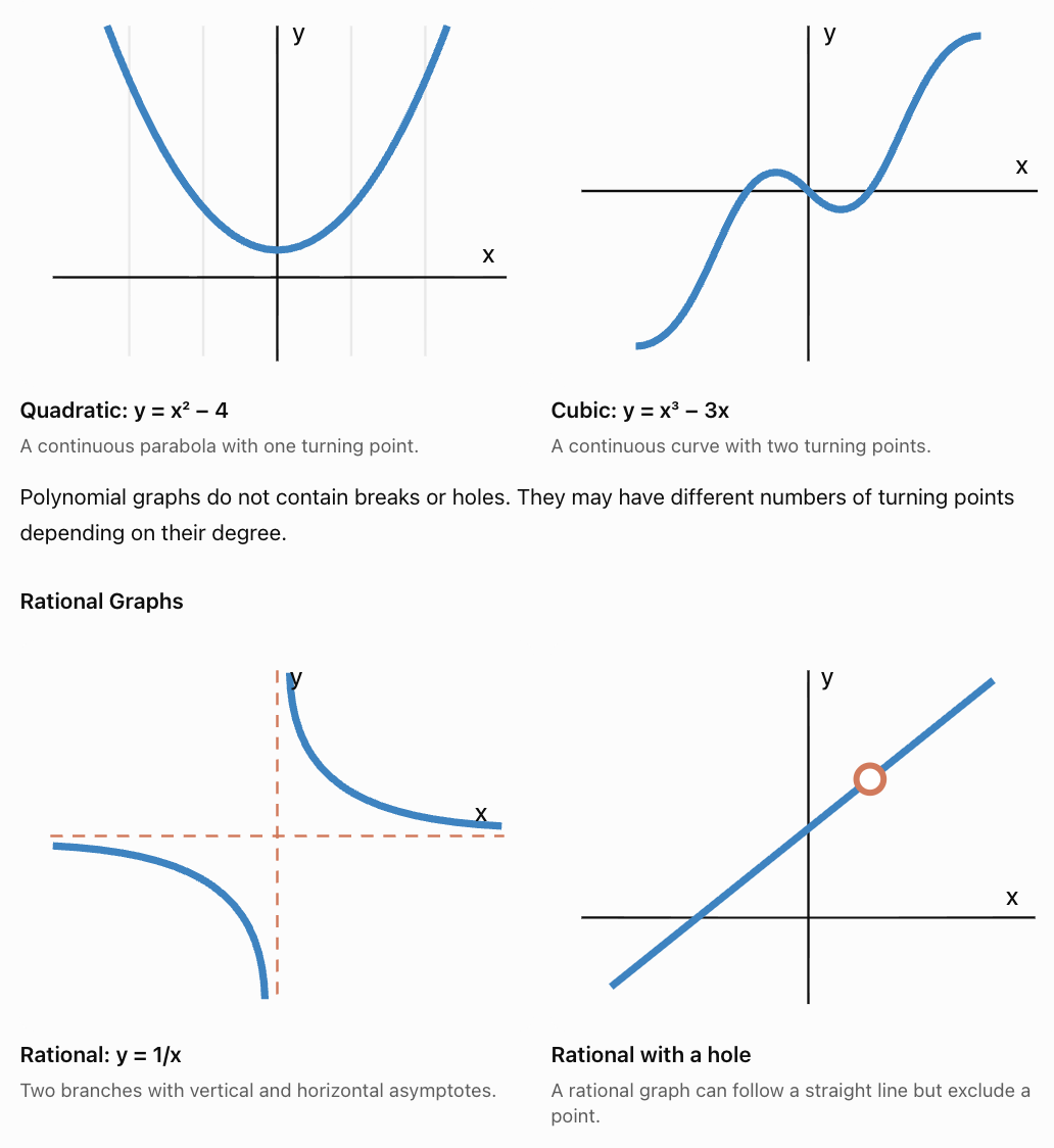
A graph with a vertical asymptote or a hole cannot be the graph of a polynomial function defined on all real numbers.

However, a smooth-looking graph alone does not prove that a function is polynomial. Some rational functions have no real denominator zeros and are continuous everywhere.

Comparing Domains

The domain of a function is the set of all input values for which the function is defined.

Domain of Polynomial Functions

Every polynomial function has the natural domain:

All real numbers.

In interval notation:

For example:

f(x) = x² − 5x + 6

We can substitute any real number for x without creating an undefined operation.

Therefore, the domain is all real numbers.

Domain of Rational Functions

For rational functions, we must exclude values that make the denominator zero.

Worked Example 1: Comparing Domains

Compare:

f(x) = x² − 9

g(x) = (x² − 9)/(x − 3)

Step 1: Find the polynomial domain.

f(x) is a polynomial.

Domain: all real numbers.

Step 2: Find the rational domain.

For g(x):

x − 3 = 0

x = 3

Therefore:

Domain: x ≠ 3.

Step 3: Simplify the rational function.

g(x) = (x − 3)(x + 3)/(x − 3)

g(x) = x + 3, where x ≠ 3.

Conclusion: Both functions have polynomial expressions associated with them, but the rational function has a missing point at (3, 6). The original polynomial f(x) = x² − 9 is defined at x = 3.

This example demonstrates that simplification does not eliminate original domain restrictions.

Comparing Ranges

The range of a function is the set of all possible output values.

Unlike the domain, the range often requires analyzing the graph, finding extrema, or solving an equation for x.

Range of Polynomial Functions

Different polynomial functions have different ranges.

For example:

f(x) = x² + 3

Since x² ≥ 0:

x² + 3 ≥ 3

Therefore:

Range: [3, ∞)

Range of Rational Functions

Rational functions may exclude certain output values because of asymptotes, holes, or other restrictions.

Consider:

g(x) = 1/x

The function can never equal zero because its numerator is 1.

Therefore:

Range: all real numbers except 0.

In interval notation:

Worked Example 2: Comparing Ranges

Compare:

f(x) = x²

g(x) = 1/(x² + 1)

Polynomial:

f(x) = x²

The minimum value occurs at x = 0.

f(0) = 0

As |x| increases, f(x) increases without bound.

Range:

[0, ∞)

Rational function:

g(x) = 1/(x² + 1)

Since x² ≥ 0:

x² + 1 ≥ 1

Therefore:

0 < 1/(x² + 1) ≤ 1

The maximum occurs at x = 0:

g(0) = 1

As |x| becomes very large, g(x) approaches zero but never reaches it.

Range:

(0, 1]

Conclusion: The polynomial has a minimum and no maximum, while the rational function has a maximum and approaches a lower bound it never reaches.

A Useful Warning About Horizontal Asymptotes

A horizontal asymptote is not automatically an excluded range value.

For example:

h(x) = (x² − 1)/(x² + 1)

has horizontal asymptote y = 1, and the graph never reaches 1.

But:

k(x) = (x² − 1)/(x² + 2)

also has horizontal asymptote y = 1 and never reaches it.

Other rational functions can cross their horizontal asymptotes. To determine the range, we must analyze the actual outputs rather than assuming the asymptote is excluded.

Comparing Intercepts

Both polynomial and rational functions can have x- and y-intercepts.

Polynomial Intercepts

For a polynomial function:

f(x) = P(x)

x-intercepts are found by solving:

P(x) = 0

The y-intercept is found by calculating:

f(0)

Every polynomial function has a y-intercept because its domain includes x = 0.

Rational Intercepts

For:

g(x) = P(x)/Q(x)

x-intercepts occur where:

P(x) = 0

provided Q(x) ≠ 0.

The y-intercept is g(0), provided Q(0) ≠ 0.

Worked Example 3: Comparing Intercepts

Compare:

f(x) = x² − 4

g(x) = (x² − 4)/(x + 2)

Polynomial:

Factor:

f(x) = (x − 2)(x + 2)

x-intercepts:

(−2, 0) and (2, 0)

y-intercept:

f(0) = −4

Therefore, (0, −4).

Rational function:

Factor:

g(x) = (x − 2)(x + 2)/(x + 2)

Simplify:

g(x) = x − 2, where x ≠ −2.

x-intercept:

(2, 0)

y-intercept:

g(0) = −2

Therefore, (0, −2).

Hole:

At x = −2, the simplified expression gives:

y = −2 − 2 = −4

Hole at (−2, −4).

Conclusion: The polynomial has two x-intercepts, while the rational function has one x-intercept and a hole.

Comparing End Behaviour

End behaviour describes what happens to a function as x approaches positive or negative infinity.

Polynomial End Behaviour

The degree and leading coefficient determine polynomial end behaviour.

For example:

f(x) = 2x⁴ − 3x² + 1

The leading term is 2x⁴.

Because the degree is even and the leading coefficient is positive, both ends of the graph rise.

Rational End Behaviour

Rational functions depend on the relative degrees of numerator and denominator.

For:

g(x) = P(x)/Q(x)

• If the numerator degree is smaller, the horizontal asymptote is y = 0.

• If the degrees are equal, the horizontal asymptote is the ratio of leading coefficients.

• If the numerator degree is exactly one greater, there is an oblique asymptote.

• If the numerator degree exceeds the denominator degree by two or more, there may be a higher-degree polynomial asymptote.

Worked Example 4: Comparing End Behaviour

Compare:

f(x) = x² + 2

g(x) = (x² + 2)/(x² + 1)

Polynomial:

As x approaches positive or negative infinity:

f(x) approaches positive infinity.

Rational function:

Both numerator and denominator have degree 2.

The ratio of leading coefficients is:

1/1 = 1

Therefore, the horizontal asymptote is y = 1.

We can rewrite:

g(x) = 1 + 1/(x² + 1)

As |x| increases, the second term approaches zero.

Therefore, g(x) approaches 1 from above.

Conclusion: The polynomial grows without bound, while the rational function approaches a finite value.

Comparing Continuity and Asymptotes

A polynomial function is continuous everywhere on the real number line.

This means that its graph can be drawn without lifting the pencil, and there are no holes, jumps, or vertical asymptotes.

Rational functions are continuous wherever their denominators are nonzero, but may be undefined at certain values.

Worked Example 5: A Rational Function with No Real Discontinuities

Consider:

g(x) = 1/(x² + 4)

The denominator is always positive because:

x² ≥ 0

Therefore:

x² + 4 ≥ 4

The denominator never equals zero.

So:

• Domain: all real numbers.

• No vertical asymptotes.

• No holes.

• Continuous everywhere.

• Horizontal asymptote: y = 0.

• Range: (0, 1/4].

This shows that not all rational functions have breaks in their graphs.

Similarities and Differences

Polynomial and rational functions have several important similarities.

Both can be evaluated by substitution, represented using tables and graphs, and analyzed using algebraic techniques. Both can have intercepts, turning points, increasing and decreasing intervals, and symmetry. Both can model real-world relationships.

Their most important differences concern domain restrictions, continuity, asymptotes, and end behaviour.

A polynomial's natural domain is always all real numbers, while a rational function may have excluded inputs. A polynomial is continuous everywhere, while a rational function may contain holes or vertical asymptotes.

Nevertheless, because every polynomial is also rational, these differences describe typical non-polynomial rational functions rather than an absolute separation between the two families.

Choosing Appropriate Mathematical Models

The choice between a polynomial and rational model depends on the relationship between the quantities.

A good mathematical model should:

• Represent the main pattern in the situation.

• Have a domain that makes sense in context.

• Produce reasonable predictions.

• Reflect important physical or mathematical restrictions.

• Be simple enough to interpret and use.

When to Use Polynomial Models

Polynomial models are often appropriate when a quantity changes according to sums of powers of another quantity.

Examples include:

• Projectile motion with constant gravitational acceleration.

• Area and volume calculations.

• Revenue and profit relationships.

• Curved trends that can be approximated using polynomial regression.

When to Use Rational Models

Rational models are often appropriate when a quantity involves division by a changing variable.

Examples include:

• Time required to travel a fixed distance.

• Average production cost.

• Concentration and dilution.

• Work rates.

• Inverse variation.

• Electrical relationships.

Real-World Application 1: Projectile Motion

Suppose a ball is thrown upward from a platform.

Its height in metres after t seconds is modelled by:

h(t) = −5t² + 20t + 2

This is a quadratic polynomial function.

Why is a polynomial model appropriate?

The equation describes vertical motion under constant gravitational acceleration, ignoring air resistance.

Find the maximum height.

The vertex occurs at:

t = −b/(2a)

Here:

a = −5, b = 20

Therefore:

t = −20/[2(−5)] = 2 seconds

Substitute:

h(2) = −5(2²) + 20(2) + 2

= −20 + 40 + 2

= 22

Maximum height: 22 m.

The mathematical polynomial is defined for all real t, but the physical model is meaningful only during the flight, from t = 0 until the ball reaches the ground.

Real-World Application 2: Average Production Cost

A company has a fixed cost of $800 and a variable cost of $12 per item.

The total cost is:

C(x) = 800 + 12x

This is a linear polynomial function.

However, the average cost per item is:

Simplify:

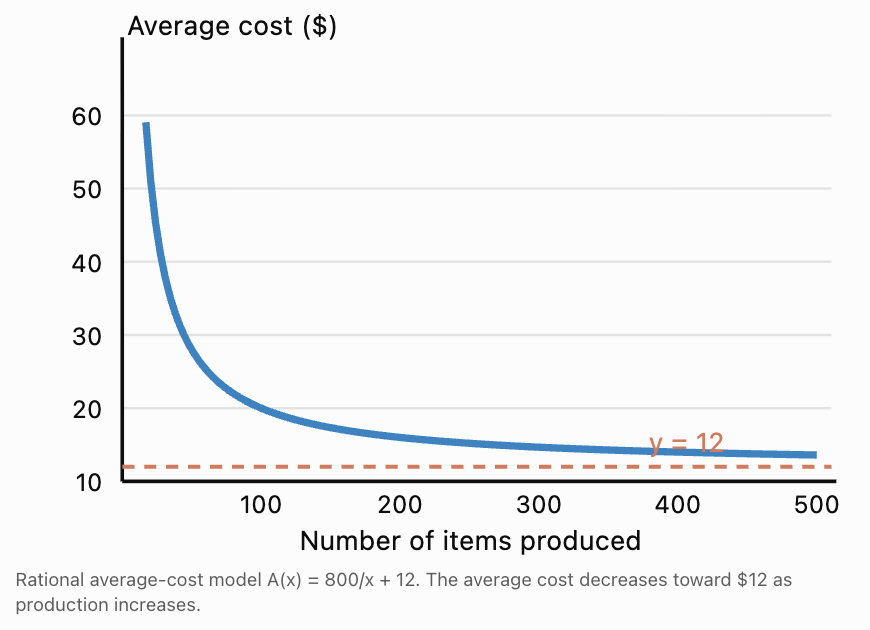
A(x) = 800/x + 12

This is a non-polynomial rational function.

As production increases, total cost increases linearly, but average cost decreases toward $12.

Why is a rational model appropriate for average cost?

Because average cost is calculated by dividing total cost by the number of items.

The rational function has a horizontal asymptote at y = 12, representing the variable cost per item.

Real-World Application 3: Travel Time

Suppose a car travels a fixed distance of 240 km.

The journey time is:

t(v) = 240/v

where v is speed in km/h.

This is a rational function.

Why not use a linear polynomial model?

Because doubling the speed halves the time, rather than reducing it by a constant amount.

The relationship is inverse variation, which is naturally represented by a rational function.

The physical domain is v greater than zero, with additional practical limits such as road speed restrictions.

Real-World Application 4: Comparing Two Models for the Same Situation

Suppose a business sells x items at $25 each and incurs a fixed cost of $500 plus $10 per item.

Revenue:

R(x) = 25x

Cost:

C(x) = 500 + 10x

Profit:

P(x) = R(x) − C(x)

P(x) = 15x − 500

This is a polynomial function.

However, profit per item is:

Simplify:

p(x) = 15 − 500/x

This is a rational function for x greater than zero.

The polynomial model describes total profit, while the rational model describes profit per item.

The same business situation may require different function families depending on the question being asked.

Evaluating the Reasonableness of a Model

A mathematical model may describe a pattern accurately over one interval but become unrealistic outside that interval.

For example, a polynomial model of population growth might eventually predict negative population values or implausibly rapid growth.

A rational model of average cost might approach a horizontal asymptote, but real production costs may change because of material shortages, capacity limits, or inflation.

Before using a model to make predictions, consider whether its assumptions remain reasonable over the intended domain.

Common Mistakes

Mistake 1: Assuming Polynomial and Rational Functions Are Completely Separate Categories

Every polynomial can be written as a rational function with denominator 1.

Therefore, all polynomial functions are rational functions, but not all rational functions are polynomial functions.

Mistake 2: Assuming Every Rational Function Has a Vertical Asymptote

The function f(x) = 1/(x² + 1) has no vertical asymptotes because its denominator never equals zero for real x.

Mistake 3: Forgetting Domain Restrictions After Simplifying

(x² − 4)/(x − 2) simplifies to x + 2, but x = 2 remains excluded.

The graph has a hole, unlike the complete polynomial line y = x + 2.

Mistake 4: Assuming Every Rational Function Has a Restricted Domain

Some rational functions, such as 1/(x² + 1), are defined for all real x.

Mistake 5: Assuming Horizontal Asymptotes Cannot Be Crossed

Horizontal asymptotes describe end behaviour. A rational graph may cross a horizontal asymptote at a finite input value.

Mistake 6: Confusing Domain and Range

Domain refers to permitted x-values.

Range refers to possible y-values.

For f(x) = 1/x, both exclude zero, but this is not true for every rational function.

Mistake 7: Choosing a Model Only Because Its Graph Looks Similar

A curve may resemble a polynomial or rational graph over a short interval.

The underlying relationship, domain, asymptotic behaviour, and physical meaning should also guide the model choice.

Key Terms

• Polynomial Function: A function expressed as a sum of terms containing nonnegative integer powers of a variable.

• Rational Function: A function expressed as the quotient of two polynomials, with a denominator that is not the zero polynomial.

• Degree: The highest exponent of a variable in a polynomial.

• Leading Coefficient: The coefficient of the highest-degree term.

• Domain: The set of all permitted input values.

• Range: The set of all possible output values.

• Continuous Function: A function whose graph has no breaks at points within its domain.

• Discontinuity: A point where a function is not continuous.

• Hole: A missing point caused by a removable discontinuity.

• Vertical Asymptote: A vertical line approached by a graph as function values increase or decrease without bound.

• Horizontal Asymptote: A horizontal line approached by a graph as x tends toward positive or negative infinity.

• Oblique Asymptote: A nonhorizontal straight line approached by a graph at infinity.

• x-Intercept: A point where a graph crosses or touches the x-axis.

• y-Intercept: A point where a graph intersects the y-axis.

• Turning Point: A point where a function changes from increasing to decreasing or vice versa.

• End Behaviour: The behaviour of a function as x approaches positive or negative infinity.

• Mathematical Model: A mathematical representation of a real-world relationship.

• Inverse Variation: A relationship in which one quantity is proportional to the reciprocal of another.

Key Takeaways

1. Polynomial functions contain sums of nonnegative integer powers of variables.

2. Rational functions are ratios of polynomials.

3. Every polynomial function is also a rational function, but not every rational function is a polynomial.

4. Polynomial functions have all real numbers as their natural domain.

5. Rational functions may have excluded values, holes, or vertical asymptotes.

6. Polynomial graphs are continuous and smooth everywhere.

7. Rational functions are continuous wherever their denominators are nonzero.

8. Both families can have intercepts, turning points, and useful real-world applications.

9. Polynomial end behaviour depends on degree and leading coefficient.

10. Rational end behaviour depends on the relative degrees of numerator and denominator.

11. Ranges must be determined from the actual outputs of the function.

12. Polynomial models are often suitable for trajectories, area, revenue, and profit.

13. Rational models are often suitable for rates, ratios, inverse variation, and average costs.

14. The most appropriate model depends on the mathematical relationship and the real-world context.

Check Your Understanding

Question 1: Classifying Functions

Classify each function as polynomial, rational but not polynomial, or neither.

a) f(x) = 3x² − 5x + 2

b) g(x) = 4/(x − 1)

c) h(x) = (x² + 1)/(x² + 4)

d) p(x) = √x + 3

Question 2: Comparing Domains

Find the natural domain of each function.

a) f(x) = x² − 16

b) g(x) = (x² − 16)/(x − 4)

Explain the difference.

Question 3: Comparing Ranges

Find the range of each function.

a) f(x) = x² + 2

b) g(x) = 1/(x² + 2)

Question 4: Comparing Intercepts

Find the x- and y-intercepts of:

a) f(x) = x² − 9

b) g(x) = (x² − 9)/(x + 3)

Question 5: Comparing Graph Features

Consider:

f(x) = x² + 1

g(x) = 1/(x² + 1)

For each function, identify:

a) Domain.

b) Range.

c) Any vertical asymptotes.

d) Horizontal asymptotes, if any.

Question 6: End Behaviour

Compare the end behaviour of:

f(x) = 2x³ − 4x

g(x) = (2x³ − 4x)/(x³ + 1)

Question 7: Choosing a Model

Choose whether a polynomial or non-polynomial rational function is more appropriate for each situation.

a) The height of a ball thrown upward under constant gravitational acceleration.

b) The time required to travel a fixed distance at different speeds.

c) The area of a square as its side length changes.

d) The average cost per item when production has a fixed cost and a constant variable cost.

Explain each choice.

Question 8: Real-World Modelling

A company has a fixed cost of $1,000 and a variable cost of $20 per item.

a) Write a polynomial function for total cost.

b) Write a rational function for average cost.

c) Calculate total and average cost for 100 items.

d) Identify and interpret the horizontal asymptote of the average-cost function.

Question 9: Challenge — Same Shape, Different Domain

Compare:

f(x) = x + 4

g(x) = (x² + 3x − 4)/(x − 1)

a) Simplify g(x).

b) Compare their domains.

c) Compare their ranges.

d) Explain how their graphs differ.

Fully Worked Answers

Answer 1: Classifying Functions

a) f(x) = 3x² − 5x + 2

This is a polynomial, and therefore also rational.

b) g(x) = 4/(x − 1)

This is rational but not polynomial because the variable appears in the denominator and the expression cannot simplify to a polynomial on all real numbers.

c) h(x) = (x² + 1)/(x² + 4)

This is rational but not polynomial.

d) p(x) = √x + 3

This is neither polynomial nor rational because √x is not a polynomial and cannot be expressed as a quotient of polynomials.

Answer 2: Comparing Domains

a) f(x) = x² − 16

Polynomial function.

Domain: all real numbers.

b) g(x) = (x² − 16)/(x − 4)

Set the denominator equal to zero:

x − 4 = 0

x = 4

Therefore, x ≠ 4.

Factoring gives:

g(x) = (x − 4)(x + 4)/(x − 4)

g(x) = x + 4, where x ≠ 4.

The rational graph has a hole at (4, 8).

Conclusion: The polynomial is defined everywhere, while the rational function excludes x = 4.

Answer 3: Comparing Ranges

a) f(x) = x² + 2

Since x² ≥ 0:

x² + 2 ≥ 2

Minimum output = 2.

Range:

[2, ∞)

b) g(x) = 1/(x² + 2)

Since x² ≥ 0:

x² + 2 ≥ 2

Therefore:

0 < g(x) ≤ 1/2

Range:

(0, 1/2]

Answer 4: Comparing Intercepts

a) f(x) = x² − 9

x-intercepts:

x² − 9 = 0

(x − 3)(x + 3) = 0

x = −3 or x = 3

Therefore:

(−3, 0) and (3, 0).

y-intercept:

f(0) = −9

Therefore:

(0, −9).

b) g(x) = (x² − 9)/(x + 3)

Factor:

g(x) = (x − 3)(x + 3)/(x + 3)

Simplify:

g(x) = x − 3, where x ≠ −3.

x-intercept:

x − 3 = 0

x = 3

Therefore:

(3, 0).

y-intercept:

g(0) = −3

Therefore:

(0, −3).

The graph also has a hole at (−3, −6).

Answer 5: Comparing Graph Features

Polynomial: f(x) = x² + 1

Domain: all real numbers.

Since x² ≥ 0:

f(x) ≥ 1

Range: [1, ∞).

Vertical asymptotes: none.

Horizontal asymptotes: none.

Rational: g(x) = 1/(x² + 1)

Domain: all real numbers, because x² + 1 is always positive.

Maximum output occurs at x = 0:

g(0) = 1

The function approaches zero as |x| increases but never equals zero.

Range: (0, 1].

Vertical asymptotes: none.

Horizontal asymptote: y = 0.

Answer 6: End Behaviour

Polynomial:

f(x) = 2x³ − 4x

The leading term is 2x³.

As x approaches positive infinity, f(x) approaches positive infinity.

As x approaches negative infinity, f(x) approaches negative infinity.

Rational function:

g(x) = (2x³ − 4x)/(x³ + 1)

Both polynomials have degree 3.

The leading coefficient ratio is:

2/1 = 2

Therefore, the horizontal asymptote is y = 2.

As x approaches positive or negative infinity, g(x) approaches 2.

Answer 7: Choosing a Model

a) Projectile height: Polynomial.

Under constant gravitational acceleration, height is modelled by a quadratic function of time.

b) Travel time: Rational.

Time = Distance / Speed.

c) Area of a square: Polynomial.

A(s) = s².

d) Average production cost: Rational.

Average cost = Total cost / Number of items.

When total cost includes fixed and variable components, the average-cost function typically contains a term proportional to 1/x.

Answer 8: Real-World Modelling

a) Total cost

C(x) = 1000 + 20x

This is a linear polynomial function.

b) Average cost

A(x) = (1000 + 20x)/x

Simplify:

A(x) = 1000/x + 20

For the application, x must be a positive whole number.

c) At 100 items

Total cost:

C(100) = 1000 + 20(100)

= $3,000

Average cost:

A(100) = 3000/100

= $30 per item.

d) Horizontal asymptote

As x becomes large, 1000/x approaches zero.

Therefore:

y = 20.

This represents the variable production cost per item.

The average cost approaches $20 as the fixed cost is spread across more items.

Answer 9: Challenge

Given:

f(x) = x + 4

g(x) = (x² + 3x − 4)/(x − 1)

a) Simplify g(x).

Factor the numerator:

x² + 3x − 4 = (x + 4)(x − 1)

Therefore:

g(x) = (x + 4)(x − 1)/(x − 1)

g(x) = x + 4, where x ≠ 1.

b) Compare domains.

f(x): all real numbers.

g(x): all real numbers except x = 1.

c) Compare ranges.

f(x) = x + 4 has range all real numbers.

For g(x), the excluded input x = 1 would give the output:

1 + 4 = 5

Because x + 4 is one-to-one, no other input gives y = 5.

Therefore:

Range of g(x): all real numbers except 5.

d) Compare graphs.

Both graphs follow the line y = x + 4.

However, g(x) has a hole at (1, 5), while f(x) includes that point.

This completes Comparing Polynomial and Rational Functions, covering the characteristics of both families, their graphs, domains and ranges, similarities and differences, and the selection of appropriate mathematical models for real-world situations.