Applications and Mathematical Modelling

 

 

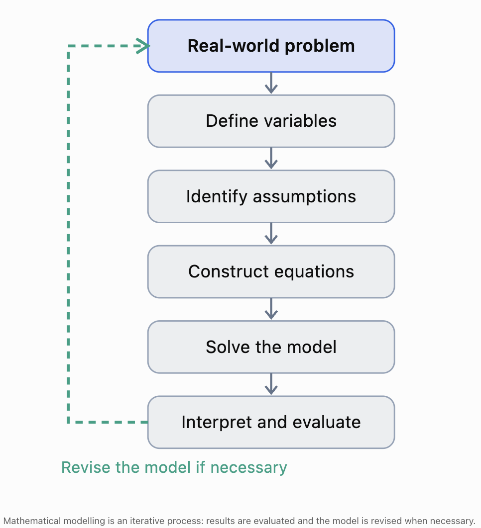
Understanding the stages

Real-world problem: Identify what needs to be investigated or decided.

Define variables: Represent unknown quantities with suitable symbols.

Identify assumptions: Decide which features of reality can be simplified.

Construct equations: Translate the available information into mathematical relationships.

Solve the model: Use algebraic, graphical, numerical, or technological methods.

Interpret and evaluate: Explain the results, check them against reality, and determine whether the model should be improved.

The final stage is particularly important.

A model may produce a mathematically correct solution that is unrealistic or unsuitable for the original problem.

Variables, Parameters, and Constraints

Three important components of mathematical models are variables, parameters, and constraints.

Variables

A variable represents a quantity that can change or an unknown value.

Examples:

x = number of products sold

t = time, in seconds

v = velocity, in m/s

Parameters

A parameter is a value that defines a particular model.

For example:

C = 500 + 8x

Here:

• C is total cost.

• x is production quantity.

• 500 is the fixed cost.

• 8 is the variable cost per unit.

The numbers 500 and 8 are parameters of the cost model.

They may change if the business conditions change.

Constraints

A constraint restricts which solutions are acceptable.

For example, if x represents the number of products manufactured:

x ≥ 0

If products must be complete units:

x must be a whole number.

If a factory can produce at most 300 units:

x ≤ 300

Constraints are important because a mathematical system may produce solutions that are not realistic.

Example

A factory model produces:

x = 125.5

y = 74.5

These values may satisfy the equations.

However, if x and y represent complete manufactured products, the solution is not physically possible as an exact production plan.

The model may need to be adjusted or solved using integer constraints.

Identifying Assumptions in Mathematical Models

An assumption is a condition accepted as true for the purpose of constructing or using a model.

Assumptions simplify complex situations.

For example, a model of vehicle motion may assume that speed remains constant.

A business model may assume that selling price does not change.

A mixture model may assume that volumes are additive.

Common assumptions

Why assumptions matter

Assumptions make mathematical modelling manageable, but they also limit how accurately a model represents reality.

For example, consider:

C = 1000 + 5x

This model assumes that fixed costs remain $1,000 and variable costs remain $5 per unit.

However, producing more units might require a second factory shift, additional equipment, or overtime pay.

The original model may no longer be accurate beyond a certain production level.

A good mathematical conclusion should explain the assumptions on which the result depends.

Worked Example: Modelling a School Event

A school sells adult and student tickets for a performance.

Adult tickets cost $15.

Student tickets cost $10.

A total of 200 tickets are sold.

Total revenue is $2,400.

Determine the number of adult and student tickets sold.

Step 1: Identify the unknowns

Let:

a = number of adult tickets

s = number of student tickets

Step 2: Identify assumptions

Assume:

• Every ticket sold is either an adult or student ticket.

• Adult tickets all cost $15.

• Student tickets all cost $10.

• There are no refunds or discounts.

• Revenue includes only ticket sales.

Step 3: Construct the equations

Total tickets:

a + s = 200

Total revenue:

15a + 10s = 2400

Step 4: Solve by elimination

Multiply the first equation by 10:

10a + 10s = 2000

Subtract from the revenue equation:

5a = 400

a = 80

Then:

s = 200 − 80

s = 120

Step 5: Interpret

80 adult tickets were sold.

120 student tickets were sold.

Step 6: Verify

Total tickets:

80 + 120 = 200

Revenue:

15(80) + 10(120)

= 1200 + 1200

= $2400

Answer: 80 adult tickets and 120 student tickets.

Step 7: Evaluate the model

The result is reasonable because:

• Both quantities are nonnegative.

• Both quantities are whole numbers.

• The total number of tickets is correct.

• The revenue matches the recorded amount.

However, if discounted tickets or complimentary admissions were included, the model might need additional variables.

Worked Example: Modelling Production and Resource Use

A small factory manufactures tables and chairs.

Each table requires:

• 5 hours of labour.

• 4 units of wood.

Each chair requires:

• 2 hours of labour.

• 3 units of wood.

During one production period, the factory uses:

• 90 labour-hours.

• 80 units of wood.

Determine the number of tables and chairs produced.

Step 1: Define variables

t = number of tables

c = number of chairs

Step 2: Construct the equations

Labour:

5t + 2c = 90

Wood:

4t + 3c = 80

Step 3: Solve by elimination

Multiply the first equation by 3:

15t + 6c = 270

Multiply the second equation by 2:

8t + 6c = 160

Subtract:

7t = 110

t = 110/7 ≈ 15.714

Substitute into the first equation:

5(110/7) + 2c = 90

550/7 + 2c = 630/7

2c = 80/7

c = 40/7 ≈ 5.714

Step 4: Interpret

The system produces:

t ≈ 15.714 tables

c ≈ 5.714 chairs

These quantities are mathematically valid but not realistic for complete furniture products.

Step 5: Evaluate

The model assumes that both recorded resource totals were used entirely to manufacture complete tables and chairs.

Because the solution contains fractional quantities, the recorded totals and assumptions cannot all describe a production plan consisting only of complete items.

Step 6: Improve the model

Possible explanations include:

• Some materials were wasted.

• Some labour-hours were used for other activities.

• Resource measurements were rounded.

• Production requirements vary between individual products.

If the factory is planning future production rather than reconstructing past production, it may be more appropriate to use inequalities:

5t + 2c ≤ 90

4t + 3c ≤ 80

t ≥ 0, c ≥ 0

with t and c restricted to whole numbers.

This changes the task from solving an exact system to finding a feasible production plan.

Important lesson: A mathematical model may reveal that the original assumptions are too restrictive or that the data are inconsistent with the intended interpretation.

Improving a Model with Realistic Data

Consider a revised production example.

A factory manufactures tables and chairs.

Each table requires 5 labour-hours and 4 units of wood.

Each chair requires 2 labour-hours and 3 units of wood.

The factory uses:

• 70 labour-hours.

• 60 units of wood.

The model becomes:

5t + 2c = 70

4t + 3c = 60

Multiply the first equation by 3:

15t + 6c = 210

Multiply the second equation by 2:

8t + 6c = 120

Subtract:

7t = 90

t = 90/7

This still produces a fractional solution.

This tells us that changing the totals does not automatically produce a feasible integer solution.

A better approach is to choose a feasible production plan and calculate its resource requirements.

Suppose the factory produces:

t = 10 tables

c = 15 chairs

Then:

Labour:

5(10) + 2(15) = 80 hours

Wood:

4(10) + 3(15) = 85 units

A consistent model is therefore:

5t + 2c = 80

4t + 3c = 85

Solving this system gives:

t = 10, c = 15

This illustrates how mathematical models can be checked against feasible real-world scenarios.

Worked Example: Modelling Travel and Motion

Two vehicles leave the same location at the same time and travel in opposite directions.

After 4 hours, they are 320 km apart.

The faster vehicle travels 20 km/h faster than the slower vehicle.

Find their speeds.

Step 1: Define variables

x = speed of slower vehicle, in km/h

y = speed of faster vehicle, in km/h

Step 2: Identify assumptions

Assume:

• Both vehicles maintain constant speeds.

• They travel in opposite directions along a straight route.

• They begin at the same time.

• Neither vehicle stops.

Step 3: Construct equations

Distance = speed × time

Combined separation:

4x + 4y = 320

Simplify:

x + y = 80

Speed difference:

y − x = 20

Step 4: Solve

Add the equations:

2y = 100

y = 50

Then:

x = 30

Step 5: Interpret

Slower vehicle = 30 km/h

Faster vehicle = 50 km/h

Step 6: Verify

Distances:

30(4) = 120 km

50(4) = 200 km

Combined separation:

120 + 200 = 320 km

Speed difference:

50 − 30 = 20 km/h

Answer: The vehicles travel at 30 km/h and 50 km/h.

Step 7: Evaluate

The model is appropriate if the vehicles travel at approximately constant speeds.

If the vehicles accelerate, stop, or follow curved routes, a more complex model may be required.

Worked Example: Modelling a Chemical Mixture

A laboratory needs 500 mL of a 20% solution.

It has:

• A 10% solution.

• A 30% solution.

Determine the volume of each solution required.

Step 1: Define variables

x = volume of 10% solution, in mL

y = volume of 30% solution, in mL

Step 2: Identify assumptions

Assume:

• The concentration percentages use the same definition.

• Volumes are additive.

• No solute is lost during mixing.

• The solutions are mixed completely.

Step 3: Construct equations

Total volume:

x + y = 500

Solute-equivalent volume:

0.10x + 0.30y = 0.20(500)

Simplify:

0.10x + 0.30y = 100

Step 4: Solve

From the first equation:

x = 500 − y

Substitute:

0.10(500 − y) + 0.30y = 100

50 − 0.10y + 0.30y = 100

0.20y = 50

y = 250

Then:

x = 250

Step 5: Verify

Total volume:

250 + 250 = 500 mL

Solute-equivalent volume:

0.10(250) + 0.30(250)

= 25 + 75

= 100 mL

Final concentration:

100/500 × 100% = 20%

Answer: 250 mL of each solution.

Step 6: Evaluate

The result is valid under the stated assumptions.

For precise laboratory work, volume changes during mixing and the definition of concentration may need to be considered.

Worked Example: Comparing Two Cost Models

A business is considering two equipment rental plans.

Plan A:

$500 fixed charge plus $20 per hour.

Plan B:

$200 fixed charge plus $35 per hour.

At how many hours do the plans cost the same?

Step 1: Define variables

h = number of rental hours

C = total rental cost, in dollars

Step 2: Construct equations

Plan A:

C = 500 + 20h

Plan B:

C = 200 + 35h

Step 3: Solve

500 + 20h = 200 + 35h

300 = 15h

h = 20

Step 4: Calculate the cost

Plan A:

C = 500 + 20(20) = $900

Plan B:

C = 200 + 35(20) = $900

Answer: Both plans cost $900 for 20 hours of rental.

Step 5: Interpret

For fewer than 20 hours, Plan B is cheaper.

For more than 20 hours, Plan A is cheaper.

At exactly 20 hours, the costs are equal.

Step 6: Evaluate

The model assumes that both plans charge according to the stated rates.

It ignores taxes, discounts, minimum rental periods, and additional fees.

These factors could affect the actual cost comparison.

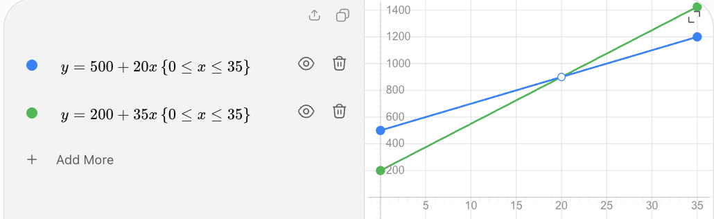
The two cost models intersect at 20 hours and $900. The graph represents the simplified pricing assumptions.

Choosing an Appropriate Method to Solve a Model

Different mathematical models may be easier to solve using different methods.

Substitution

Substitution is useful when one variable is already isolated or can be isolated easily.

Example:

x + y = 50

y = 2x + 5

Substitute the second equation into the first.

Elimination

Elimination is useful when coefficients can be made equal or opposite.

Example:

3x + 2y = 40

5x − 2y = 24

Adding the equations eliminates y.

Graphing

Graphing is useful when the model involves two variables and the intersection has a meaningful interpretation.

For example, cost and revenue models can be graphed to identify a break-even point.

Matrix methods

Matrix methods are useful for larger systems involving three or more variables.

A system such as:

2x + y + z = 12

x + 3y + 2z = 17

3x + 2y + 4z = 25

can be represented in matrix form:

A𝐱 = 𝐛

where A contains the coefficients, 𝐱 contains the unknowns, and 𝐛 contains the constants.

Technology

Graphing calculators, spreadsheets, and mathematical software are useful when:

• Systems contain many variables.

• Coefficients are complicated.

• Several scenarios must be compared.

• Models need to be updated frequently.

• Experimental data must be analysed.

However, technology does not replace the need to understand the assumptions and meaning of a model.

Modelling with Three Variables

Some situations require three or more unknown quantities.

Worked Example: A School Fundraising Sale

A school sells three products:

• Notebooks for $5.

• Water bottles for $10.

• T-shirts for $15.

A total of 100 products are sold.

Total revenue is $900.

The number of notebooks sold is twice the number of T-shirts sold.

Find the quantity of each product.

Step 1: Define variables

n = number of notebooks

w = number of water bottles

t = number of T-shirts

Step 2: Construct equations

Total quantity:

n + w + t = 100

Total revenue:

5n + 10w + 15t = 900

Quantity relationship:

n = 2t

Step 3: Substitute

From the third equation:

n = 2t

Substitute into the quantity equation:

2t + w + t = 100

w + 3t = 100

Therefore:

w = 100 − 3t

Substitute into the revenue equation:

5(2t) + 10(100 − 3t) + 15t = 900

10t + 1000 − 30t + 15t = 900

1000 − 5t = 900

−5t = −100

t = 20

Then:

n = 2(20) = 40

w = 100 − 3(20) = 40

Step 4: Interpret

Notebooks: 40

Water bottles: 40

T-shirts: 20

Step 5: Verify

Total quantity:

40 + 40 + 20 = 100

Revenue:

5(40) + 10(40) + 15(20)

= 200 + 400 + 300

= $900

Quantity relationship:

40 = 2(20)

Answer: 40 notebooks, 40 water bottles, and 20 T-shirts.

Step 6: Evaluate

The model assumes constant prices and that the revenue comes only from these three products.

The result is reasonable because all quantities are nonnegative whole numbers and satisfy every condition.

Models with No Solution or Infinitely Many Solutions

Not every system has a unique solution.

No solution

Consider:

x + y = 100

x + y = 120

These equations cannot both be true.

The model is inconsistent.

In a real-world situation, this may indicate incorrect data, incompatible measurements, or an unsuitable assumption.

Infinitely many solutions

Consider:

x + y = 100

2x + 2y = 200

The second equation provides no new information.

Many pairs of values satisfy both equations.

The model is underdetermined.

Additional independent information is needed to determine a unique solution.

Why this matters

A mathematical model may fail to determine a unique answer because the available information is insufficient.

Recognising this limitation is an important part of modelling.

Evaluating How Well a Model Represents Reality

A mathematical model should be evaluated using more than mathematical correctness.

Accuracy

Does the model reproduce observed measurements?

For example, if a model predicts 100 units sold but the business records only 70, the model may need revision.

Reasonableness

Are the calculated values realistic?

A model predicting negative production quantities is usually inappropriate for a physical manufacturing situation.

Assumptions

Are the simplifying assumptions valid?

A constant-speed model may be unsuitable for a vehicle that accelerates and brakes frequently.

Sensitivity

How much do the results change when the inputs change?

If a small change in measurement produces a large change in the solution, the model may be sensitive to uncertainty.

Range of validity

Does the model remain accurate over the range where it is being used?

A linear cost model may be accurate for 100–500 units but inaccurate for 10,000 units.

Predictive usefulness

Can the model make reliable predictions about situations not used to construct it?

A model that matches past data perfectly may still perform poorly when predicting future outcomes.

Practical constraints

Does the solution satisfy real-world restrictions?

Examples include:

• Production capacity.

• Available resources.

• Nonnegative quantities.

• Whole-number requirements.

• Maximum speed or force limits.

• Financial budgets.

Sensitivity Analysis

Sensitivity analysis investigates how changes in the assumptions or parameters affect the solution.

Consider the equipment rental models:

Plan A:

Cₐ = 500 + 20h

Plan B:

Cᵦ = 200 + 35h

The equal-cost point is 20 hours.

Now suppose Plan B increases its hourly rate from $35 to $40.

The revised equation is:

Cᵦ = 200 + 40h

Set the costs equal:

500 + 20h = 200 + 40h

300 = 20h

h = 15

The equal-cost point changes from 20 hours to 15 hours.

Interpretation

Increasing Plan B's hourly rate makes Plan A more competitive at a lower rental duration.

This illustrates how a change in one model parameter can affect the final decision.

Comparison

The model can be used to investigate different pricing scenarios before making a decision.

Model Validation and Experimental Data

A model is validated by comparing its predictions with observations or independent data.

Suppose a scientist models the position of an object using:

s = 4t + 2

where:

• s = position, in metres.

• t = time, in seconds.

The model predicts:

Suppose the actual measurements are:

The measurements are close to the predictions.

This suggests that the linear model may be appropriate over the observed time interval.

However, additional measurements would be needed to determine whether the model remains accurate over longer periods.

Residuals

A residual is the difference between an observed value and a predicted value.

Residual = observed value − predicted value

At t = 2 s:

Residual = 10.2 − 10

Residual = +0.2 m

At t = 3 s:

Residual = 13.8 − 14

Residual = −0.2 m

Small residuals suggest that the model closely matches the measurements.

However, the pattern of residuals is also important.

A systematic pattern may indicate that the model is missing an important relationship.

Improving Mathematical Models

A model can be improved by:

• Collecting more accurate data.

• Adding relevant variables.

• Revising unrealistic assumptions.

• Including important constraints.

• Using a nonlinear relationship when necessary.

• Comparing predictions with independent observations.

• Considering measurement uncertainty.

• Testing the model over different conditions.

Example: Improving a Motion Model

Initial model:

s = vt + s₀

This assumes constant velocity.

If an object accelerates at a constant rate, a better model may be:

s = s₀ + ut + ½at²

where:

• s₀ = initial position.

• u = initial velocity.

• a = constant acceleration.

• t = time.

The improved model includes acceleration and can represent a wider range of motion situations.

However, it also introduces additional parameters that must be determined from measurements.

This illustrates a common modelling trade-off:

More detailed models may represent reality more accurately, but they often require more information and more complex mathematics.

Communicating Mathematical Modelling Conclusions

A strong modelling conclusion should include:

1. The mathematical result.

2. The meaning of the result in context.

3. Appropriate units.

4. Verification or supporting evidence.

5. Relevant assumptions.

6. Limitations and possible improvements.

Example: Weak conclusion

x = 20

Improved conclusion

The two equipment rental plans have the same cost at 20 hours.

Strong conclusion

The two rental plans each cost $900 at 20 hours. Plan B is cheaper for shorter rental periods, while Plan A is cheaper for longer periods. This conclusion assumes the stated fixed and hourly charges remain unchanged and that there are no additional fees. The business should confirm these conditions before selecting a plan.

The final version provides information that can support a practical decision.

Common Mistakes

Starting calculations before defining variables

Clearly identify every unknown quantity and its units.

Constructing equations that do not match the situation

Check that each equation accurately represents the given information.

Ignoring assumptions

A model may be inappropriate if its assumptions do not reflect reality.

Confusing variables and parameters

Variables represent unknown or changing quantities, while parameters define particular relationships in the model.

Ignoring constraints

A mathematically correct answer may violate production limits or physical restrictions.

Assuming every system has one solution

Some models are inconsistent or underdetermined.

Rounding too early

Premature rounding may introduce significant errors.

Using inappropriate units

All quantities must use consistent units.

Accepting fractional quantities when whole numbers are required

Production counts and population counts often require integer solutions.

Failing to verify the result

Substitute the calculated values into the original equations.

Assuming a model is exact

Real-world models involve simplifications and uncertainty.

Failing to evaluate predictions

Compare model predictions with observations whenever possible.

Providing answers without interpretation

Explain what the solution means and how it can be used.

Key Terms

• Mathematical modelling: Representing real-world situations using mathematical relationships.

• Mathematical model: A simplified mathematical representation of a situation.

• Variable: A symbol representing an unknown or changing quantity.

• Parameter: A value that defines a particular model.

• Constraint: A restriction on possible solutions.

• Assumption: A condition accepted as true for the purpose of constructing a model.

• System of equations: Two or more equations solved simultaneously.

• Linear model: A model based on linear relationships.

• Nonlinear model: A model containing relationships that are not linear.

• Substitution: Replacing a variable with an equivalent expression.

• Elimination: Combining equations to remove a variable.

• Graphical solution: A solution found or represented using graphs.

• Matrix method: A method of representing and solving systems using matrices.

• Unique solution: Exactly one set of values satisfying a system.

• Inconsistent system: A system with no solution.

• Underdetermined model: A model with insufficient independent information to determine a unique solution.

• Verification: Checking that a solution satisfies the original equations.

• Validation: Comparing a model's predictions with real-world evidence.

• Residual: The difference between an observed value and a predicted value.

• Sensitivity analysis: Investigating how changes in inputs affect model outputs.

• Range of validity: The conditions under which a model is considered appropriate.

• Predictive accuracy: How closely model predictions match actual outcomes.

• Feasible solution: A solution satisfying all mathematical and practical constraints.

• Model refinement: Improving a model by adjusting its assumptions, relationships, or parameters.

Key Takeaways

• Mathematical modelling connects real-world situations with mathematical relationships.

• Systems of equations are useful when several unknown quantities are connected.

• Variables, parameters, assumptions, and constraints are essential components of models.

• A modelling process involves defining, constructing, solving, interpreting, evaluating, and revising.

• Substitution, elimination, graphing, matrices, and technology can be used to solve systems.

• Mathematical solutions must be interpreted in the original context.

• A mathematically correct result may not be practically feasible.

• Models may have unique solutions, no solutions, or infinitely many solutions.

• Assumptions determine when a model is appropriate.

• Sensitivity analysis reveals how changes in inputs affect results.

• Validation compares predictions with observed data.

• Models should be revised when evidence shows that their predictions are unreliable.

Check Your Understanding

Recall and Understanding

1. Define mathematical modelling and explain why it is useful.

2. Explain the difference between a variable, parameter, and constraint.

3. Why are assumptions necessary when constructing mathematical models?

4. Explain the difference between verification and validation.

5. Why might a mathematically correct solution be unsuitable in a real-world situation?

Constructing and Solving Models

6. A school sells adult tickets for $12 and student tickets for $8.

A total of 150 tickets are sold, generating $1,500.

Construct a system and determine the number of each ticket type.

7. A factory produces two products.

Product A requires 3 labour-hours.

Product B requires 5 labour-hours.

The factory produces 100 units using 380 labour-hours.

Find the quantity of each product.

8. Two vehicles travel in opposite directions.

After 3 hours, they are 210 km apart.

One vehicle travels 10 km/h faster than the other.

Find their speeds.

9. A laboratory needs 600 mL of a 25% solution.

It has a 10% solution and a 40% solution.

Assuming compatible concentrations and additive volumes, determine the required volumes.

10. Two service plans have costs:

Plan A: C = 300 + 15x

Plan B: C = 100 + 25x

Find the value of x at which the plans cost the same.

Three-Variable Models

11. A school sells notebooks, pens, and folders.

Notebooks cost $5, pens cost $2, and folders cost $8.

A total of 100 items are sold for $500.

The number of notebooks equals the number of folders.

Find the number of each item.

12. A factory manufactures three products.

The total number of products is 120.

Product A requires 2 hours, Product B requires 3 hours, and Product C requires 4 hours.

The total labour time is 360 hours.

The number of Product A units equals the number of Product C units.

Determine whether the system has a unique solution.

Model Evaluation

13. A production model gives:

x = 25.5

y = 14.5

Explain why these values might be unsuitable and suggest an improvement.

14. A motion model assumes constant velocity.

Explain how the model might be improved if the object accelerates.

15. A business cost model predicts $2,000 in total costs, but actual costs are $2,450.

Calculate the residual using observed minus predicted, and explain what it indicates.

16. A model produces:

x + y = 100

2x + 2y = 200

Explain why the system cannot determine unique values.

17. A model produces:

x + y = 100

x + y = 120

Explain what this result indicates about the model or data.

18. A company uses the model:

C = 1000 + 5x

Explain why the model may become inaccurate at very high production levels.

19. A rental plan comparison produces an equal-cost point of 18.6 hours.

Explain how this result should be interpreted if rental time is charged in complete hours.

20. A scientist constructs a model using two experimental measurements.

The model fits both measurements exactly.

Explain why this does not necessarily mean that the model is reliable.

Answers to Check Your Understanding

1. Mathematical modelling

Mathematical modelling is the process of representing real-world situations using mathematical relationships.

It is useful for analysing situations, determining unknown quantities, making predictions, and supporting decisions.

2. Variables, parameters, and constraints

A variable represents an unknown or changing quantity.

A parameter is a value that defines a particular model.

A constraint restricts possible solutions.

For example:

C = 500 + 8x

x is a variable.

500 and 8 are parameters.

A constraint might be:

0 ≤ x ≤ 300

3. Assumptions

Assumptions simplify complex situations so they can be represented mathematically.

However, assumptions must be reasonable because they affect the accuracy and usefulness of the model.

4. Verification and validation

Verification checks whether a solution satisfies the mathematical equations.

Validation checks whether the model represents real-world observations accurately enough for its intended purpose.

5. Unsuitable mathematical solutions

A solution may violate real-world restrictions.

For example, a production model might produce a negative quantity or a fractional number of complete products.

Such values may satisfy the equations but not represent feasible outcomes.

6. Ticket sales

Let:

a = adult tickets

s = student tickets

Equations:

a + s = 150

12a + 8s = 1500

Multiply the first equation by 8:

8a + 8s = 1200

Subtract:

4a = 300

a = 75

Then:

s = 75

Answer: 75 adult tickets and 75 student tickets.

Verification:

75 + 75 = 150

12(75) + 8(75) = $1500

7. Factory production

Let:

x = Product A units

y = Product B units

Equations:

x + y = 100

3x + 5y = 380

Multiply the first equation by 3:

3x + 3y = 300

Subtract:

2y = 80

y = 40

Then:

x = 60

Answer: 60 units of Product A and 40 units of Product B.

8. Vehicle speeds

Let:

x = slower speed

y = faster speed

Distance:

3x + 3y = 210

x + y = 70

Speed difference:

y − x = 10

Add:

2y = 80

y = 40

x = 30

Answer: 30 km/h and 40 km/h.

9. Solution mixture

Let:

x = volume of 10% solution

y = volume of 40% solution

Equations:

x + y = 600

0.10x + 0.40y = 150

Substitute x = 600 − y:

60 − 0.10y + 0.40y = 150

0.30y = 90

y = 300

x = 300

Answer: 300 mL of each solution.

10. Service plans

Set costs equal:

300 + 15x = 100 + 25x

200 = 10x

x = 20

Cost:

300 + 15(20) = 600

Answer: The plans cost the same at x = 20, with a cost of $600.

11. Three-product sales

Let:

n = notebooks

p = pens

f = folders

Equations:

n + p + f = 100

5n + 2p + 8f = 500

n = f

Substitute f = n:

2n + p = 100

p = 100 − 2n

Revenue:

5n + 2(100 − 2n) + 8n = 500

5n + 200 − 4n + 8n = 500

9n = 300

n = 100/3

Therefore:

f = 100/3

p = 100 − 200/3 = 100/3

Mathematical solution: n = p = f = 100/3.

However, the quantities represent complete items.

Therefore, the system has no feasible whole-number solution.

The sales information may contain an error or may require an additional assumption.

12. Three-variable production

Let:

a = Product A units

b = Product B units

c = Product C units

Equations:

a + b + c = 120

2a + 3b + 4c = 360

a = c

Substitute c = a:

2a + b = 120

2a + 3b + 4a = 360

6a + 3b = 360

Divide by 3:

2a + b = 120

The equations are dependent.

Answer: The system does not have a unique solution.

Possible solutions satisfy:

a = c = t

b = 120 − 2t

For nonnegative whole-number quantities:

t can be any integer from 0 to 60.

Additional independent information is needed to determine a unique production plan.

13. Fractional production quantities

The model produces:

x = 25.5

y = 14.5

If x and y represent complete products, fractional values are not feasible.

The model could be improved by including whole-number constraints or revising assumptions about resource use.

14. Accelerating motion

A constant-velocity model such as:

s = vt + s₀

may not be appropriate when velocity changes.

For constant acceleration, use:

s = s₀ + ut + ½at²

This model includes acceleration.

15. Cost residual

Observed cost = $2450

Predicted cost = $2000

Residual:

2450 − 2000 = 450

Answer: +$450.

The model underestimates the actual cost by $450.

The discrepancy may indicate missing costs, incorrect parameters, or changing business conditions.

16. Dependent equations

The second equation is twice the first.

Therefore, it provides no new information.

The system has infinitely many solutions.

An additional independent equation is needed to determine unique values.

17. Inconsistent equations

The equations require the same sum to equal both 100 and 120.

This is impossible.

Answer: The system has no solution.

The model or recorded information is inconsistent.

18. High production levels

The model assumes fixed costs remain $1,000 and variable costs remain $5 per unit.

At high production levels, additional equipment, labour, facilities, or overtime may be required.

The model may therefore underestimate actual costs.

19. Fractional rental time

The equal-cost point is 18.6 hours.

If rentals are charged in complete hours, the business should compare costs at 18 and 19 hours.

The exact mathematical intersection may not be an available billing duration.

The cheaper plan depends on the actual billing rules and the cost functions.

20. Two-point model reliability

Two points determine a straight line, but this does not prove that the relationship is truly linear.

Experimental measurements may contain uncertainty.

Additional data may reveal a curved relationship or systematic errors.

The model should be tested using more measurements and evaluated over the intended range.

Final Summary

Mathematical modelling is a process of translating real-world situations into mathematical relationships, solving those relationships, and evaluating the results.

Systems of equations are especially useful when several unknown quantities are connected by different conditions.

However, mathematical modelling does not end when the equations are solved. The solutions must be interpreted, verified, compared with real-world evidence, and evaluated against the assumptions and limitations of the model.

A successful model is not necessarily the most complicated one. It is a model that is sufficiently accurate, understandable, and useful for the problem being investigated.

The purpose of mathematical modelling is not simply to produce answers, but to develop reliable mathematical explanations that improve our understanding of real-world situations and support better decisions.