Applications and Mathematical Modelling
| Sitio: | Young Education |
| Curso: | Systems of Equations |
| Libro: | Applications and Mathematical Modelling |
| Impreso por: | Guest user |
| Fecha: | lunes, 9 de noviembre de 2026, 16:37 |
1. Business and Economics
Learning outcomes
- I can model business situations using systems.
- I can solve profit and cost problems.
- I can interpret solutions in context.
- I can communicate mathematical conclusions.
- I can evaluate the reasonableness of answers.
Introduction
Businesses make decisions every day about prices, production, costs, sales, and profits. These decisions often involve several unknown quantities that are connected by mathematical relationships.
For example, a business owner may need to determine how many products must be sold to cover operating costs, compare two production methods, or calculate the quantities of different products sold from total revenue information.
Systems of equations provide a powerful way to represent and solve these problems.
By combining information about costs, revenue, and quantities, businesses can make informed decisions about pricing, production, and profitability.
Systems of equations are also used in economics to study supply and demand, market equilibrium, resource allocation, and financial planning.
In this topic, we will explore how to construct mathematical models of business situations, solve the resulting systems, and interpret the solutions in practical terms.
Why Are Systems of Equations Useful in Business?
A business rarely makes decisions using only one quantity.
For example, a company may need to consider:
-
The number of products manufactured.
-
The cost of producing each product.
-
The selling price of each product.
-
The fixed costs of operating the business.
-
The revenue earned from sales.
-
The profit or loss generated.
These quantities are often related.
If a company sells more products, its revenue generally increases. However, its production costs may also increase.
The business must understand how these relationships affect profitability.
Example: A Small Business
A company manufactures water bottles.
Each bottle sells for $15.
The variable production cost is $6 per bottle.
The company also pays $900 in fixed operating costs.
If x bottles are produced and sold, then:
Revenue:
R = 15x
Total cost:
C = 900 + 6x
Profit:
P = R − C
Therefore:
P = 15x − (900 + 6x)
P = 9x − 900
This equation shows how profit depends on the number of bottles sold.
If the company sells 100 bottles:
P = 9(100) − 900
P = 0
The business breaks even.
If the company sells 150 bottles:
P = 9(150) − 900
P = 450
The business earns a profit of $450.
If the company sells only 50 bottles:
P = 9(50) − 900
P = −450
The business makes a loss of $450.
These calculations illustrate how mathematical models can support business decisions.
Understanding Costs, Revenue, and Profit
Before solving business problems, we need to understand three important quantities.
Cost
Cost is the money a business spends to produce goods or provide services.
Costs are commonly divided into two categories.
Fixed costs do not change with the number of units produced within the relevant operating range.
Examples include:
-
Rent.
-
Insurance.
-
Salaried administrative staff.
-
Equipment leases.
-
Software subscriptions.
Variable costs change with production or sales volume.
Examples include:
-
Raw materials.
-
Packaging.
-
Production supplies.
-
Per-unit shipping costs.
-
Sales commissions.
Total Cost Formula
For a simple linear cost model:
C = F + vx
where:
-
C = total cost.
-
F = fixed cost.
-
v = variable cost per unit.
-
x = number of units produced.
For example, if fixed costs are $1,200 and variable costs are $8 per unit:
C = 1200 + 8x
Revenue
Revenue is the money received from selling goods or services.
For a constant selling price:
R = px
where:
-
R = total revenue.
-
p = selling price per unit.
-
x = number of units sold.
If a product sells for $20:
R = 20x
Profit
Profit is the amount remaining after costs are subtracted from revenue.
P = R − C
A positive profit indicates that revenue exceeds cost.
A negative profit indicates a loss.
A profit of zero indicates the business is breaking even.
Summary
|
Quantity |
Formula |
Meaning |
|---|---|---|
|
Total cost |
C = F + vx |
Money spent |
|
Revenue |
R = px |
Money received |
|
Profit |
P = R − C |
Revenue minus cost |
|
Break-even |
R = C |
Neither profit nor loss |
Understanding Break-Even Points
The break-even point is the production or sales level at which total revenue equals total cost.
At break-even:
R = C
This means:
Profit = 0
Businesses use break-even analysis to determine the minimum sales volume required to cover costs under a particular model.
Worked Example: Break-Even Analysis
A company sells reusable bottles for $18 each.
The variable cost is $8 per bottle.
Fixed costs are $1,500.
Find the break-even quantity.
Step 1: Define the variable
x = number of bottles sold
Step 2: Write the revenue equation
R = 18x
Step 3: Write the cost equation
C = 1500 + 8x
Step 4: Set revenue equal to cost
18x = 1500 + 8x
Subtract 8x:
10x = 1500
x = 150
Step 5: Interpret
The company must sell 150 bottles to break even.
Step 6: Verify
Revenue:
R = 18(150) = $2700
Cost:
C = 1500 + 8(150)
C = 1500 + 1200
C = $2700
Revenue equals cost.
Answer: The break-even point is 150 bottles, with revenue and cost both equal to $2,700.
Graphing Break-Even Problems
Break-even analysis can be represented using two straight lines.
One line represents revenue.
The other represents total cost.
The point where the lines intersect is the break-even point.
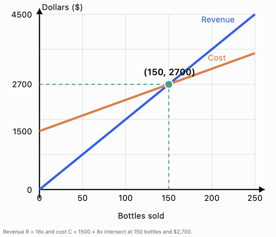
Interpreting the graph
Before the intersection:
Cost is greater than revenue.
The business operates at a loss.
At the intersection:
Revenue equals cost.
The business breaks even.
After the intersection:
Revenue is greater than cost.
The business earns a profit.
Important assumptions
This linear model assumes that:
-
The selling price remains constant.
-
Variable cost per unit remains constant.
-
Fixed costs remain unchanged.
-
All produced units are sold.
-
The business has sufficient production capacity.
Real businesses may experience changing prices, discounts, additional costs, and production limits.
Therefore, the model is useful but simplified.
Application: Comparing Two Business Plans
A company is considering two ways to manufacture a product.
Plan A
Fixed costs: $2,000
Variable cost: $5 per unit
Plan B
Fixed costs: $800
Variable cost: $9 per unit
The company wants to know which plan is cheaper at different production levels.
Step 1: Define the variable
x = number of units manufactured
Step 2: Construct the cost equations
Plan A:
Cₐ = 2000 + 5x
Plan B:
Cᵦ = 800 + 9x
Step 3: Find the intersection
At the intersection, both plans have the same cost.
2000 + 5x = 800 + 9x
1200 = 4x
x = 300
Step 4: Calculate the cost
Plan A:
Cₐ = 2000 + 5(300)
Cₐ = $3500
Plan B:
Cᵦ = 800 + 9(300)
Cᵦ = $3500
The two plans cost the same when 300 units are manufactured.
Step 5: Compare different production levels
|
Units produced |
Plan A |
Plan B |
Cheaper plan |
|---|---|---|---|
|
100 |
$2,500 |
$1,700 |
B |
|
200 |
$3,000 |
$2,600 |
B |
|
300 |
$3,500 |
$3,500 |
Equal |
|
400 |
$4,000 |
$4,400 |
A |
|
500 |
$4,500 |
$5,300 |
A |
Business conclusion
Plan B is cheaper for fewer than 300 units because it has lower fixed costs.
Plan A is cheaper for more than 300 units because it has a lower variable cost per unit.
The decision depends on expected production volume.
This example demonstrates how solving a system can identify the point at which one business strategy becomes more economical than another.
Application: Finding Fixed and Variable Costs
A manufacturer records the following production costs:
-
Producing 100 units costs $1,400.
-
Producing 250 units costs $2,600.
Assuming a linear cost model, determine the fixed cost and variable cost per unit.
Step 1: Define variables
F = fixed cost, in dollars
v = variable cost per unit, in dollars
The model is:
C = F + vx
Step 2: Construct equations
For 100 units:
F + 100v = 1400
For 250 units:
F + 250v = 2600
Step 3: Eliminate F
Subtract the first equation from the second:
150v = 1200
v = 8
Step 4: Find F
F + 100(8) = 1400
F + 800 = 1400
F = 600
Step 5: Interpret
Fixed cost = $600
Variable cost = $8 per unit
Therefore:
C = 600 + 8x
Step 6: Verify
At 100 units:
C = 600 + 8(100) = $1400
At 250 units:
C = 600 + 8(250) = $2600
Both values match the original data.
Business conclusion
The company spends $600 regardless of production volume within the model's operating range, plus $8 for each unit manufactured.
This information can help the business forecast costs at other production levels.
Application: Determining Product Prices from Sales
A school shop sells notebooks and pens.
On Monday, it sells 30 notebooks and 20 pens for $190.
On Tuesday, it sells 20 notebooks and 40 pens for $200.
Find the selling price of each item.
Step 1: Define variables
n = selling price of one notebook
p = selling price of one pen
Step 2: Construct equations
Monday:
30n + 20p = 190
Tuesday:
20n + 40p = 200
Step 3: Simplify
Divide the first equation by 10:
3n + 2p = 19
Divide the second equation by 20:
n + 2p = 10
Step 4: Eliminate p
Subtract the second equation from the first:
2n = 9
n = 4.50
Step 5: Find p
4.50 + 2p = 10
2p = 5.50
p = 2.75
Step 6: Verify
Monday:
30(4.50) + 20(2.75)
= 135 + 55 = $190
Tuesday:
20(4.50) + 40(2.75)
= 90 + 110 = $200
Answer: Notebooks sell for $4.50 and pens sell for $2.75.
Economic interpretation
The system determines the prices that are consistent with both days' sales records, assuming the prices were unchanged and the recorded revenue came only from these items.
Application: Three Products and Total Revenue
A company sells three products: A, B, and C.
Their selling prices are:
-
Product A: $10
-
Product B: $15
-
Product C: $20
During one day, the company sells 100 products and earns $1,500.
It sells 20 more units of Product A than Product C.
Find the quantity of each product sold.
Step 1: Define variables
a = number of Product A units
b = number of Product B units
c = number of Product C units
Step 2: Construct equations
Total units:
a + b + c = 100
Revenue:
10a + 15b + 20c = 1500
Relationship:
a − c = 20
Step 3: Eliminate a
Multiply the total quantity equation by 10:
10a + 10b + 10c = 1000
Subtract from the revenue equation:
5b + 10c = 500
Divide by 5:
b + 2c = 100
Step 4: Use the third equation
a = c + 20
Substitute into the total quantity equation:
c + 20 + b + c = 100
b + 2c = 80
Step 5: Interpret the contradiction
The system requires both:
b + 2c = 100
and:
b + 2c = 80
These cannot both be true.
Therefore, the sales records are inconsistent.
Answer: No solution exists for the stated information.
What could this mean for the business?
Possible explanations include incorrect sales totals, inaccurate revenue records, or an incorrect statement about the relationship between products A and C.
A system of equations can therefore help identify problems in business data, not just calculate unknown quantities.
A consistent version
Suppose the revenue was $1,400 rather than $1,500.
The revenue equation becomes:
10a + 15b + 20c = 1400
Subtracting 10 times the quantity equation gives:
b + 2c = 80
This is the same relationship obtained from a = c + 20.
The revised system has infinitely many solutions, not one unique solution.
An additional independent piece of information would be required to determine the exact quantities.
This illustrates an important limitation: three equations do not guarantee a unique solution if some equations contain redundant information.
Application: Production Planning with Three Products
A factory produces three types of furniture: chairs, tables, and shelves.
Each product requires a different amount of assembly time.
|
Product |
Assembly time per unit |
|---|---|
|
Chair |
2 hours |
|
Table |
4 hours |
|
Shelf |
3 hours |
The factory manufactures 100 items using 290 assembly-hours.
It manufactures 10 more chairs than shelves.
Determine the number of each product.
Step 1: Define variables
c = chairs manufactured
t = tables manufactured
s = shelves manufactured
Step 2: Construct equations
Total items:
c + t + s = 100
Total assembly time:
2c + 4t + 3s = 290
Quantity relationship:
c − s = 10
Step 3: Eliminate c
Multiply the first equation by 2:
2c + 2t + 2s = 200
Subtract from the assembly-time equation:
2t + s = 90
Step 4: Use the relationship
c = s + 10
Substitute into the total quantity equation:
s + 10 + t + s = 100
t + 2s = 90
Step 5: Solve the reduced system
We have:
2t + s = 90
t + 2s = 90
Multiply the second equation by 2:
2t + 4s = 180
Subtract the first equation:
3s = 90
s = 30
Then:
t + 2(30) = 90
t = 30
And:
c = 30 + 10 = 40
Step 6: Verify
Total items:
40 + 30 + 30 = 100
Assembly time:
2(40) + 4(30) + 3(30)
= 80 + 120 + 90
= 290 hours
Quantity relationship:
40 − 30 = 10
Answer: 40 chairs, 30 tables, and 30 shelves.
Business conclusion
The factory's production records are consistent with manufacturing 40 chairs, 30 tables, and 30 shelves.
This information could be used to estimate material requirements, labour costs, and future production capacity.
Application: Profit Targets
A business sells handmade bags for $35 each.
The variable cost is $15 per bag.
Monthly fixed costs are $2,400.
The owner wants to earn a monthly profit of $1,600.
How many bags must be sold?
Step 1: Define the variable
x = number of bags sold
Step 2: Write the revenue equation
R = 35x
Step 3: Write the cost equation
C = 2400 + 15x
Step 4: Write the profit equation
P = R − C
P = 35x − (2400 + 15x)
P = 20x − 2400
Step 5: Set the target profit
1600 = 20x − 2400
4000 = 20x
x = 200
Step 6: Verify
Revenue:
35(200) = $7000
Total cost:
2400 + 15(200) = $5400
Profit:
7000 − 5400 = $1600
Answer: The business must sell 200 bags to achieve the target profit of $1,600.
Understanding Contribution Margin
The contribution margin per unit is the selling price minus the variable cost per unit.
Contribution margin = p − v
For this business:
35 − 15 = $20 per bag
Each bag sold contributes $20 toward covering fixed costs and generating profit.
This allows us to write:
P = (p − v)x − F
For a target profit T:
x = (F + T)/(p − v)
provided p − v is positive.
In this example:
x = (2400 + 1600)/(35 − 15)
x = 4000/20
x = 200 bags
When the answer is not a whole number
Suppose the calculation gives:
x = 152.4
If x represents complete products, the business generally needs to sell at least 153 products to reach or exceed its target, assuming the contribution margin is positive.
Rounding down would not achieve the required profit.
Application: Comparing Profit Between Two Businesses
Two businesses sell the same type of product.
Business A has:
-
Selling price: $25 per unit
-
Variable cost: $10 per unit
-
Fixed cost: $1,500
Business B has:
-
Selling price: $25 per unit
-
Variable cost: $7 per unit
-
Fixed cost: $2,400
At what sales volume do the businesses earn the same profit?
Step 1: Construct the profit equations
Business A:
Pₐ = 25x − (1500 + 10x)
Pₐ = 15x − 1500
Business B:
Pᵦ = 25x − (2400 + 7x)
Pᵦ = 18x − 2400
Step 2: Set the profits equal
15x − 1500 = 18x − 2400
900 = 3x
x = 300
Step 3: Calculate the profit
Business A:
Pₐ = 15(300) − 1500 = $3000
Business B:
Pᵦ = 18(300) − 2400 = $3000
Both businesses earn $3,000 profit at 300 units sold.
Step 4: Interpret
Below 300 units, Business A earns more profit because it has lower fixed costs.
Above 300 units, Business B earns more profit because its variable cost per unit is lower.
Comparison table
|
Units sold |
Business A profit |
Business B profit |
|---|---|---|
|
100 |
$0 |
−$600 |
|
200 |
$1,500 |
$1,200 |
|
300 |
$3,000 |
$3,000 |
|
400 |
$4,500 |
$4,800 |
|
500 |
$6,000 |
$6,600 |
Business conclusion
The better business model depends on expected sales volume.
A business expecting relatively low sales may prefer lower fixed costs, while one expecting higher sales may benefit from lower variable costs.
Applications in Economics: Supply and Demand
Systems of equations are also used to model markets.
Two important economic concepts are supply and demand.
Demand
Demand describes how much of a product consumers are willing and able to purchase at different prices.
In a simple linear model, quantity demanded decreases as price increases.
For example:
Qd = 100 − 2p
where:
Qd = quantity demanded
p = price
Supply
Supply describes how much producers are willing and able to sell at different prices.
In a simple linear model, quantity supplied increases as price increases.
For example:
Qs = 20 + 2p
Market Equilibrium
Market equilibrium occurs when:
Qd = Qs
This is the price at which quantity demanded equals quantity supplied in the model.
Worked Example: Finding Equilibrium Price
Demand equation:
Qd = 100 − 2p
Supply equation:
Qs = 20 + 2p
At equilibrium:
100 − 2p = 20 + 2p
80 = 4p
p = 20
Substitute into demand:
Qd = 100 − 2(20)
Qd = 60
Substitute into supply:
Qs = 20 + 2(20)
Qs = 60
Equilibrium price = $20
Equilibrium quantity = 60 units
Interpreting the result
At a price of $20, consumers demand 60 units and producers supply 60 units.
At prices below equilibrium, the model predicts that quantity demanded exceeds quantity supplied.
At prices above equilibrium, the model predicts that quantity supplied exceeds quantity demanded.
Important limitation
Real markets are influenced by many factors, including consumer preferences, competition, income, taxes, and changes in production costs.
Linear supply-and-demand equations are simplified models, not exact predictions of every market.
Application: Comparing Subscription Plans
A business is choosing between two software subscriptions.
Plan A charges:
$50 per month plus $4 per user.
Plan B charges:
$110 per month plus $2 per user.
Find the number of users at which the plans cost the same.
Step 1: Define the variable
x = number of users
Step 2: Construct equations
Plan A:
Cₐ = 50 + 4x
Plan B:
Cᵦ = 110 + 2x
Step 3: Set costs equal
50 + 4x = 110 + 2x
2x = 60
x = 30
Step 4: Verify
Plan A:
50 + 4(30) = $170
Plan B:
110 + 2(30) = $170
Answer: Both plans cost $170 per month for 30 users.
Business interpretation
For fewer than 30 users, Plan A is cheaper.
For more than 30 users, Plan B is cheaper.
At exactly 30 users, both plans have the same monthly cost.
This type of comparison is useful when choosing subscriptions, equipment leases, service providers, or production arrangements.
Using Technology in Business Modelling
Spreadsheets and graphing software are useful for business analysis.
For example, a spreadsheet can calculate revenue, cost, and profit for many different sales volumes.
Consider:
R = 18x
C = 1500 + 8x
P = 10x − 1500
A spreadsheet could generate the following table.
|
Units sold |
Revenue |
Total cost |
Profit |
|---|---|---|---|
|
0 |
$0 |
$1,500 |
−$1,500 |
|
50 |
$900 |
$1,900 |
−$1,000 |
|
100 |
$1,800 |
$2,300 |
−$500 |
|
150 |
$2,700 |
$2,700 |
$0 |
|
200 |
$3,600 |
$3,100 |
$500 |
|
250 |
$4,500 |
$3,500 |
$1,000 |
The table makes the break-even point easy to identify.
Using graphing software
You can enter:
y = 18x
y = 1500 + 8x
into Desmos Graphing Calculator or GeoGebra Graphing Calculator.
The intersection represents the break-even point.
Technology is particularly useful when businesses need to compare several scenarios or change assumptions.
Evaluating the Reasonableness of Business Solutions
A mathematical answer must make sense in the business context.
Check 1: Units
If x represents the number of products sold, the answer should be expressed in units, not dollars.
If P represents profit, the answer should be expressed in money.
Check 2: Whole numbers
If a calculation gives:
x = 125.6 products
the business cannot normally sell 0.6 of a complete product.
If the goal is to meet or exceed a minimum profit, round up to 126 products when the model supports doing so.
Check 3: Negative values
A negative profit represents a loss.
However, a negative number of products sold is usually invalid in a simple sales model.
Check 4: Capacity
A company may calculate that it needs to sell 5,000 units to achieve its target.
But if it can only produce 3,000 units, the target cannot be reached under the current model.
Check 5: Model assumptions
A linear model assumes constant rates.
Real businesses may experience:
-
Bulk discounts.
-
Changes in labour costs.
-
Limited production capacity.
-
Seasonal demand.
-
Changing selling prices.
-
Additional fixed costs at higher output levels.
These factors can make a simple linear model less accurate.
Check 6: Verification
Always substitute calculated values into the original equations.
For example, if a system predicts that 40 units of A and 30 units of B generate $1,100:
20(40) + 10(30) = 1100
800 + 300 = 1100
The revenue equation is satisfied.
But other conditions must also be checked.
Communicating Mathematical Conclusions
In business and economics, a numerical answer is often not enough.
A complete conclusion should explain what the result means and how it can support a decision.
Example: Weak conclusion
x = 300
Improved conclusion
The two production plans have equal costs when 300 units are manufactured.
Strong conclusion
The two production plans each cost $3,500 at a production level of 300 units. Plan B is cheaper below 300 units because it has lower fixed costs, while Plan A is cheaper above 300 units because it has lower variable costs. Therefore, the company should consider its expected production volume before choosing a plan.
The final conclusion connects the mathematical result to a practical business decision.
A useful structure
When communicating a business solution, include:
-
Result: State the numerical answer with units.
-
Meaning: Explain what the value represents.
-
Verification: Show that it satisfies the original conditions.
-
Recommendation: Explain what the result suggests.
-
Limitation: Identify any assumptions that could affect the decision.
Common Mistakes
Confusing revenue with profit
Revenue is money received from sales. Profit is revenue minus total costs.
Forgetting fixed costs
A business may lose money even when each product sells for more than its variable production cost.
Using the wrong break-even equation
Break-even occurs when total revenue equals total cost, not when revenue equals variable cost alone.
Mixing prices and quantities
The selling price of a product and the number of products sold are different variables.
Constructing incorrect revenue equations
Revenue is calculated by multiplying price by quantity.
Forgetting to include all products
When several products are sold, total revenue must include the revenue from every product.
Rounding sales quantities incorrectly
When calculating the minimum number of complete units required to reach a profit target, round up when appropriate.
Assuming every system has a unique solution
Some business systems contain redundant or contradictory information.
Ignoring production capacity
A mathematically possible sales target may be impossible with existing resources.
Accepting unrealistic negative quantities
Negative profit may be meaningful, but negative quantities of physical products are generally not.
Failing to explain the result
Business conclusions should describe the meaning of the answer, not just provide a number.
Ignoring assumptions
Constant selling prices and costs may not remain realistic over large production ranges.
Key Terms
-
Fixed cost: A cost that remains constant over the relevant production range.
-
Variable cost: A cost that changes with production volume.
-
Total cost: The combined fixed and variable costs.
-
Revenue: Money received from sales.
-
Profit: Revenue minus total cost.
-
Loss: A negative profit.
-
Break-even point: The sales volume at which revenue equals total cost.
-
Contribution margin: Selling price minus variable cost per unit.
-
Selling price: The amount charged for a product or service.
-
Unit cost: The cost associated with one unit.
-
Production volume: The number of units manufactured.
-
Sales volume: The number of units sold.
-
Profit target: A desired amount of profit.
-
Cost model: An equation representing how costs depend on production or activity.
-
Revenue model: An equation representing income from sales.
-
Supply: The quantity producers are willing and able to sell at different prices.
-
Demand: The quantity consumers are willing and able to buy at different prices.
-
Market equilibrium: The point where quantity supplied equals quantity demanded.
-
Constraint: A restriction on possible values or decisions.
-
Mathematical model: A representation of a real-world situation using equations.
-
Verification: Checking that a solution satisfies the original equations.
-
Reasonableness: Evaluating whether a mathematical result makes sense in context.
Key Takeaways
-
Systems of equations can model costs, revenue, profit, and production.
-
Total cost can be represented by C = F + vx.
-
Revenue can be represented by R = px when selling price is constant.
-
Profit is calculated using P = R − C.
-
Break-even occurs when revenue equals total cost.
-
Systems can compare two business plans and identify when their costs or profits are equal.
-
Two or more sales records can help determine unknown prices or quantities.
-
Three-variable systems can model production involving several products.
-
Supply-and-demand systems can determine market equilibrium in simplified economic models.
-
Mathematical solutions should be interpreted using appropriate units.
-
Business decisions should consider capacity, realistic quantities, and model assumptions.
-
Strong conclusions explain what a solution means and how it supports a decision.
Check Your Understanding
Recall and Understanding
1. Explain the difference between fixed costs and variable costs. Give one example of each.
2. Define revenue, cost, and profit.
3. What does the break-even point represent?
4. Explain why a business might prefer a production method with higher fixed costs but lower variable costs.
5. Why should a business evaluate the assumptions of a mathematical model before using it to make decisions?
Cost and Profit Problems
6. A company sells water bottles for $20 each. Variable costs are $8 per bottle, and fixed costs are $1,200.
a. Write the revenue equation.
b. Write the total cost equation.
c. Write the profit equation.
d. Find the break-even quantity.
7. A business sells products for $30 each. Variable costs are $12 per unit, and fixed costs are $1,800.
How many products must be sold to earn a profit of $1,800?
8. A manufacturer has fixed costs of $750 and variable costs of $6 per unit.
Calculate the total cost of producing 200 units.
9. A company records total costs of $1,500 when producing 100 units and $2,700 when producing 300 units.
Assuming a linear cost model, determine the fixed cost and variable cost per unit.
10. A company sells 250 products at $24 each. Total costs are $4,200.
Calculate revenue and profit.
Systems and Business Applications
11. Two companies offer production services.
Plan A: $1,000 fixed cost plus $8 per unit.
Plan B: $400 fixed cost plus $12 per unit.
Find the production quantity at which the plans cost the same.
12. A school sells adult tickets for $15 and student tickets for $10.
A total of 120 tickets are sold, generating $1,500.
Determine the number of each ticket type.
13. A shop sells notebooks and pens.
Three notebooks and two pens cost $23.
Two notebooks and four pens cost $26.
Find the price of each item.
14. A factory manufactures chairs, tables, and shelves.
It produces 100 items using 290 assembly-hours.
Each chair requires 2 hours, each table 4 hours, and each shelf 3 hours.
The factory produces 10 more chairs than shelves.
Determine the number of each product.
15. The demand and supply equations for a product are:
Qd = 120 − 3p
Qs = 20 + 2p
Find the equilibrium price and quantity.
Challenge
16. A company sells a product for $25 per unit. Its fixed costs are $2,000, and its variable costs are $10 per unit.
The company can produce at most 180 units.
Can it achieve a profit of $1,000? Explain using calculations.
17. A business compares two profit models:
Pₐ = 12x − 900
Pᵦ = 15x − 1500
Determine when the profits are equal and which model is better for higher sales volumes.
18. A company sells two products.
Product A sells for $20 and Product B for $30.
The company sells 100 units and earns $2,400.
Find the quantity of each product.
19. A manufacturer calculates that it must sell 175.4 units to reach a profit target.
Explain how the answer should be interpreted if only complete units can be sold.
20. A business reports:
x + y + z = 100
2x + 3y + 4z = 290
x − z = 10
Solve the system and explain what the solution could represent in a production context.
Answers to Check Your Understanding
1. Fixed and variable costs
Fixed costs remain unchanged over the relevant production range, such as monthly rent.
Variable costs change with the number of units produced, such as raw materials or packaging.
2. Revenue, cost, and profit
Revenue is money received from sales.
Cost is money spent to operate the business or produce goods.
Profit is the difference:
P = R − C
3. Break-even point
The break-even point is where total revenue equals total cost.
At this point, profit is zero.
4. Higher fixed costs and lower variable costs
A company with higher fixed costs but lower variable costs may become cheaper at high production volumes.
The lower variable cost can eventually offset the higher fixed cost.
5. Evaluating assumptions
Mathematical models simplify real situations.
For example, a linear model may assume constant selling prices, fixed costs, and variable costs.
If these assumptions do not hold, the model's predictions may become inaccurate.
6. Water bottle business
Given:
Selling price = $20
Variable cost = $8
Fixed cost = $1,200
a. Revenue:
R = 20x
b. Total cost:
C = 1200 + 8x
c. Profit:
P = 20x − (1200 + 8x)
P = 12x − 1200
d. Break-even:
20x = 1200 + 8x
12x = 1200
x = 100
Answer: The business breaks even at 100 bottles.
Verification:
Revenue = 20(100) = $2000
Cost = 1200 + 8(100) = $2000
7. Profit target
Selling price = $30
Variable cost = $12
Fixed cost = $1800
Target profit = $1800
Profit equation:
P = 30x − (1800 + 12x)
P = 18x − 1800
Set the target:
1800 = 18x − 1800
3600 = 18x
x = 200
Answer: 200 products.
Verification:
Revenue = 30(200) = $6000
Cost = 1800 + 12(200) = $4200
Profit = $1800
8. Total production cost
C = F + vx
C = 750 + 6(200)
C = 750 + 1200
Answer: $1,950.
9. Finding fixed and variable costs
Let:
F = fixed cost
v = variable cost per unit
Construct equations:
F + 100v = 1500
F + 300v = 2700
Subtract:
200v = 1200
v = 6
Substitute:
F + 100(6) = 1500
F = 900
Answer: Fixed cost = $900; variable cost = $6 per unit.
Cost equation:
C = 900 + 6x
10. Revenue and profit
Revenue:
R = 250(24)
R = $6000
Profit:
P = R − C
P = 6000 − 4200
Answer: Revenue = $6,000; profit = $1,800.
11. Comparing production plans
Plan A:
Cₐ = 1000 + 8x
Plan B:
Cᵦ = 400 + 12x
Set costs equal:
1000 + 8x = 400 + 12x
600 = 4x
x = 150
Calculate cost:
1000 + 8(150) = $2200
400 + 12(150) = $2200
Answer: Both plans cost $2,200 at 150 units.
Below 150 units, Plan B is cheaper.
Above 150 units, Plan A is cheaper.
12. Ticket sales
Let:
a = adult tickets
s = student tickets
Equations:
a + s = 120
15a + 10s = 1500
Multiply the first equation by 10:
10a + 10s = 1200
Subtract:
5a = 300
a = 60
Then:
s = 120 − 60
s = 60
Answer: 60 adult tickets and 60 student tickets.
Verification:
60 + 60 = 120
15(60) + 10(60) = $1500
13. Notebook and pen prices
Let:
n = notebook price
p = pen price
Equations:
3n + 2p = 23
2n + 4p = 26
Multiply the first equation by 2:
6n + 4p = 46
Subtract the second equation:
4n = 20
n = 5
Substitute:
3(5) + 2p = 23
2p = 8
p = 4
Answer: Notebook = $5; pen = $4.
Verification:
3(5) + 2(4) = 23
2(5) + 4(4) = 26
14. Furniture production
Let:
c = chairs
t = tables
s = shelves
Equations:
c + t + s = 100
2c + 4t + 3s = 290
c − s = 10
From the third equation:
c = s + 10
Substitute into the total quantity equation:
t + 2s = 90
Substitute into the assembly-time equation:
2(s + 10) + 4t + 3s = 290
4t + 5s = 270
Multiply t + 2s = 90 by 4:
4t + 8s = 360
Subtract:
3s = 90
s = 30
Then:
t = 90 − 2(30) = 30
c = 30 + 10 = 40
Answer: 40 chairs, 30 tables, and 30 shelves.
Verification:
40 + 30 + 30 = 100
2(40) + 4(30) + 3(30) = 290
15. Market equilibrium
Demand:
Qd = 120 − 3p
Supply:
Qs = 20 + 2p
At equilibrium:
120 − 3p = 20 + 2p
100 = 5p
p = 20
Substitute:
Q = 120 − 3(20)
Q = 60
Answer: Equilibrium price = $20; equilibrium quantity = 60 units.
Verification:
Demand = 60
Supply = 20 + 2(20) = 60
16. Profit target and capacity
Selling price = $25
Variable cost = $10
Fixed cost = $2000
Maximum production = 180 units
Profit equation:
P = 25x − (2000 + 10x)
P = 15x − 2000
To earn $1000:
1000 = 15x − 2000
3000 = 15x
x = 200
However, the company can only produce 180 units.
Maximum profit at full capacity:
P = 15(180) − 2000
P = 2700 − 2000
P = $700
Answer: No. The company cannot achieve a $1,000 profit under the stated conditions. Its maximum possible profit is $700 if it produces and sells all 180 units.
17. Comparing profit models
Pₐ = 12x − 900
Pᵦ = 15x − 1500
Set equal:
12x − 900 = 15x − 1500
600 = 3x
x = 200
Calculate profit:
Pₐ = 12(200) − 900 = $1500
Pᵦ = 15(200) − 1500 = $1500
Answer: Both models produce $1,500 profit at 200 units.
For more than 200 units, Model B produces greater profit because its profit increases by $15 per additional unit compared with $12 for Model A.
18. Two-product sales
Let:
a = units of Product A
b = units of Product B
Total quantity:
a + b = 100
Revenue:
20a + 30b = 2400
Multiply the first equation by 20:
20a + 20b = 2000
Subtract:
10b = 400
b = 40
Then:
a = 60
Answer: 60 units of Product A and 40 units of Product B.
Verification:
60 + 40 = 100
20(60) + 30(40) = $2400
19. Fractional sales quantity
The calculated quantity is:
x = 175.4
If the business must sell complete units and needs to reach or exceed a profit target, it should round up.
Answer: The business must sell at least 176 units, assuming profit increases with each additional unit and the model remains valid.
Rounding down to 175 would leave the business below its target.
20. Three-product production
Given:
x + y + z = 100
2x + 3y + 4z = 290
x − z = 10
From the third equation:
x = z + 10
Substitute into the first:
(z + 10) + y + z = 100
y + 2z = 90
Substitute into the second:
2(z + 10) + 3y + 4z = 290
3y + 6z = 270
Divide by 3:
y + 2z = 90
Both reduced equations are identical.
Therefore, the system does not have a unique solution.
Let z = t.
Then:
x = t + 10
y = 90 − 2t
The general solution is:
(x, y, z) = (t + 10, 90 − 2t, t)
For nonnegative quantities:
0 ≤ t ≤ 45
If the variables represent complete products, t must be an integer.
For example, one possible production combination is:
x = 40
y = 30
z = 30
Verification:
40 + 30 + 30 = 100
2(40) + 3(30) + 4(30) = 290
40 − 30 = 10
Answer: The system has infinitely many nonnegative real solutions and 46 possible whole-number production combinations.
An additional independent condition would be needed to determine the exact production quantities.
Final Summary
Systems of equations provide a practical foundation for analysing business and economic situations.
They can be used to calculate costs, determine prices, establish profit targets, identify break-even points, compare business strategies, and investigate supply-and-demand relationships.
However, mathematical calculations are only part of effective business decision-making. Results must be verified, interpreted using appropriate units, and evaluated against real-world constraints.
The most valuable business solution is not simply a correct number, but a well-supported conclusion that helps explain a situation and guide a decision.
2. Science Applications
Learning outcomes
- I can apply systems of equations in scientific contexts.
- I can model experimental situations.
- I can solve scientific problems using systems.
- I can interpret results with appropriate units.
- I can evaluate the limitations of mathematical models.
Introduction
Science uses mathematics to describe, explain, and predict how the natural world behaves. Whether scientists are studying the motion of objects, analysing chemical reactions, measuring electrical circuits, or investigating experimental data, they frequently encounter situations involving several unknown quantities.
A system of equations allows scientists to combine different pieces of information and determine unknown values.
For example, a scientist might need to determine:
-
The masses of two substances in a mixture.
-
The speeds of two moving objects.
-
The forces acting on an object in equilibrium.
-
The currents flowing through different parts of an electrical circuit.
-
The concentrations of solutions prepared in a laboratory.
-
The unknown parameters in an experimental model.
Each measurement or scientific law provides a mathematical relationship. When enough independent relationships are available, the unknown quantities can often be determined.
Systems of equations are especially useful because they allow scientists to analyse several connected quantities simultaneously.
However, scientific models are simplified representations of reality. A mathematically correct solution must still be evaluated using scientific principles, appropriate units, experimental uncertainty, and the assumptions of the model.
Why Are Systems of Equations Important in Science?
Scientific investigations often involve multiple unknown quantities.
Consider a laboratory mixture containing two liquids.
A scientist knows:
-
The total volume of the mixture.
-
The total mass of the mixture.
-
The densities of the two liquids.
The scientist wants to determine the volume of each liquid.
One equation can describe the total volume.
Another equation can describe the total mass.
Together, these equations form a system that can determine both unknown volumes.
This approach is used across many scientific disciplines.
|
Scientific field |
Example application |
Possible unknowns |
|---|---|---|
|
Physics |
Motion of two objects |
Speeds, times, distances |
|
Chemistry |
Preparing solutions |
Volumes, concentrations |
|
Biology |
Population studies |
Numbers of different organisms |
|
Electricity |
Analysing circuits |
Currents, voltages |
|
Mechanics |
Force equilibrium |
Tensions, reaction forces |
|
Environmental science |
Pollutant mixing |
Masses, concentrations |
|
Experimental science |
Analysing data |
Gradient, intercept, model parameters |
The general process is similar in every field:
Scientific information → Mathematical equations → Solution → Scientific interpretation → Verification
Building a Mathematical Model from Scientific Information
A mathematical model represents a scientific situation using variables and equations.
A reliable modelling process involves several steps.
Step 1: Identify the unknown quantities
Define variables clearly and include their units.
For example:
m₁ = mass of substance A, in grams
m₂ = mass of substance B, in grams
Step 2: Identify the scientific relationships
Look for relevant scientific laws or definitions.
Examples include:
Speed = distance/time
Density = mass/volume
Force = mass × acceleration
Charge = current × time
Concentration = mass of solute/volume of solution
Step 3: Construct equations
Use the information in the problem to create relationships between the variables.
Step 4: Solve the system
Choose an appropriate method:
-
Substitution.
-
Elimination.
-
Graphing.
-
Matrix methods.
-
Technology.
Step 5: Interpret the solution
Explain what each value represents and include correct units.
Step 6: Verify the result
Substitute the values into the original equations and check whether they satisfy the scientific conditions.
Step 7: Evaluate the model
Consider whether the assumptions are realistic and whether the measurements are sufficiently accurate.
Application: Mixing Two Liquids Using Density
Density describes how much mass is contained in a given volume.
The density equation is:
ρ = m/V
where:
-
ρ = density.
-
m = mass.
-
V = volume.
Rearranging:
m = ρV
Suppose a laboratory technician mixes two liquids.
Liquid A has a density of 0.8 g/mL.
Liquid B has a density of 1.2 g/mL.
The mixture has:
-
Total volume = 100 mL.
-
Total mass = 104 g.
Assuming the volumes are additive, determine the volume of each liquid.
Step 1: Define variables
x = volume of Liquid A, in mL
y = volume of Liquid B, in mL
Step 2: Construct the volume equation
The total volume is 100 mL.
x + y = 100
Step 3: Construct the mass equation
Mass = density × volume
Liquid A has mass:
0.8x
Liquid B has mass:
1.2y
The total mass is 104 g.
0.8x + 1.2y = 104
Step 4: Solve by substitution
From the volume equation:
x = 100 − y
Substitute:
0.8(100 − y) + 1.2y = 104
80 − 0.8y + 1.2y = 104
0.4y = 24
y = 60
Then:
x = 100 − 60
x = 40
Step 5: Interpret
Liquid A: 40 mL
Liquid B: 60 mL
Step 6: Verify
Total volume:
40 + 60 = 100 mL
Total mass:
0.8(40) + 1.2(60)
= 32 + 72
= 104 g
Both conditions are satisfied.
Answer: The mixture contains 40 mL of Liquid A and 60 mL of Liquid B.
Limitations of the model
The calculation assumes that the volumes are additive.
In real mixtures, molecular interactions can cause the final volume to differ from the sum of the separate volumes.
The model also assumes that the densities remain constant at the experimental temperature.
These assumptions must be considered before applying the result to an actual laboratory mixture.
Application: Preparing Solutions of Different Concentrations
Scientists often prepare solutions by combining liquids with different concentrations.
Suppose a laboratory needs 500 mL of a 20% solution.
Two solutions are available:
-
Solution A: 10%.
-
Solution B: 30%.
How much of each solution is required?
Step 1: Define variables
x = volume of 10% solution, in mL
y = volume of 30% solution, in mL
Step 2: Total volume equation
x + y = 500
Step 3: Solute equation
The amount of solute in each solution is proportional to its concentration.
0.10x + 0.30y = 0.20(500)
Therefore:
0.10x + 0.30y = 100
The equation uses equivalent volumes of solute under a simplified volume-percent model.
Step 4: Solve
From the first equation:
x = 500 − y
Substitute:
0.10(500 − y) + 0.30y = 100
50 − 0.10y + 0.30y = 100
0.20y = 50
y = 250
Then:
x = 500 − 250
x = 250
Step 5: Interpret
250 mL of the 10% solution
250 mL of the 30% solution
Step 6: Verify
Total volume:
250 + 250 = 500 mL
Solute-equivalent volume:
0.10(250) + 0.30(250)
= 25 + 75
= 100 mL
Final concentration:
100/500 × 100% = 20%
Answer: Mix 250 mL of each solution.
Scientific interpretation
The required concentration lies halfway between 10% and 30%.
Therefore, equal volumes produce the desired 20% concentration under the model's assumptions.
Important limitation
This simplified model assumes consistent concentration definitions and additive volumes. In laboratory work, concentration units such as mol/L, g/L, and mass percent must not be mixed without conversion.
For precise solution preparation, a laboratory may need to measure solute quantity and dilute to a specified final volume rather than simply add two measured volumes.
Application: Motion of Two Objects
Systems of equations can be used to analyse objects moving at constant speeds.
The basic relationship is:
d = vt
where:
-
d = distance.
-
v = speed.
-
t = time.
Worked Example: Two Cyclists
Two cyclists begin travelling from the same location in opposite directions.
After 3 hours, they are 90 km apart.
One cyclist travels 6 km/h faster than the other.
Find their speeds.
Step 1: Define variables
x = speed of the slower cyclist, in km/h
y = speed of the faster cyclist, in km/h
Step 2: Construct the distance equation
The slower cyclist travels:
3x kilometres
The faster cyclist travels:
3y kilometres
Since they travel in opposite directions, their separation is the sum of the distances.
3x + 3y = 90
Divide by 3:
x + y = 30
Step 3: Construct the speed equation
The faster cyclist travels 6 km/h faster.
y − x = 6
Step 4: Solve
Add the equations:
x + y = 30
−x + y = 6
2y = 36
y = 18
Then:
x = 30 − 18
x = 12
Step 5: Verify
Slower cyclist:
d = 12(3) = 36 km
Faster cyclist:
d = 18(3) = 54 km
Total separation:
36 + 54 = 90 km
Speed difference:
18 − 12 = 6 km/h
Answer: The slower cyclist travels at 12 km/h, and the faster cyclist travels at 18 km/h.
Limitations of the model
The calculation assumes that both cyclists:
-
Travel in exactly opposite directions along the same straight route.
-
Maintain constant speeds.
-
Start at the same time.
-
Do not stop during the journey.
Real journeys may involve acceleration, changes in direction, and stops.
The model is therefore an approximation of actual motion.
Application: Forces in Equilibrium
An object is in equilibrium when the resultant force acting on it is zero.
For equilibrium in two dimensions:
ΣFₓ = 0
ΣFᵧ = 0
These equations can be used together to determine unknown forces.
Worked Example: A Hanging Sign
A sign weighing 100 N is supported by two cables.
The left cable makes an angle of 30° above the horizontal.
The right cable makes an angle of 60° above the horizontal.
Determine the tension in each cable.
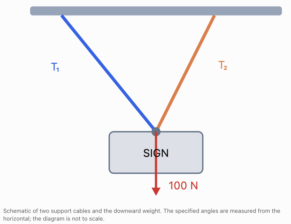
Step 1: Define variables
T₁ = tension in the left cable, in N
T₂ = tension in the right cable, in N
Step 2: Resolve the forces horizontally
The horizontal components must balance.
The left cable pulls left.
The right cable pulls right.
T₁ cos 30° = T₂ cos 60°
Using:
cos 30° ≈ 0.866
cos 60° = 0.5
We obtain:
0.866T₁ = 0.5T₂
Therefore:
T₂ ≈ 1.732T₁
Step 3: Resolve the forces vertically
The upward components must balance the 100 N weight.
T₁ sin 30° + T₂ sin 60° = 100
Using:
sin 30° = 0.5
sin 60° ≈ 0.866
We obtain:
0.5T₁ + 0.866T₂ = 100
Step 4: Substitute
0.5T₁ + 0.866(1.732T₁) ≈ 100
0.5T₁ + 1.5T₁ ≈ 100
2T₁ ≈ 100
T₁ ≈ 50 N
Then:
T₂ ≈ 1.732(50)
T₂ ≈ 86.6 N
Step 5: Interpret
Left cable tension ≈ 50 N
Right cable tension ≈ 86.6 N
The right cable has greater tension because its steeper angle changes how the force is distributed between horizontal and vertical components.
Step 6: Verify
Horizontal:
50 cos 30° ≈ 86.6 cos 60°
43.3 N ≈ 43.3 N
Vertical:
50 sin 30° + 86.6 sin 60°
≈ 25 + 75
≈ 100 N
Answer: T₁ = 50 N and T₂ ≈ 86.6 N.
Scientific assumptions
This model assumes:
-
The sign is stationary.
-
The cables are massless.
-
The cable angles are known accurately.
-
No additional horizontal forces act.
-
The sign is treated as a particle at the support junction, or the support geometry also satisfies rotational equilibrium.
In real engineering problems, the sign's dimensions, attachment points, and torque balance may also need to be considered.
Application: Electrical Circuits
Electrical circuits can be analysed using systems of equations.
Two important principles are:
Kirchhoff's Current Law
The total current entering a junction equals the total current leaving the junction.
Kirchhoff's Voltage Law
The sum of voltage changes around a closed circuit loop equals zero.
Ohm's Law is also important:
V = IR
where:
-
V = potential difference, in volts.
-
I = current, in amperes.
-
R = resistance, in ohms.
Worked Example: Currents in a Circuit
At a junction, a total current of 6 A splits into two branches.
The first branch has resistance 4 Ω.
The second branch has resistance 8 Ω.
Both branches are connected in parallel, so the potential difference across each branch is equal.
Find the current in each branch.
Step 1: Define variables
I₁ = current through the 4 Ω branch, in A
I₂ = current through the 8 Ω branch, in A
Step 2: Apply the current law
I₁ + I₂ = 6
Step 3: Apply Ohm's Law
The voltage across each branch is the same.
4I₁ = 8I₂
Divide by 4:
I₁ = 2I₂
Step 4: Solve
Substitute:
2I₂ + I₂ = 6
3I₂ = 6
I₂ = 2 A
Then:
I₁ = 4 A
Step 5: Verify
Total current:
4 + 2 = 6 A
Voltage across first branch:
V₁ = 4(4) = 16 V
Voltage across second branch:
V₂ = 8(2) = 16 V
Both branches have the same potential difference.
Answer: The 4 Ω branch carries 4 A, and the 8 Ω branch carries 2 A.
Scientific interpretation
The branch with lower resistance carries more current when the voltage is the same.
This agrees with Ohm's Law.
Model limitations
The calculation assumes ideal resistors with constant resistance.
In real circuits, resistance can change with temperature, and components may not behave ideally.
Application: Determining Unknown Quantities from Experimental Data
Scientific experiments often produce measurements that can be used to construct equations.
Consider a spring that follows Hooke's Law:
F = kx
where:
-
F = applied force, in newtons.
-
k = spring constant, in N/m.
-
x = extension, in metres.
A real experimental setup may also contain a constant force offset caused by calibration error or another systematic effect.
A more general linear model is:
F = kx + b
where b represents the force offset.
Worked Example: Finding the Spring Constant
An experiment produces the following data:
|
Extension, x (m) |
Measured force, F (N) |
|---|---|
|
0.02 |
3 |
|
0.06 |
7 |
Assume the relationship is linear.
Find k and b.
Step 1: Define variables
k = spring constant, in N/m
b = force offset, in N
Step 2: Construct equations
First measurement:
3 = 0.02k + b
Second measurement:
7 = 0.06k + b
Step 3: Eliminate b
Subtract:
7 − 3 = (0.06 − 0.02)k
4 = 0.04k
k = 100 N/m
Step 4: Find b
3 = 0.02(100) + b
3 = 2 + b
b = 1 N
Step 5: Write the model
F = 100x + 1
where F is in N and x is in m.
Step 6: Interpret
The gradient is 100 N/m.
This represents the spring constant in the linear model.
The intercept is 1 N.
This indicates that the measured force includes a constant offset.
Step 7: Verify
At x = 0.02 m:
F = 100(0.02) + 1 = 3 N
At x = 0.06 m:
F = 100(0.06) + 1 = 7 N
Both measurements are reproduced.
Limitations
Two data points always determine a straight line when their x-values are different.
However, this does not prove that the physical relationship is perfectly linear.
Scientists should collect additional measurements and examine whether the model remains appropriate.
The spring may also stop following Hooke's Law beyond its elastic limit.
Application: Determining a Linear Motion Model
A moving object has position described by:
s = vt + s₀
where:
-
s = position, in metres.
-
v = constant velocity, in m/s.
-
t = time, in seconds.
-
s₀ = initial position, in metres.
A motion sensor records:
At t = 2 s, s = 11 m.
At t = 5 s, s = 23 m.
Determine the velocity and initial position.
Step 1: Construct equations
11 = 2v + s₀
23 = 5v + s₀
Step 2: Eliminate s₀
Subtract:
12 = 3v
v = 4 m/s
Step 3: Find initial position
11 = 2(4) + s₀
s₀ = 3 m
Step 4: Write the motion model
s = 4t + 3
Step 5: Verify
At t = 2 s:
s = 4(2) + 3 = 11 m
At t = 5 s:
s = 4(5) + 3 = 23 m
Answer: Velocity = 4 m/s; initial position = 3 m.
Scientific interpretation
The object moves in the positive direction at a constant velocity of 4 m/s.
At t = 0, its position is 3 m.
Limitation
The model assumes constant velocity.
If the object accelerates, a linear position-time equation may no longer be appropriate.
Application: Biology and Population Studies
Systems of equations can be used to estimate populations when several measurements are available.
Worked Example: Two Species in a Habitat
An ecological survey identifies two species of animals in a protected habitat.
Species A has 4 legs per animal.
Species B has 2 legs per animal.
The survey records:
-
50 animals in total.
-
160 legs in total.
Determine the number of animals of each species.
Step 1: Define variables
x = number of four-legged animals
y = number of two-legged animals
Step 2: Construct equations
Total animals:
x + y = 50
Total legs:
4x + 2y = 160
Step 3: Solve
Multiply the first equation by 2:
2x + 2y = 100
Subtract from the second:
2x = 60
x = 30
Then:
y = 50 − 30
y = 20
Step 4: Verify
Total animals:
30 + 20 = 50
Total legs:
4(30) + 2(20)
= 120 + 40
= 160
Answer: There are 30 four-legged animals and 20 two-legged animals.
Scientific limitations
The model assumes:
-
Only the two specified species are present.
-
Every animal has the expected number of legs.
-
All animals are counted correctly.
-
The recorded observations are accurate.
In a real ecological investigation, incomplete observations and sampling errors may affect the results.
Application: Chemical Reactions and Conservation of Mass
Chemical reactions obey the law of conservation of mass.
In a closed system, the total mass of reactants equals the total mass of products.
Systems of equations can be used to determine unknown masses.
Worked Example: Formation of a Compound
Two elements, A and B, react to form a compound.
The total mass of the compound is 60 g.
The mass of element A is twice the mass of element B.
Find the mass of each element.
Step 1: Define variables
x = mass of element A, in g
y = mass of element B, in g
Step 2: Construct equations
Conservation of mass:
x + y = 60
Mass relationship:
x = 2y
Step 3: Solve
Substitute:
2y + y = 60
3y = 60
y = 20
Then:
x = 40
Step 4: Verify
40 + 20 = 60 g
40 = 2(20)
Answer: Element A contributes 40 g and element B contributes 20 g.
Scientific interpretation
The compound contains 40 g of element A and 20 g of element B.
The mass ratio is:
A : B = 2 : 1
This example assumes complete reaction, no loss of material, and that the compound contains only the two elements.
In actual chemistry, chemical formulae and mole ratios must also be considered when determining how elements combine.
Application: Three-Variable Scientific Systems
More complex scientific situations may involve three unknown quantities.
Worked Example: Three Materials in a Mixture
A laboratory combines three materials, A, B, and C.
Their densities are:
|
Material |
Density |
|---|---|
|
A |
1 g/mL |
|
B |
2 g/mL |
|
C |
3 g/mL |
The total volume is 100 mL.
The total mass is 210 g.
The volume of Material C is 10 mL greater than the volume of Material A.
Determine the volume of each material.
Step 1: Define variables
x = volume of Material A, in mL
y = volume of Material B, in mL
z = volume of Material C, in mL
Step 2: Construct equations
Total volume:
x + y + z = 100
Total mass:
x + 2y + 3z = 210
Volume relationship:
z − x = 10
Step 3: Eliminate x
Subtract the total volume equation from the mass equation:
y + 2z = 110
Step 4: Use the third equation
z = x + 10
Therefore:
x = z − 10
Substitute into the volume equation:
(z − 10) + y + z = 100
y + 2z = 110
The reduced equations are identical.
Step 5: Interpret
The system does not have a unique solution.
The third relationship is already implied by the total mass and volume equations.
We can express the solutions using z = t:
x = t − 10
y = 110 − 2t
z = t
For nonnegative volumes:
10 ≤ t ≤ 55
There are infinitely many nonnegative real solutions.
Scientific conclusion
The available measurements are insufficient to determine the exact volume of each material.
An additional independent measurement is required.
For example, measuring the volume of one component would allow the remaining volumes to be determined.
Why this example matters
Scientific investigations do not always provide enough information to determine every unknown.
Recognising insufficient information is an important part of scientific reasoning.
Improving Experimental Models with Additional Measurements
Suppose the scientist measures the volume of Material B and finds:
y = 30 mL
Using:
y + 2z = 110
30 + 2z = 110
2z = 80
z = 40 mL
Then:
x = z − 10
x = 30 mL
The volumes are:
Material A: 30 mL
Material B: 30 mL
Material C: 40 mL
Verify
Total volume:
30 + 30 + 40 = 100 mL
Total mass:
1(30) + 2(30) + 3(40)
= 30 + 60 + 120
= 210 g
Volume difference:
40 − 30 = 10 mL
Answer: 30 mL of A, 30 mL of B, and 40 mL of C.
The additional independent measurement allows a unique solution to be determined.
Using Experimental Data to Construct Systems
Scientists frequently collect measurements and use them to determine unknown parameters.
Consider a relationship of the form:
y = mx + b
where:
m = gradient
b = y-intercept
Suppose an experiment produces:
|
x |
y |
|---|---|
|
2 |
7 |
|
5 |
16 |
The equations are:
7 = 2m + b
16 = 5m + b
Subtract:
9 = 3m
m = 3
Then:
7 = 2(3) + b
b = 1
The model is:
y = 3x + 1
Interpreting the parameters
The gradient represents the rate of change of y with respect to x.
The intercept represents the predicted value of y when x = 0.
The scientific meaning and units of these parameters depend on what x and y represent.
For example, if y is distance in metres and x is time in seconds:
m = 3 m/s
b = 1 m
The equation becomes:
s = 3t + 1
Why More Experimental Data Is Often Better
Two measurements can determine the gradient and intercept of a straight line.
However, real experimental measurements contain uncertainty.
For example:
|
Time (s) |
Position (m) |
|---|---|
|
0 |
1.1 |
|
1 |
4.0 |
|
2 |
7.2 |
|
3 |
9.9 |
|
4 |
13.1 |
These points are close to the relationship:
s = 3t + 1
But they do not lie exactly on one straight line.
This is common in experimental science.
Measurements are close to a straight-line trend but contain small variations.
Rather than constructing a system using only two measurements, scientists often use a line of best fit.
A best-fit line considers all available measurements and reduces the influence of random experimental variation.
Least-squares modelling
For a linear model:
y = mx + b
the least-squares method chooses m and b to minimise the sum of squared differences between measured and predicted values.
These differences are called residuals.
The resulting calculation can be expressed as a system of equations for m and b.
For n data points (xᵢ, yᵢ), the least-squares normal equations are:
mΣxᵢ² + bΣxᵢ = Σxᵢyᵢ
mΣxᵢ + nb = Σyᵢ
Solving this two-variable system gives the least-squares gradient and intercept, provided the x-values are not all identical.
This is an important connection between systems of equations and scientific data analysis.
At an introductory level, graphing software or spreadsheets can perform the calculation without requiring students to derive the equations.
Evaluating the Limitations of Mathematical Models
A mathematical model is useful only when its assumptions are appropriate for the situation being studied.
Scientific models simplify reality so that relationships can be represented mathematically.
However, simplification introduces limitations.
Limitation 1: Measurement Uncertainty
Scientific measurements are not perfectly exact.
For example, a measuring cylinder might record a volume of:
50.0 ± 0.5 mL
The actual volume may differ slightly from the recorded value.
When measured quantities are used in a system of equations, the calculated solution also contains uncertainty.
Limitation 2: Simplified Physical Conditions
A motion model may assume constant velocity.
A force model may ignore air resistance.
A circuit model may assume constant resistance.
A mixture model may assume additive volumes.
These assumptions can make the equations easier to solve but may reduce accuracy.
Limitation 3: Limited Experimental Data
A system may contain insufficient independent information.
For example:
x + y = 10
2x + 2y = 20
The second equation provides no new information.
The system has infinitely many solutions.
Additional independent measurements are needed to determine unique values.
Limitation 4: Inconsistent Data
Experimental measurements may contradict one another.
For example:
x + y = 10
x + y = 12
These equations cannot both be satisfied exactly.
This may indicate measurement error, an incorrect model, or incompatible experimental conditions.
Limitation 5: Sensitivity to Measurement Errors
Some systems are particularly sensitive to small changes in measured values.
Consider:
x + y = 10
x + 1.001y = 10.002
Subtract:
0.001y = 0.002
y = 2
Then:
x = 8
Now suppose the second measured constant changes slightly:
x + 1.001y = 10.003
Subtract:
0.001y = 0.003
y = 3
Then:
x = 7
A change of only 0.001 in one measured value changes the solution from (8, 2) to (7, 3).
This occurs because the equations represent lines with very similar slopes.
Such systems are described as ill-conditioned.
They can be difficult to solve accurately when experimental measurements contain uncertainty.
Limitation 6: Real-World Constraints
Scientific quantities may have restrictions.
Examples include:
-
Mass cannot be negative.
-
Volume cannot be negative.
-
Population counts must be whole numbers.
-
Concentration cannot exceed certain physical limits.
-
A spring cannot stretch indefinitely while continuing to obey Hooke's Law.
A mathematical solution that violates these restrictions may be physically invalid.
Comparing Mathematical and Scientific Validity
A mathematically correct answer satisfies the equations.
A scientifically valid answer must also be consistent with physical laws, units, assumptions, and experimental conditions.
|
Mathematical result |
Scientific interpretation |
|---|---|
|
Negative mass |
Usually physically invalid |
|
Negative velocity |
May be valid; indicates direction |
|
Negative acceleration |
May be valid; indicates direction relative to chosen axis |
|
Fractional population count |
Invalid for an exact count of individual organisms |
|
Fractional volume |
Usually valid |
|
Infinite number of solutions |
More independent information may be needed |
|
No solution |
Data or model may be inconsistent |
|
Very large force |
May be mathematically valid but physically unrealistic for the apparatus |
This distinction is essential when using mathematics in scientific investigations.
Communicating Scientific Conclusions
A strong scientific conclusion should do more than state a numerical answer.
It should include:
-
The calculated result.
-
Appropriate units.
-
An explanation of what the result means.
-
Verification using the original information.
-
Relevant assumptions or limitations.
Example: Basic conclusion
x = 40
y = 60
Improved scientific conclusion
The mixture contains 40 mL of Liquid A and 60 mL of Liquid B.
Strong scientific conclusion
The calculated mixture contains 40 mL of Liquid A and 60 mL of Liquid B. These volumes total 100 mL and produce a combined mass of 104 g using the given densities. The result is valid under the assumptions that the volumes are additive and the densities remain constant at the experimental temperature.
The final version demonstrates mathematical accuracy and scientific understanding.
Common Mistakes
Defining variables without units
Always state whether a variable represents mass, volume, time, speed, force, or another quantity.
Using inconsistent units
Convert measurements before constructing equations.
For example, 500 mL = 0.5 L.
Confusing mass and weight
Mass is measured in kilograms, while weight is a force measured in newtons.
Constructing equations that do not match the scientific situation
Use the correct scientific law and carefully interpret the information.
Ignoring direction
Velocity, acceleration, and force may require positive or negative signs depending on the chosen coordinate system.
Assuming all equations are independent
Redundant equations do not provide additional information.
Rounding too early
Keep sufficient precision during calculations.
Accepting impossible values
Check whether the result satisfies physical restrictions.
Ignoring experimental uncertainty
Measured values are not perfectly exact.
Assuming a model applies under all conditions
A linear model may only be appropriate over a limited range.
Failing to verify results
Substitute the calculated values into every original equation.
Providing answers without scientific interpretation
A complete answer should explain what the values mean in context.
Key Terms
-
Mathematical model: A representation of a scientific situation using mathematical relationships.
-
System of equations: Two or more equations solved simultaneously.
-
Variable: A symbol representing an unknown quantity.
-
Substitution: Replacing a variable with an equivalent expression or known value.
-
Elimination: Combining equations to remove a variable.
-
Density: Mass per unit volume.
-
Concentration: Amount of solute relative to the amount of solution.
-
Velocity: Rate of change of displacement with time.
-
Equilibrium: A state in which the resultant force is zero, with rotational equilibrium also required for an extended rigid body.
-
Resultant force: The vector sum of all forces acting on an object.
-
Tension: A pulling force transmitted through a cable, rope, or similar object.
-
Ohm's Law: The relationship V = IR for an ohmic conductor.
-
Conservation of mass: The principle that mass is conserved in a closed system.
-
Gradient: The rate of change represented by the slope of a graph.
-
Intercept: The point where a graph crosses an axis.
-
Experimental uncertainty: The range or degree of doubt associated with a measurement.
-
Residual: The difference between an observed value and a model's predicted value.
-
Line of best fit: A line used to represent the overall trend in experimental data.
-
Least-squares method: A method that minimises the sum of squared residuals.
-
Independent equations: Equations that provide distinct mathematical information.
-
Inconsistent system: A system with no solution.
-
Ill-conditioned system: A system whose solution is highly sensitive to small changes in the input data.
-
Verification: Checking whether a solution satisfies the original equations.
-
Scientific validity: The extent to which a result is consistent with scientific principles and conditions.
Key Takeaways
-
Systems of equations are widely used in scientific investigations.
-
Scientific laws provide relationships that can be written as equations.
-
Density and concentration problems often involve conservation of mass or solute.
-
Motion problems can use relationships between distance, speed, and time.
-
Force equilibrium requires balancing force components.
-
Electrical circuits can be analysed using current, voltage, and resistance relationships.
-
Experimental data can be used to determine unknown model parameters.
-
Three-variable systems may require additional independent measurements.
-
Mathematical solutions must be interpreted using appropriate scientific units.
-
Experimental uncertainty and model assumptions affect the reliability of results.
-
A mathematically correct solution is not necessarily scientifically valid.
-
Scientific conclusions should include calculations, interpretation, verification, and limitations.
Check Your Understanding
Recall and Understanding
1. Explain why systems of equations are useful in scientific investigations.
2. What is the difference between a mathematically correct solution and a scientifically valid solution?
3. Explain why units are important when constructing and solving scientific equations.
4. Why might two experimental measurements be insufficient to determine three unknown quantities?
5. Give two assumptions that might limit the accuracy of a scientific mathematical model.
Application: Chemistry and Density
6. A laboratory mixes two liquids.
Liquid A has a density of 1.0 g/mL.
Liquid B has a density of 1.5 g/mL.
The mixture has a total volume of 100 mL and a total mass of 120 g.
Assuming additive volumes, determine the volume of each liquid.
7. A laboratory needs 400 mL of a 25% solution.
It has a 10% solution and a 40% solution.
Assuming the volumes are additive and the concentration percentages are compatible, determine how much of each solution is required.
8. Two substances combine to form 90 g of a compound.
The mass of substance A is twice the mass of substance B.
Find the mass of each substance.
Application: Physics
9. Two vehicles travel in opposite directions from the same starting point.
After 2 hours, they are 140 km apart.
One vehicle travels 10 km/h faster than the other.
Find their speeds.
10. An object moves at constant velocity.
At t = 3 s, its position is 14 m.
At t = 7 s, its position is 30 m.
Use s = vt + s₀ to determine the velocity and initial position.
11. A current of 9 A enters a junction and divides between two parallel resistors.
The resistances are 3 Ω and 6 Ω.
Determine the current through each resistor.
12. Two horizontal forces act on an object.
One force acts to the right with magnitude F₁.
The other acts to the left with magnitude F₂.
The forces have a combined magnitude of 50 N, and the resultant force is 10 N to the right.
Determine F₁ and F₂.
Experimental Modelling
13. A spring experiment follows the model:
F = kx + b
The following measurements are recorded:
|
Extension (m) |
Force (N) |
|---|---|
|
0.03 |
4 |
|
0.07 |
8 |
Determine k and b, including their units.
14. A scientist models experimental data using:
y = mx + b
Two measured points are:
(2, 9) and (6, 21)
Determine the equation of the line.
15. A laboratory mixture contains three liquids.
Their densities are 1 g/mL, 2 g/mL, and 3 g/mL.
The total volume is 120 mL.
The total mass is 240 g.
The volume of the third liquid is 20 mL greater than the volume of the first.
Determine whether the system has a unique solution.
Analysis and Challenge
16. A scientist calculates that a sample has a mass of −12 g.
Explain why this result should be questioned.
17. An experiment produces the equations:
x + y = 20
2x + 2y = 40
Explain why the unknowns cannot be determined uniquely.
18. A motion model assumes constant velocity. However, an object is observed to accelerate.
Explain why the model may no longer be appropriate.
19. A student solves:
x + y = 10
x + 1.001y = 10.002
and obtains x = 8, y = 2.
Explain why this system may be sensitive to measurement errors.
20. A scientist determines two unknown concentrations using a system of equations. The calculated concentrations satisfy the equations, but one concentration exceeds the maximum physically possible concentration.
Explain what the scientist should conclude and how the investigation might be improved.
Answers to Check Your Understanding
1. Why systems are useful
Systems of equations allow scientists to combine several measurements or scientific relationships to determine multiple unknown quantities.
They are useful in problems involving mixtures, motion, forces, circuits, and experimental data.
2. Mathematical and scientific validity
A mathematically correct solution satisfies the equations.
A scientifically valid solution must also agree with physical laws, appropriate units, realistic conditions, and the assumptions of the model.
3. Importance of units
Units identify the physical quantities represented by variables.
They also help detect incorrect equations and prevent mistakes caused by mixing measurements such as metres and kilometres or litres and millilitres.
4. Insufficient measurements
Three unknown quantities generally require three independent relationships to determine a unique solution in a linear system.
Two measurements may leave infinitely many possible combinations.
Additional independent information may be required.
5. Model assumptions
Examples include:
-
Assuming constant velocity.
-
Ignoring air resistance.
-
Assuming liquid volumes are additive.
-
Assuming electrical resistance remains constant.
-
Treating experimental measurements as exact.
Any two suitable examples are acceptable.
6. Density mixture
Let:
x = volume of Liquid A, in mL
y = volume of Liquid B, in mL
Total volume:
x + y = 100
Total mass:
1.0x + 1.5y = 120
From the first equation:
x = 100 − y
Substitute:
100 − y + 1.5y = 120
0.5y = 20
y = 40
Then:
x = 60
Answer: 60 mL of Liquid A and 40 mL of Liquid B.
Verification:
60 + 40 = 100 mL
1.0(60) + 1.5(40) = 120 g
7. Solution concentrations
Let:
x = volume of 10% solution
y = volume of 40% solution
Total volume:
x + y = 400
Solute equation:
0.10x + 0.40y = 0.25(400)
0.10x + 0.40y = 100
Substitute x = 400 − y:
0.10(400 − y) + 0.40y = 100
40 − 0.10y + 0.40y = 100
0.30y = 60
y = 200
Then:
x = 200
Answer: 200 mL of each solution.
Verification:
0.10(200) + 0.40(200) = 100
100/400 × 100% = 25%
8. Conservation of mass
Let:
x = mass of substance A
y = mass of substance B
Equations:
x + y = 90
x = 2y
Substitute:
2y + y = 90
3y = 90
y = 30
x = 60
Answer: Substance A = 60 g; substance B = 30 g.
9. Two vehicles
Let:
x = slower speed, in km/h
y = faster speed, in km/h
Distance equation:
2x + 2y = 140
x + y = 70
Speed difference:
y − x = 10
Add:
2y = 80
y = 40
Then:
x = 30
Answer: 30 km/h and 40 km/h.
Verification:
2(30) + 2(40) = 140 km
40 − 30 = 10 km/h
10. Constant-velocity motion
Use:
s = vt + s₀
Measurements:
14 = 3v + s₀
30 = 7v + s₀
Subtract:
16 = 4v
v = 4 m/s
Substitute:
14 = 3(4) + s₀
s₀ = 2 m
Answer: Velocity = 4 m/s; initial position = 2 m.
The model is:
s = 4t + 2
11. Electrical currents
Let:
I₁ = current through 3 Ω resistor
I₂ = current through 6 Ω resistor
Current law:
I₁ + I₂ = 9
Equal voltage across parallel branches:
3I₁ = 6I₂
Therefore:
I₁ = 2I₂
Substitute:
2I₂ + I₂ = 9
3I₂ = 9
I₂ = 3 A
I₁ = 6 A
Answer: 6 A through the 3 Ω resistor and 3 A through the 6 Ω resistor.
Verification:
Total current = 9 A
Voltage across both branches = 18 V
12. Forces in one dimension
Let:
F₁ = rightward force magnitude
F₂ = leftward force magnitude
Combined magnitude:
F₁ + F₂ = 50
Resultant force:
F₁ − F₂ = 10
Add:
2F₁ = 60
F₁ = 30 N
Then:
F₂ = 20 N
Answer: 30 N to the right and 20 N to the left.
Resultant:
30 − 20 = 10 N to the right.
13. Spring constant and offset
Model:
F = kx + b
Measurements:
4 = 0.03k + b
8 = 0.07k + b
Subtract:
4 = 0.04k
k = 100 N/m
Substitute:
4 = 0.03(100) + b
4 = 3 + b
b = 1 N
Answer: k = 100 N/m; b = 1 N.
Model:
F = 100x + 1
with F in N and x in m.
14. Linear experimental model
Given:
9 = 2m + b
21 = 6m + b
Subtract:
12 = 4m
m = 3
Substitute:
9 = 2(3) + b
b = 3
Answer: y = 3x + 3.
The units of the gradient and intercept depend on the quantities represented by x and y.
15. Three-liquid mixture
Let:
x = volume of first liquid
y = volume of second liquid
z = volume of third liquid
Equations:
x + y + z = 120
x + 2y + 3z = 240
z − x = 20
Subtract the volume equation from the mass equation:
y + 2z = 120
From the third equation:
x = z − 20
Substitute into the volume equation:
z − 20 + y + z = 120
y + 2z = 140
This contradicts the earlier equation:
y + 2z = 120
Answer: The system has no solution.
The stated measurements and volume relationship are inconsistent under the model's assumptions.
The scientist should check the data, units, and assumptions before proceeding.
16. Negative mass
Mass cannot be negative in this context.
The scientist should check the equations, measurements, units, and calculations.
The negative value may indicate an incorrect model or inconsistent experimental data.
17. Dependent equations
The second equation is twice the first.
Therefore, it does not provide new information.
The system has infinitely many solutions:
x = t
y = 20 − t
where t is any real number.
An additional independent equation is needed to determine unique values.
18. Constant-velocity model
The equation:
s = vt + s₀
assumes constant velocity.
If the object accelerates, velocity changes with time.
For constant acceleration, a more appropriate model may be:
s = s₀ + ut + ½at²
where u is initial velocity and a is constant acceleration.
For changing acceleration, a more complex model may be required.
19. Sensitivity to measurement errors
The equations are:
x + y = 10
x + 1.001y = 10.002
Subtract:
0.001y = 0.002
y = 2
x = 8
The coefficient difference is very small.
Therefore, even a small change in the measured constant can produce a large change in the calculated variables.
The system is ill-conditioned.
This means the solution may be unreliable when measurements contain uncertainty.
20. Physically impossible concentration
The calculated solution may satisfy the mathematical equations but violate physical constraints.
The scientist should not automatically accept it as scientifically valid.
Possible actions include checking the original measurements, confirming units and concentration definitions, examining the model assumptions, and collecting additional measurements.
The scientist should also investigate whether the system is sensitive to measurement errors.
A revised model or improved experimental procedure may be necessary.
Final Summary
Systems of equations are valuable tools for analysing scientific situations involving several unknown quantities. They allow measurements and scientific laws to be combined into mathematical models that can be solved using algebraic methods or technology.
Applications include chemical mixtures, concentration calculations, motion, force equilibrium, electrical circuits, biological populations, and experimental data analysis.
However, scientific problem-solving requires more than obtaining numerical answers. Results must be checked using correct units, physical laws, realistic constraints, and the assumptions of the model.
The strongest scientific solutions combine accurate mathematics with careful measurement, sound scientific reasoning, and a clear understanding of the model's limitations.
3. Geometry Applications
Learning outcomes
- I can solve geometric problems using systems.
- I can model geometric relationships.
- I can interpret coordinate geometry solutions.
- I can apply systems to intersections and dimensions.
- I can verify geometric solutions.
Introduction
Geometry is the study of shapes, sizes, positions, distances, angles, and spatial relationships. Many geometric problems involve two or more unknown quantities connected by mathematical rules.
For example, we might need to determine:
-
The length and width of a rectangle.
-
The angles of a triangle.
-
The coordinates where two lines intersect.
-
The dimensions of a shape from its perimeter and area.
-
The point where a line intersects a circle.
-
The coordinates of the vertices of a geometric figure.
-
The dimensions of a three-dimensional object.
Systems of equations provide a systematic way to solve these problems by combining different geometric relationships.
In coordinate geometry, equations can represent lines, circles, and other curves. Solving a system allows us to identify points shared by two or more geometric objects.
In measurement problems, equations can describe relationships between lengths, widths, heights, perimeters, areas, and volumes.
By constructing appropriate systems, solving them, and interpreting the results geometrically, we can solve problems that would otherwise be difficult to approach.
Why Are Systems Useful in Geometry?
A single geometric condition often does not provide enough information to determine every unknown.
Suppose a rectangle has a perimeter of 40 cm.
Its length and width satisfy:
2l + 2w = 40
or:
l + w = 20
Many rectangles satisfy this condition.
Examples include:
-
Length 12 cm and width 8 cm.
-
Length 15 cm and width 5 cm.
-
Length 11 cm and width 9 cm.
The perimeter alone does not determine a unique rectangle.
However, suppose we also know that the length is 4 cm greater than the width.
Then:
l − w = 4
We now have a system:
l + w = 20
l − w = 4
Solving this system determines the dimensions uniquely.
This illustrates an important idea:
Each independent geometric condition provides information that can help determine unknown quantities.
Constructing Systems from Geometric Relationships
A reliable approach to geometric modelling involves six steps.
-
Identify the unknown lengths, angles, or coordinates.
-
Define variables and include units where appropriate.
-
Identify relevant geometric properties or formulas.
-
Construct equations from the given conditions.
-
Solve the equations and check all possible solutions.
-
Verify that the results satisfy both the equations and the geometric restrictions.
Useful geometric relationships
|
Geometric property |
Equation |
|---|---|
|
Rectangle perimeter |
P = 2l + 2w |
|
Rectangle area |
A = lw |
|
Triangle perimeter |
P = a + b + c |
|
Triangle angle sum |
A + B + C = 180° |
|
Quadrilateral angle sum |
A + B + C + D = 360° |
|
Complementary angles |
A + B = 90° |
|
Supplementary angles |
A + B = 180° |
|
Circle equation |
(x − h)² + (y − k)² = r² |
|
Straight-line equation |
y = mx + b |
|
Pythagorean theorem |
a² + b² = c² |
Some geometric relationships produce linear equations, while others produce nonlinear equations involving squares or products of variables.
Systems of equations can be used in both situations, although the solving methods may differ.
Application: Finding the Dimensions of a Rectangle
A rectangular garden has a perimeter of 52 m.
Its length is 6 m greater than its width.
Find the dimensions.
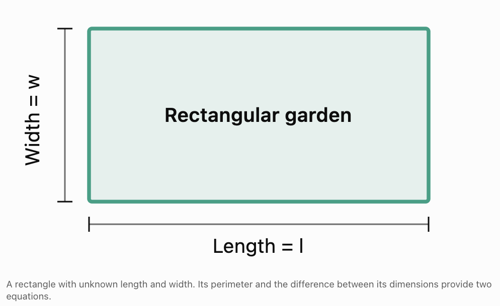
Step 1: Define variables
l = length of the garden, in metres
w = width of the garden, in metres
Step 2: Construct the perimeter equation
P = 2l + 2w
52 = 2l + 2w
Divide by 2:
l + w = 26
Step 3: Construct the second equation
The length is 6 m greater than the width.
l − w = 6
Step 4: Solve by elimination
l + w = 26
l − w = 6
Add:
2l = 32
l = 16
Substitute:
16 + w = 26
w = 10
Step 5: Verify
Perimeter:
2(16) + 2(10) = 52 m
Difference:
16 − 10 = 6 m
Both conditions are satisfied.
Answer: The garden is 16 m long and 10 m wide.
Geometric interpretation
The solution determines a unique rectangle satisfying both the perimeter and dimension conditions.
Its area is:
A = lw
A = 16(10)
A = 160 m²
The system provides dimensions that can be used for further calculations involving fencing, landscaping, or construction materials.
Application: Rectangle Dimensions from Area and Perimeter
Not all geometric systems are linear.
Suppose a rectangle has:
-
Perimeter = 34 cm.
-
Area = 60 cm².
Find its dimensions.
Step 1: Define variables
l = length, in cm
w = width, in cm
Step 2: Construct equations
Perimeter:
2l + 2w = 34
Simplify:
l + w = 17
Area:
lw = 60
Step 3: Substitute
From the perimeter equation:
l = 17 − w
Substitute into the area equation:
(17 − w)w = 60
17w − w² = 60
Rearrange:
w² − 17w + 60 = 0
Step 4: Factor
(w − 5)(w − 12) = 0
Therefore:
w = 5 or w = 12
If w = 5:
l = 12
If w = 12:
l = 5
These describe the same rectangle with its dimensions interchanged.
Answer: The rectangle measures 12 cm by 5 cm.
Verify
Perimeter:
2(12) + 2(5) = 34 cm
Area:
12(5) = 60 cm²
Important observation
The system contains a linear equation and a nonlinear equation.
Substitution transforms the system into a quadratic equation.
This demonstrates how systems of equations connect algebra and geometry.
Application: Finding Unknown Angles
Geometric angle relationships can be represented using systems of equations.
Worked Example: Complementary Angles
Two angles are complementary.
The larger angle is 18° greater than the smaller angle.
Find both angles.
Step 1: Define variables
x = larger angle, in degrees
y = smaller angle, in degrees
Step 2: Construct equations
Complementary angles add to 90°.
x + y = 90
The larger angle exceeds the smaller by 18°.
x − y = 18
Step 3: Solve
Add the equations:
2x = 108
x = 54
Then:
y = 90 − 54
y = 36
Step 4: Verify
54° + 36° = 90°
54° − 36° = 18°
Answer: The angles are 54° and 36°.
Application: Angles in a Triangle
The three interior angles of a triangle add to 180°.
Suppose:
-
The second angle is 20° greater than the first.
-
The third angle is twice the first.
Find all three angles.
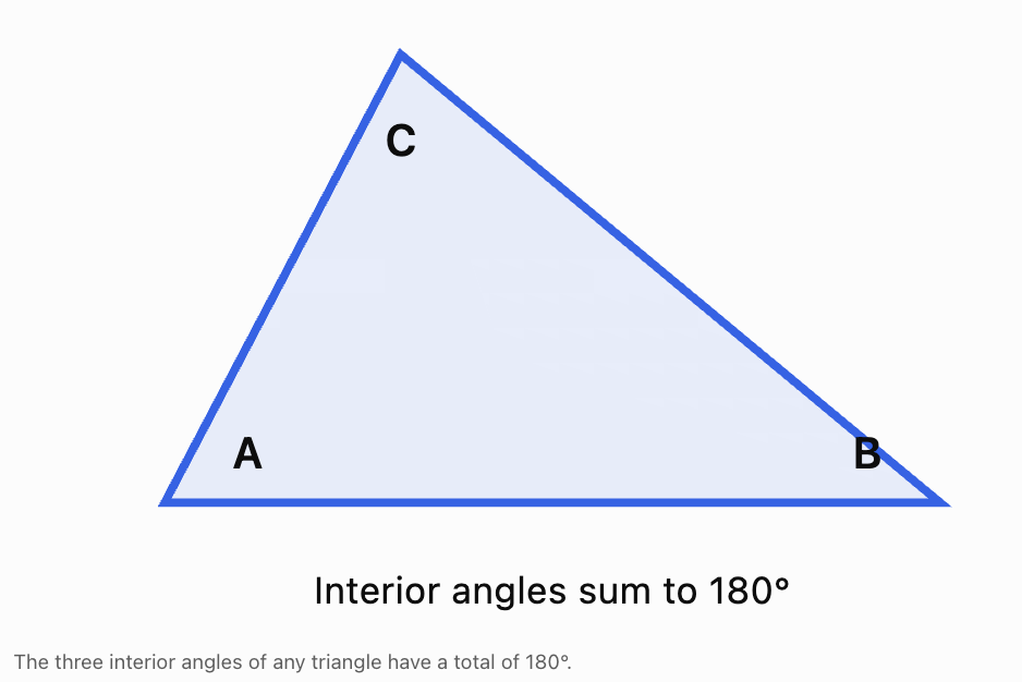
Step 1: Define variables
x = first angle
y = second angle
z = third angle
Step 2: Construct equations
Angle sum:
x + y + z = 180
Second angle relationship:
y = x + 20
Third angle relationship:
z = 2x
Step 3: Substitute
x + (x + 20) + 2x = 180
4x + 20 = 180
4x = 160
x = 40
Then:
y = 40 + 20 = 60
z = 2(40) = 80
Step 4: Verify
40° + 60° + 80° = 180°
60° − 40° = 20°
80° = 2(40°)
Answer: The triangle's angles are 40°, 60°, and 80°.
Geometric interpretation
All three angles are less than 90°, so the triangle is acute.
This example shows how a three-variable system can be solved efficiently using relationships between the variables.
Coordinate Geometry: Intersections of Straight Lines
In coordinate geometry, a straight line can be represented by an equation such as:
y = mx + b
where:
-
m = gradient or slope.
-
b = y-intercept.
-
x and y = coordinates of points on the line.
When two lines intersect, the intersection point satisfies both equations simultaneously.
Therefore, finding the intersection of two lines is equivalent to solving a system of equations.
Worked Example: Two Intersecting Lines
Find the intersection of:
y = 2x + 1
y = −x + 7
Step 1: Set the expressions equal
At the intersection, both equations have the same x-value and y-value.
2x + 1 = −x + 7
Step 2: Solve for x
3x = 6
x = 2
Step 3: Solve for y
y = 2(2) + 1
y = 5
Intersection: (2, 5).
Step 4: Verify
First equation:
5 = 2(2) + 1
Second equation:
5 = −2 + 7
Both are correct.
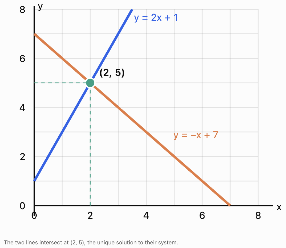
Geometric interpretation
The ordered pair (2, 5) represents a point that lies on both lines.
The x-coordinate is 2, and the y-coordinate is 5.
Because the lines have different gradients, they intersect at exactly one point.
Parallel and Coincident Lines
Not every pair of lines has one intersection.
Consider three possibilities.
|
Relationship |
Geometric meaning |
Number of solutions |
|---|---|---|
|
Intersecting lines |
Lines cross at one point |
One |
|
Distinct parallel lines |
Lines never meet |
None |
|
Coincident lines |
Both equations represent the same line |
Infinitely many |
Example: Parallel Lines
y = 3x + 2
y = 3x − 4
Setting the expressions equal:
3x + 2 = 3x − 4
2 = −4
This is impossible.
Conclusion: No solution.
Example: Coincident Lines
2x + 4y = 12
x + 2y = 6
Multiplying the second equation by 2 produces the first equation.
The equations represent the same line.
Conclusion: Infinitely many solutions.
Every point on that line satisfies both equations.
Application: Finding the Vertices of a Triangle
A triangle is formed by three lines:
Line A: y = x + 1
Line B: y = −x + 7
Line C: y = 2
Find the three vertices of the triangle.
Step 1: Find the intersection of A and B
x + 1 = −x + 7
2x = 6
x = 3
y = 4
First vertex:
P = (3, 4)
Step 2: Find the intersection of A and C
2 = x + 1
x = 1
Second vertex:
Q = (1, 2)
Step 3: Find the intersection of B and C
2 = −x + 7
x = 5
Third vertex:
R = (5, 2)
Step 4: Interpret geometrically
The vertices are:
P = (3, 4)
Q = (1, 2)
R = (5, 2)
Step 5: Calculate the area
The base QR lies horizontally along y = 2.
Its length is:
5 − 1 = 4 units
The vertical height from P to the base is:
4 − 2 = 2 units
Area of a triangle:
A = ½bh
A = ½(4)(2)
A = 4 square units
Verification
Check each vertex in its two corresponding line equations.
For P = (3, 4):
4 = 3 + 1
4 = −3 + 7
For Q = (1, 2):
2 = 1 + 1
2 = 2
For R = (5, 2):
2 = −5 + 7
2 = 2
All three vertices are correct.
Application: Finding the Intersection of a Line and a Circle
Systems can also contain nonlinear equations.
The equation of a circle with centre (h, k) and radius r is:
(x − h)² + (y − k)² = r²
Suppose we want to find where the line:
y = x + 1
intersects the circle:
x² + y² = 25
Step 1: Substitute the line equation
Replace y with x + 1:
x² + (x + 1)² = 25
Step 2: Expand
x² + x² + 2x + 1 = 25
2x² + 2x − 24 = 0
Divide by 2:
x² + x − 12 = 0
Step 3: Factor
(x + 4)(x − 3) = 0
Therefore:
x = −4 or x = 3
Step 4: Find the corresponding y-values
If x = −4:
y = −4 + 1 = −3
If x = 3:
y = 3 + 1 = 4
Intersection points: (−4, −3) and (3, 4).
Step 5: Verify
For (−4, −3):
Circle:
(−4)² + (−3)² = 16 + 9 = 25
Line:
−3 = −4 + 1
For (3, 4):
Circle:
3² + 4² = 9 + 16 = 25
Line:
4 = 3 + 1
Both points satisfy both equations.
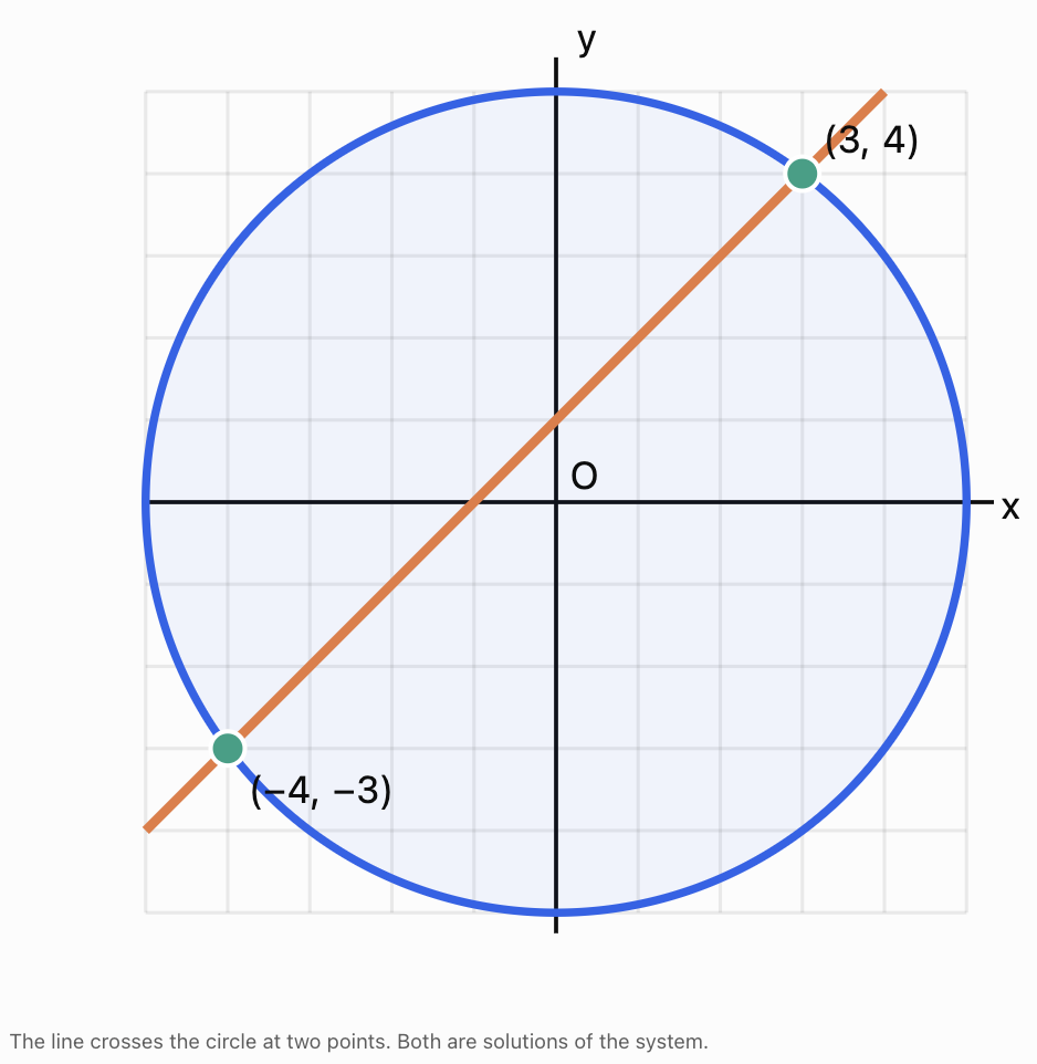
How many intersections are possible?
A straight line and a circle can have:
-
Two intersection points.
-
One intersection point, when the line is tangent.
-
No real intersection points.
The number of real solutions of the resulting quadratic equation determines the number of intersections.
Using the discriminant
For:
ax² + bx + c = 0
the discriminant is:
D = b² − 4ac
If:
-
D is positive: two distinct real intersections.
-
D = 0: one tangent intersection.
-
D is negative: no real intersections.
This provides a connection between quadratic equations and coordinate geometry.
Application: Finding an Unknown Point Using the Midpoint
The midpoint of a line segment lies halfway between its endpoints.
For endpoints A(x₁, y₁) and B(x₂, y₂), the midpoint is:
M = ((x₁ + x₂)/2, (y₁ + y₂)/2)
Suppose a line segment has:
A = (2, 4)
M = (5, 7)
Find the coordinates of B.
Step 1: Define the unknown endpoint
B = (x, y)
Step 2: Construct equations
For the x-coordinate:
(2 + x)/2 = 5
For the y-coordinate:
(4 + y)/2 = 7
Step 3: Solve
2 + x = 10
x = 8
4 + y = 14
y = 10
Answer: B = (8, 10).
Verify
Midpoint of (2, 4) and (8, 10):
M = ((2 + 8)/2, (4 + 10)/2)
M = (5, 7)
The calculated endpoint is correct.
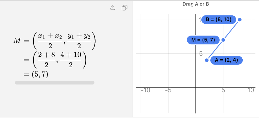
Geometric interpretation
The midpoint is exactly halfway between the endpoints in both coordinate directions.
The two coordinate equations can be solved independently because each involves a different unknown.
Application: Perpendicular Lines and Intersection Points
Two nonvertical lines are perpendicular when their gradients multiply to −1.
m₁m₂ = −1
Suppose a line passes through (2, 3) and has gradient 2.
Find the equation of the perpendicular line passing through (4, 1), and determine where the two lines intersect.
Step 1: Find the first line
Using point-slope form:
y − 3 = 2(x − 2)
y = 2x − 1
Step 2: Find the perpendicular gradient
The negative reciprocal of 2 is:
m = −1/2
Step 3: Find the second line
Through (4, 1):
y − 1 = −½(x − 4)
y = −½x + 3
Step 4: Solve the system
2x − 1 = −½x + 3
2.5x = 4
x = 8/5
Step 5: Find y
y = 2(8/5) − 1
y = 16/5 − 5/5
y = 11/5
Intersection: (8/5, 11/5).
Verify
First line:
2(8/5) − 1 = 11/5
Second line:
−½(8/5) + 3 = −4/5 + 15/5 = 11/5
Gradient product:
2(−1/2) = −1
Both the intersection and perpendicularity conditions are satisfied.
Geometric interpretation
The two lines meet at a right angle.
This method is useful when constructing perpendicular paths, locating perpendicular projections, or analysing geometric figures.
Application: Dimensions of a Rectangular Prism
Three-dimensional geometry can involve three unknown dimensions.
A rectangular storage box has:
-
Length + width + height = 24 cm.
-
Length is twice the width.
-
Height is 3 cm greater than the width.
Find the dimensions and volume.
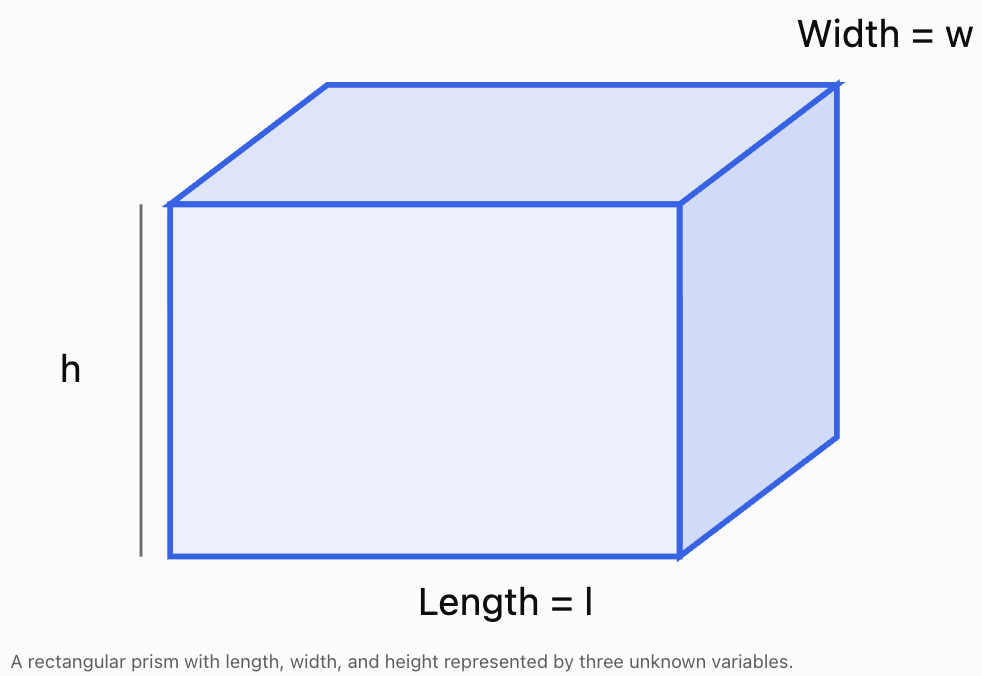
Step 1: Define variables
l = length, in cm
w = width, in cm
h = height, in cm
Step 2: Construct equations
l + w + h = 24
l = 2w
h = w + 3
Step 3: Substitute
2w + w + (w + 3) = 24
4w + 3 = 24
4w = 21
w = 21/4 = 5.25 cm
Step 4: Find the remaining dimensions
l = 2(5.25) = 10.5 cm
h = 5.25 + 3 = 8.25 cm
Step 5: Verify
10.5 + 5.25 + 8.25 = 24 cm
10.5 = 2(5.25)
8.25 = 5.25 + 3
All conditions are satisfied.
Step 6: Calculate volume
V = lwh
V = 10.5 × 5.25 × 8.25
V = 454.78125 cm³
Interpretation
The box measures:
-
Length: 10.5 cm.
-
Width: 5.25 cm.
-
Height: 8.25 cm.
Its volume is approximately 454.78 cm³.
This type of modelling is useful in packaging, storage design, and construction.
Applications in Design, Architecture, and Engineering
Systems of equations are used extensively when geometric conditions must be satisfied simultaneously.
Architecture
Determine room dimensions, wall intersections, and layouts that satisfy multiple design constraints.
Engineering
Calculate geometric intersections, structural dimensions, and positions of connected components.
Computer-Aided Design
Use equations to locate intersections and construct precise geometric models.
Land Surveying
Determine positions and boundaries from coordinate measurements and geometric relationships.
Example: Locating Two Paths
Two straight paths are modelled by:
Path A: y = 0.5x + 2
Path B: y = −x + 8
Their intersection is found by solving:
0.5x + 2 = −x + 8
1.5x = 6
x = 4
Then:
y = 0.5(4) + 2
y = 4
The paths intersect at (4, 4).
If the coordinates are measured in metres from a defined origin, the intersection is 4 m east and 4 m north of that origin, assuming positive x points east and positive y points north.
In a real design, the coordinate system and measurement units must be clearly defined.
Using Technology to Verify Geometric Solutions
Graphing calculators and mathematical software can help visualise geometric systems.
For example, enter:
y = 2x + 1
y = −x + 7
into Desmos Graphing Calculator.
The graph shows the lines intersecting at (2, 5).
For a line-circle system, enter:
x² + y² = 25
y = x + 1
The graph displays two intersection points.
Benefits of technology
Technology can:
-
Display geometric relationships visually.
-
Estimate intersection coordinates.
-
Check algebraic solutions.
-
Investigate the effect of changing parameters.
-
Help identify the number of intersections.
Limitations
Graphing technology may display approximate values.
A poorly chosen graphing window may hide intersections.
Some intersections may be difficult to identify accurately from the graph alone.
Therefore, algebraic verification remains important.
Evaluating Geometric Solutions
A solution may satisfy an equation but still be inappropriate for the geometric situation.
Positive dimensions
Lengths, widths, heights, radii, and areas cannot be negative in ordinary geometric measurement.
For example, a quadratic equation might produce:
w = 5 or w = −3
If w represents a physical width, the negative solution must be rejected.
Angle restrictions
Interior angles of a nondegenerate triangle must be greater than 0° and less than 180°.
Three proposed angles must also add to 180°.
Coordinate order
The point (3, 5) is different from (5, 3).
Coordinate order must be preserved.
Extraneous solutions
Squaring equations or performing other non-equivalent transformations may introduce solutions that do not satisfy the original system.
Every candidate solution should be checked.
Geometric assumptions
A drawing may not be to scale.
Do not assume two lines are perpendicular or two lengths are equal unless this is given or established mathematically.
Units
Lengths are measured in units such as cm or m.
Areas are measured in square units such as cm² or m².
Volumes are measured in cubic units such as cm³ or m³.
Using incorrect units can make an otherwise correct numerical result incomplete.
Common Mistakes
Using the wrong perimeter formula
For a rectangle:
P = 2l + 2w
not l + w.
Confusing area and perimeter
Area measures the region enclosed by a shape, while perimeter measures the distance around it.
Forgetting angle-sum relationships
Triangle angles add to 180°, while quadrilateral angles add to 360°.
Reversing coordinate values
The point (x, y) must be written in the correct order.
Assuming every system is linear
Area and circle equations often produce nonlinear systems.
Ignoring multiple solutions
A line may intersect a circle at two points.
Both points must be included when valid.
Accepting negative dimensions
Negative lengths or widths are not valid physical dimensions.
Assuming a diagram is drawn to scale
Only use relationships given or justified by geometry.
Misinterpreting parallel lines
Parallel lines with different intercepts have no intersection.
Forgetting to verify intersections
A coordinate must satisfy both equations to be an intersection point.
Using incorrect units
Lengths, areas, and volumes require different types of units.
Relying only on graphing technology
Graphical answers may be approximate or incomplete.
Key Terms
-
System of equations: Two or more equations solved simultaneously.
-
Coordinate geometry: The study of geometric figures using coordinates and equations.
-
Cartesian plane: A coordinate plane with perpendicular x- and y-axes.
-
Ordered pair: A pair of coordinates written as (x, y).
-
Intersection point: A point shared by two or more geometric objects.
-
Gradient: The slope of a straight line.
-
Y-intercept: The point where a line crosses the y-axis.
-
Parallel lines: Coplanar lines that never intersect.
-
Perpendicular lines: Lines that meet at a right angle.
-
Coincident lines: Lines that occupy exactly the same position.
-
Perimeter: The total distance around a shape.
-
Area: The amount of two-dimensional space enclosed by a shape.
-
Volume: The amount of three-dimensional space occupied by an object.
-
Complementary angles: Two angles whose sum is 90°.
-
Supplementary angles: Two angles whose sum is 180°.
-
Midpoint: The point halfway between two endpoints.
-
Circle: The set of points at a fixed distance from a centre.
-
Radius: The distance from the centre of a circle to its boundary.
-
Tangent: A line that touches a circle at exactly one point.
-
Discriminant: The expression b² − 4ac, which helps determine the number of real roots of a quadratic equation.
-
Nonlinear system: A system containing at least one nonlinear equation.
-
Extraneous solution: A solution introduced during algebraic manipulation that does not satisfy the original problem.
-
Geometric constraint: A condition restricting possible dimensions, angles, or positions.
-
Verification: Checking that a solution satisfies the original equations and geometric conditions.
Key Takeaways
-
Systems of equations can model lengths, widths, angles, coordinates, and dimensions.
-
Geometric properties provide relationships that can be expressed as equations.
-
Rectangle problems may involve perimeter, area, and dimension relationships.
-
Angle problems can use triangle angle sums and relationships between angles.
-
The intersection of two lines is a solution common to both line equations.
-
Parallel lines have no intersection, while coincident lines have infinitely many shared points.
-
Triangle vertices can be found by solving pairs of line equations.
-
A line and a circle may have zero, one, or two real intersection points.
-
Midpoint relationships can be used to find unknown coordinates.
-
Three-variable systems can determine the dimensions of three-dimensional objects.
-
Geometric solutions must satisfy relevant restrictions and use correct units.
-
Verification is essential for confirming that calculated values represent valid geometric results.
Check Your Understanding
Recall and Understanding
1. Explain how a system of equations can be used to determine the dimensions of a rectangle.
2. What does the solution to a system of two straight-line equations represent geometrically?
3. Explain the difference between intersecting, parallel, and coincident lines.
4. Why might a line-circle system have two solutions?
5. Why must negative solutions sometimes be rejected in geometric problems?
Rectangle and Angle Problems
6. A rectangle has a perimeter of 48 cm.
Its length is 8 cm greater than its width.
Find its dimensions and area.
7. A rectangle has a perimeter of 30 cm and an area of 54 cm².
Find its dimensions.
8. Two complementary angles differ by 24°.
Find both angles.
9. The second angle of a triangle is 15° greater than the first.
The third angle is twice the first.
Find all three angles.
10. Three angles of a quadrilateral are x, x + 20°, and 2x. The fourth angle is 100°.
Find all four angles.
Coordinate Geometry
11. Find the intersection of:
y = 3x − 2
y = −x + 10
12. Determine the number of solutions:
y = 4x + 3
y = 4x − 7
13. Determine the number of solutions:
2x + 6y = 18
x + 3y = 9
14. Find the vertices of the triangle formed by:
y = x
y = −x + 6
y = 1
15. Find the intersection points of:
x² + y² = 25
y = 3
Applications and Challenge
16. A line segment has endpoint A = (3, 5) and midpoint M = (7, 9).
Find the other endpoint.
17. A line has gradient 3 and passes through (1, 2).
Find the equation of the perpendicular line passing through (4, 5), then determine the intersection of the two lines.
18. A rectangular prism has length, width, and height whose sum is 30 cm.
The length is twice the width.
The height is 6 cm greater than the width.
Find its dimensions and volume.
19. Find the intersection points of:
y = x + 2
x² + y² = 20
20. A rectangular garden has a perimeter of 60 m and an area of 200 m².
Find its dimensions and explain how you verify the result.
Answers to Check Your Understanding
1. Rectangle dimensions
Define variables for length and width.
Use geometric information, such as perimeter and a relationship between the dimensions, to construct two equations.
Solve the system and verify that the dimensions satisfy the original conditions.
2. Intersection of two lines
The solution represents the coordinates of a point lying on both lines.
For example, (3, 5) means both lines pass through x = 3, y = 5.
3. Types of lines
Intersecting lines cross at one point and have one solution.
Distinct parallel lines never meet and have no solution.
Coincident lines represent the same line and have infinitely many solutions.
4. Line-circle intersections
A line can pass through a circle at two different points.
Both intersection points satisfy the line equation and circle equation.
The resulting quadratic equation may therefore have two distinct real solutions.
5. Negative geometric values
Physical dimensions such as lengths, widths, and radii cannot be negative.
Therefore, a negative algebraic solution must be rejected when it represents an invalid dimension.
Negative coordinates, however, can be perfectly valid.
6. Rectangle perimeter
Let:
l = length
w = width
Perimeter:
2l + 2w = 48
l + w = 24
Difference:
l − w = 8
Add:
2l = 32
l = 16
Then:
w = 8
Area:
A = 16(8) = 128 cm²
Answer: Length = 16 cm, width = 8 cm, area = 128 cm².
7. Rectangle area and perimeter
Perimeter:
2l + 2w = 30
l + w = 15
Area:
lw = 54
Substitute l = 15 − w:
(15 − w)w = 54
15w − w² = 54
w² − 15w + 54 = 0
(w − 6)(w − 9) = 0
Therefore:
w = 6 or w = 9
Answer: The rectangle measures 9 cm by 6 cm.
Verification:
2(9) + 2(6) = 30 cm
9(6) = 54 cm²
8. Complementary angles
Let:
x = larger angle
y = smaller angle
Equations:
x + y = 90
x − y = 24
Add:
2x = 114
x = 57
Then:
y = 33
Answer: 57° and 33°.
9. Triangle angles
Let the first angle be x.
Second angle:
x + 15
Third angle:
2x
Angle sum:
x + (x + 15) + 2x = 180
4x + 15 = 180
4x = 165
x = 41.25
Second angle:
56.25°
Third angle:
82.5°
Answer: 41.25°, 56.25°, and 82.5°.
Verification:
41.25 + 56.25 + 82.5 = 180°
10. Quadrilateral angles
Angle sum:
x + (x + 20) + 2x + 100 = 360
4x + 120 = 360
4x = 240
x = 60
Therefore:
First angle = 60°
Second angle = 80°
Third angle = 120°
Fourth angle = 100°
Answer: 60°, 80°, 120°, and 100°.
Verification:
60 + 80 + 120 + 100 = 360°
11. Intersection of two lines
Equations:
y = 3x − 2
y = −x + 10
Set equal:
3x − 2 = −x + 10
4x = 12
x = 3
Then:
y = 3(3) − 2 = 7
Answer: (3, 7).
Verification:
7 = −3 + 10
12. Parallel lines
Equations:
y = 4x + 3
y = 4x − 7
Both lines have gradient 4 but different y-intercepts.
Answer: No solution.
13. Coincident lines
Equations:
2x + 6y = 18
x + 3y = 9
Multiplying the second equation by 2 gives the first.
Answer: Infinitely many solutions.
14. Triangle vertices
Lines:
y = x
y = −x + 6
y = 1
First intersection:
x = −x + 6
2x = 6
x = 3
y = 3
First vertex: (3, 3)
Second intersection:
1 = x
Second vertex: (1, 1)
Third intersection:
1 = −x + 6
x = 5
Third vertex: (5, 1)
Answer: (3, 3), (1, 1), and (5, 1).
15. Line-circle intersections
Circle:
x² + y² = 25
Line:
y = 3
Substitute:
x² + 3² = 25
x² + 9 = 25
x² = 16
x = ±4
Answer: (−4, 3) and (4, 3).
Verification:
16 + 9 = 25 for both points.
16. Unknown endpoint
Given:
A = (3, 5)
M = (7, 9)
Let the other endpoint be B = (x, y).
Midpoint equations:
(3 + x)/2 = 7
(5 + y)/2 = 9
Solve:
3 + x = 14
x = 11
5 + y = 18
y = 13
Answer: B = (11, 13).
17. Perpendicular lines
The first line has gradient 3 and passes through (1, 2).
Using point-slope form:
y − 2 = 3(x − 1)
y = 3x − 1
The perpendicular gradient is:
−1/3
Through (4, 5):
y − 5 = −⅓(x − 4)
y = −x/3 + 19/3
Find the intersection:
3x − 1 = −x/3 + 19/3
Multiply by 3:
9x − 3 = −x + 19
10x = 22
x = 11/5
Substitute:
y = 3(11/5) − 1
y = 28/5
Answer: The perpendicular line is y = −x/3 + 19/3, and the intersection is (11/5, 28/5).
Verification:
3(−1/3) = −1
The gradients confirm that the lines are perpendicular.
18. Rectangular prism
Let:
l = length
w = width
h = height
Equations:
l + w + h = 30
l = 2w
h = w + 6
Substitute:
2w + w + (w + 6) = 30
4w + 6 = 30
4w = 24
w = 6
Then:
l = 12
h = 12
Volume:
V = lwh
V = 12(6)(12)
V = 864 cm³
Answer: Length = 12 cm, width = 6 cm, height = 12 cm, volume = 864 cm³.
19. Line-circle intersections
Given:
y = x + 2
x² + y² = 20
Substitute:
x² + (x + 2)² = 20
Expand:
x² + x² + 4x + 4 = 20
2x² + 4x − 16 = 0
Divide by 2:
x² + 2x − 8 = 0
Factor:
(x + 4)(x − 2) = 0
Therefore:
x = −4 or x = 2
If x = −4:
y = −2
If x = 2:
y = 4
Answer: (−4, −2) and (2, 4).
Verification:
For (−4, −2):
16 + 4 = 20
For (2, 4):
4 + 16 = 20
Both points also satisfy y = x + 2.
20. Rectangular garden
Given:
Perimeter = 60 m
Area = 200 m²
Let:
l = length
w = width
Perimeter:
2l + 2w = 60
l + w = 30
Area:
lw = 200
Substitute:
l = 30 − w
(30 − w)w = 200
30w − w² = 200
w² − 30w + 200 = 0
Factor:
(w − 10)(w − 20) = 0
Therefore:
w = 10 or w = 20
The dimensions are interchangeable.
Answer: The garden measures 20 m by 10 m.
Verification:
Perimeter:
2(20) + 2(10) = 60 m
Area:
20(10) = 200 m²
Both original conditions are satisfied.
Final Summary
Systems of equations provide a powerful connection between algebra and geometry. They allow us to determine unknown dimensions, calculate angles, find intersections, locate vertices, and analyse geometric figures in two and three dimensions.
Some geometric systems are linear, while others involve quadratic equations or additional geometric relationships.
The most important part of solving these problems is constructing equations that accurately represent the geometric conditions.
Once a solution has been obtained, it should be verified using the original equations, relevant geometric properties, and appropriate units.
Successful geometric problem-solving combines algebraic accuracy, visual understanding, and careful interpretation of mathematical results.
4. Mathematical Modelling
Learning outcomes
- I can create mathematical models using systems of equations.
- I can identify assumptions in a model.
- I can solve models using appropriate methods.
- I can interpret solutions in real-world contexts.
- I can evaluate how well a model represents reality.
Introduction
Mathematics is more than a collection of equations and calculations. It is a powerful tool for understanding the world, making predictions, solving practical problems, and supporting decisions.
Scientists use mathematics to describe motion and chemical reactions. Businesses use it to analyse costs and profits. Engineers use it to design structures. Environmental researchers use it to investigate pollution, energy consumption, and resource use.
In many of these situations, several unknown quantities are connected by different relationships. Systems of equations allow us to represent these relationships mathematically and investigate how they interact.
The process of converting a real-world situation into mathematical relationships is called mathematical modelling.
A mathematical model is not necessarily an exact description of reality. Instead, it is a simplified representation that focuses on the most important features of a situation.
A good mathematical model should be:
-
Based on relevant information.
-
Mathematically consistent.
-
Appropriate for the situation.
-
Clear about its assumptions.
-
Useful for answering a particular question.
-
Tested against real-world evidence when possible.
In this topic, we will explore how to construct systems-based models, solve them, interpret their results, and evaluate how well they represent reality.
What Is Mathematical Modelling?
Mathematical modelling is the process of representing a real-world situation using mathematical ideas, relationships, and equations.
A model may involve:
-
Variables representing unknown quantities.
-
Equations describing relationships.
-
Constants representing known values.
-
Constraints restricting possible solutions.
-
Assumptions that simplify the situation.
For example, suppose a company manufactures two products.
Let:
x = number of Product A units.
y = number of Product B units.
The company produces 200 units in total.
This gives:
x + y = 200
Product A requires 2 hours of labour, while Product B requires 3 hours.
The company uses 480 labour-hours.
This gives:
2x + 3y = 480
Together, these equations form a mathematical model of the production situation.
The system is:
x + y = 200
2x + 3y = 480
Solving the system determines the production quantities.
Solving the introductory model
Multiply the first equation by 2:
2x + 2y = 400
Subtract this from the second equation:
y = 80
Substitute:
x + 80 = 200
x = 120
Answer: The company manufactures 120 units of Product A and 80 units of Product B.
Verification:
120 + 80 = 200 units
2(120) + 3(80) = 480 labour-hours
The model is mathematically consistent.
However, its usefulness depends on whether the labour requirements and production totals accurately represent the real situation.
The Mathematical Modelling Cycle
Mathematical modelling is not simply a process of writing equations and calculating answers.
It is a cycle involving interpretation, testing, and improvement.
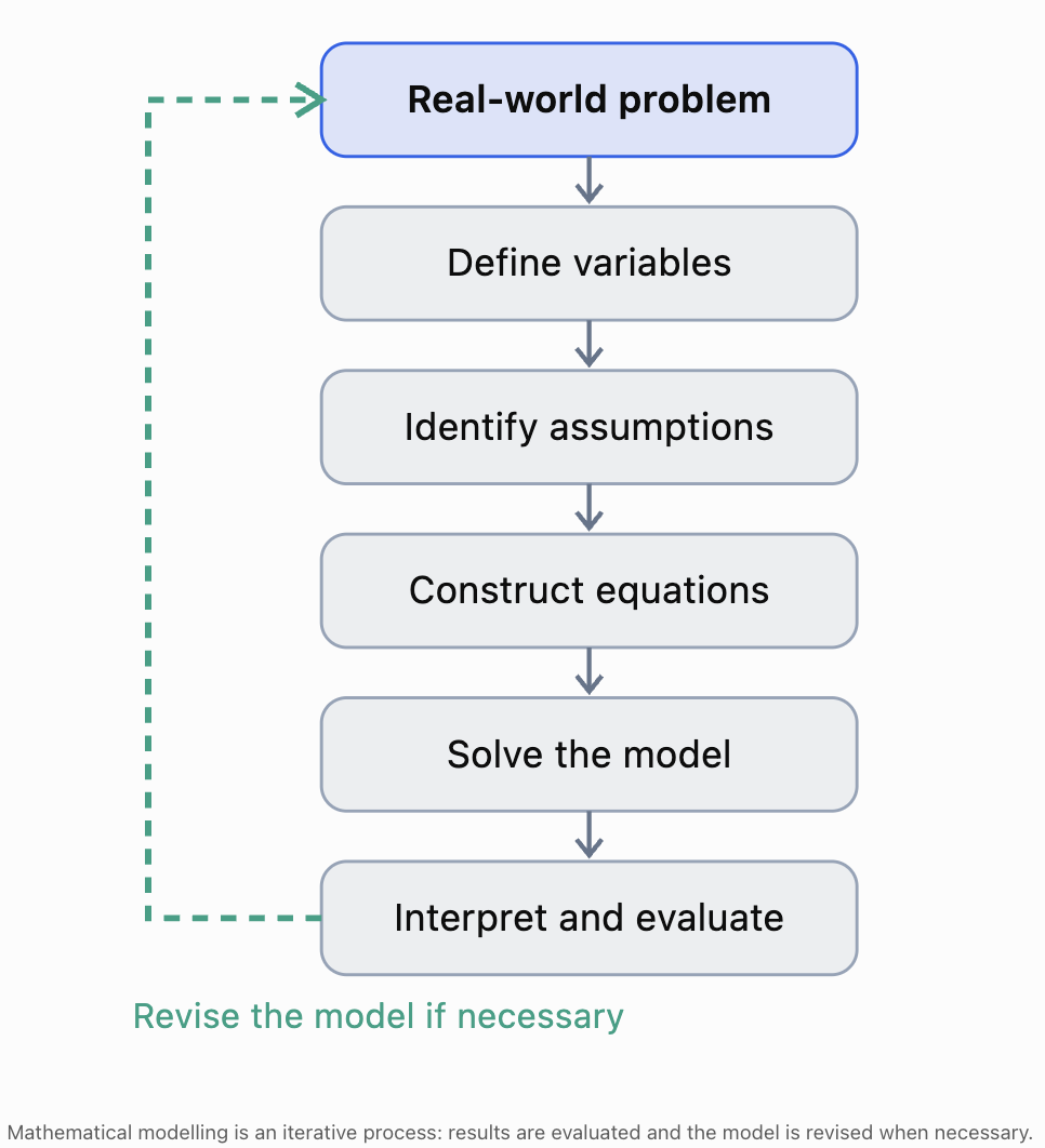
Understanding the stages
Real-world problem: Identify what needs to be investigated or decided.
Define variables: Represent unknown quantities with suitable symbols.
Identify assumptions: Decide which features of reality can be simplified.
Construct equations: Translate the available information into mathematical relationships.
Solve the model: Use algebraic, graphical, numerical, or technological methods.
Interpret and evaluate: Explain the results, check them against reality, and determine whether the model should be improved.
The final stage is particularly important.
A model may produce a mathematically correct solution that is unrealistic or unsuitable for the original problem.
Variables, Parameters, and Constraints
Three important components of mathematical models are variables, parameters, and constraints.
Variables
A variable represents a quantity that can change or an unknown value.
Examples:
x = number of products sold
t = time, in seconds
v = velocity, in m/s
Parameters
A parameter is a value that defines a particular model.
For example:
C = 500 + 8x
Here:
-
C is total cost.
-
x is production quantity.
-
500 is the fixed cost.
-
8 is the variable cost per unit.
The numbers 500 and 8 are parameters of the cost model.
They may change if the business conditions change.
Constraints
A constraint restricts which solutions are acceptable.
For example, if x represents the number of products manufactured:
x ≥ 0
If products must be complete units:
x must be a whole number.
If a factory can produce at most 300 units:
x ≤ 300
Constraints are important because a mathematical system may produce solutions that are not realistic.
Example
A factory model produces:
x = 125.5
y = 74.5
These values may satisfy the equations.
However, if x and y represent complete manufactured products, the solution is not physically possible as an exact production plan.
The model may need to be adjusted or solved using integer constraints.
Identifying Assumptions in Mathematical Models
An assumption is a condition accepted as true for the purpose of constructing or using a model.
Assumptions simplify complex situations.
For example, a model of vehicle motion may assume that speed remains constant.
A business model may assume that selling price does not change.
A mixture model may assume that volumes are additive.
Common assumptions
|
Situation |
Possible assumption |
|---|---|
|
Business costs |
Variable cost per unit is constant |
|
Sales revenue |
All products sell at the same price |
|
Motion |
Objects travel at constant speeds |
|
Chemical mixtures |
Volumes are additive |
|
Electricity |
Resistance remains constant |
|
Population studies |
The population is closed |
|
Manufacturing |
Each unit requires the same resources |
|
Geometry |
Measurements and shapes are exact |
Why assumptions matter
Assumptions make mathematical modelling manageable, but they also limit how accurately a model represents reality.
For example, consider:
C = 1000 + 5x
This model assumes that fixed costs remain $1,000 and variable costs remain $5 per unit.
However, producing more units might require a second factory shift, additional equipment, or overtime pay.
The original model may no longer be accurate beyond a certain production level.
A good mathematical conclusion should explain the assumptions on which the result depends.
Worked Example: Modelling a School Event
A school sells adult and student tickets for a performance.
Adult tickets cost $15.
Student tickets cost $10.
A total of 200 tickets are sold.
Total revenue is $2,400.
Determine the number of adult and student tickets sold.
Step 1: Identify the unknowns
Let:
a = number of adult tickets
s = number of student tickets
Step 2: Identify assumptions
Assume:
-
Every ticket sold is either an adult or student ticket.
-
Adult tickets all cost $15.
-
Student tickets all cost $10.
-
There are no refunds or discounts.
-
Revenue includes only ticket sales.
Step 3: Construct the equations
Total tickets:
a + s = 200
Total revenue:
15a + 10s = 2400
Step 4: Solve by elimination
Multiply the first equation by 10:
10a + 10s = 2000
Subtract from the revenue equation:
5a = 400
a = 80
Then:
s = 200 − 80
s = 120
Step 5: Interpret
80 adult tickets were sold.
120 student tickets were sold.
Step 6: Verify
Total tickets:
80 + 120 = 200
Revenue:
15(80) + 10(120)
= 1200 + 1200
= $2400
Answer: 80 adult tickets and 120 student tickets.
Step 7: Evaluate the model
The result is reasonable because:
-
Both quantities are nonnegative.
-
Both quantities are whole numbers.
-
The total number of tickets is correct.
-
The revenue matches the recorded amount.
However, if discounted tickets or complimentary admissions were included, the model might need additional variables.
Worked Example: Modelling Production and Resource Use
A small factory manufactures tables and chairs.
Each table requires:
-
5 hours of labour.
-
4 units of wood.
Each chair requires:
-
2 hours of labour.
-
3 units of wood.
During one production period, the factory uses:
-
90 labour-hours.
-
80 units of wood.
Determine the number of tables and chairs produced.
Step 1: Define variables
t = number of tables
c = number of chairs
Step 2: Construct the equations
Labour:
5t + 2c = 90
Wood:
4t + 3c = 80
Step 3: Solve by elimination
Multiply the first equation by 3:
15t + 6c = 270
Multiply the second equation by 2:
8t + 6c = 160
Subtract:
7t = 110
t = 110/7 ≈ 15.714
Substitute into the first equation:
5(110/7) + 2c = 90
550/7 + 2c = 630/7
2c = 80/7
c = 40/7 ≈ 5.714
Step 4: Interpret
The system produces:
t ≈ 15.714 tables
c ≈ 5.714 chairs
These quantities are mathematically valid but not realistic for complete furniture products.
Step 5: Evaluate
The model assumes that both recorded resource totals were used entirely to manufacture complete tables and chairs.
Because the solution contains fractional quantities, the recorded totals and assumptions cannot all describe a production plan consisting only of complete items.
Step 6: Improve the model
Possible explanations include:
-
Some materials were wasted.
-
Some labour-hours were used for other activities.
-
Resource measurements were rounded.
-
Production requirements vary between individual products.
If the factory is planning future production rather than reconstructing past production, it may be more appropriate to use inequalities:
5t + 2c ≤ 90
4t + 3c ≤ 80
t ≥ 0, c ≥ 0
with t and c restricted to whole numbers.
This changes the task from solving an exact system to finding a feasible production plan.
Important lesson: A mathematical model may reveal that the original assumptions are too restrictive or that the data are inconsistent with the intended interpretation.
Improving a Model with Realistic Data
Consider a revised production example.
A factory manufactures tables and chairs.
Each table requires 5 labour-hours and 4 units of wood.
Each chair requires 2 labour-hours and 3 units of wood.
The factory uses:
-
70 labour-hours.
-
60 units of wood.
The model becomes:
5t + 2c = 70
4t + 3c = 60
Multiply the first equation by 3:
15t + 6c = 210
Multiply the second equation by 2:
8t + 6c = 120
Subtract:
7t = 90
t = 90/7
This still produces a fractional solution.
This tells us that changing the totals does not automatically produce a feasible integer solution.
A better approach is to choose a feasible production plan and calculate its resource requirements.
Suppose the factory produces:
t = 10 tables
c = 15 chairs
Then:
Labour:
5(10) + 2(15) = 80 hours
Wood:
4(10) + 3(15) = 85 units
A consistent model is therefore:
5t + 2c = 80
4t + 3c = 85
Solving this system gives:
t = 10, c = 15
This illustrates how mathematical models can be checked against feasible real-world scenarios.
Worked Example: Modelling Travel and Motion
Two vehicles leave the same location at the same time and travel in opposite directions.
After 4 hours, they are 320 km apart.
The faster vehicle travels 20 km/h faster than the slower vehicle.
Find their speeds.
Step 1: Define variables
x = speed of slower vehicle, in km/h
y = speed of faster vehicle, in km/h
Step 2: Identify assumptions
Assume:
-
Both vehicles maintain constant speeds.
-
They travel in opposite directions along a straight route.
-
They begin at the same time.
-
Neither vehicle stops.
Step 3: Construct equations
Distance = speed × time
Combined separation:
4x + 4y = 320
Simplify:
x + y = 80
Speed difference:
y − x = 20
Step 4: Solve
Add the equations:
2y = 100
y = 50
Then:
x = 30
Step 5: Interpret
Slower vehicle = 30 km/h
Faster vehicle = 50 km/h
Step 6: Verify
Distances:
30(4) = 120 km
50(4) = 200 km
Combined separation:
120 + 200 = 320 km
Speed difference:
50 − 30 = 20 km/h
Answer: The vehicles travel at 30 km/h and 50 km/h.
Step 7: Evaluate
The model is appropriate if the vehicles travel at approximately constant speeds.
If the vehicles accelerate, stop, or follow curved routes, a more complex model may be required.
Worked Example: Modelling a Chemical Mixture
A laboratory needs 500 mL of a 20% solution.
It has:
-
A 10% solution.
-
A 30% solution.
Determine the volume of each solution required.
Step 1: Define variables
x = volume of 10% solution, in mL
y = volume of 30% solution, in mL
Step 2: Identify assumptions
Assume:
-
The concentration percentages use the same definition.
-
Volumes are additive.
-
No solute is lost during mixing.
-
The solutions are mixed completely.
Step 3: Construct equations
Total volume:
x + y = 500
Solute-equivalent volume:
0.10x + 0.30y = 0.20(500)
Simplify:
0.10x + 0.30y = 100
Step 4: Solve
From the first equation:
x = 500 − y
Substitute:
0.10(500 − y) + 0.30y = 100
50 − 0.10y + 0.30y = 100
0.20y = 50
y = 250
Then:
x = 250
Step 5: Verify
Total volume:
250 + 250 = 500 mL
Solute-equivalent volume:
0.10(250) + 0.30(250)
= 25 + 75
= 100 mL
Final concentration:
100/500 × 100% = 20%
Answer: 250 mL of each solution.
Step 6: Evaluate
The result is valid under the stated assumptions.
For precise laboratory work, volume changes during mixing and the definition of concentration may need to be considered.
Worked Example: Comparing Two Cost Models
A business is considering two equipment rental plans.
Plan A:
$500 fixed charge plus $20 per hour.
Plan B:
$200 fixed charge plus $35 per hour.
At how many hours do the plans cost the same?
Step 1: Define variables
h = number of rental hours
C = total rental cost, in dollars
Step 2: Construct equations
Plan A:
C = 500 + 20h
Plan B:
C = 200 + 35h
Step 3: Solve
500 + 20h = 200 + 35h
300 = 15h
h = 20
Step 4: Calculate the cost
Plan A:
C = 500 + 20(20) = $900
Plan B:
C = 200 + 35(20) = $900
Answer: Both plans cost $900 for 20 hours of rental.
Step 5: Interpret
For fewer than 20 hours, Plan B is cheaper.
For more than 20 hours, Plan A is cheaper.
At exactly 20 hours, the costs are equal.
Step 6: Evaluate
The model assumes that both plans charge according to the stated rates.
It ignores taxes, discounts, minimum rental periods, and additional fees.
These factors could affect the actual cost comparison.
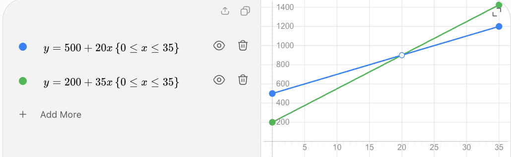
The two cost models intersect at 20 hours and $900. The graph represents the simplified pricing assumptions.
Choosing an Appropriate Method to Solve a Model
Different mathematical models may be easier to solve using different methods.
Substitution
Substitution is useful when one variable is already isolated or can be isolated easily.
Example:
x + y = 50
y = 2x + 5
Substitute the second equation into the first.
Elimination
Elimination is useful when coefficients can be made equal or opposite.
Example:
3x + 2y = 40
5x − 2y = 24
Adding the equations eliminates y.
Graphing
Graphing is useful when the model involves two variables and the intersection has a meaningful interpretation.
For example, cost and revenue models can be graphed to identify a break-even point.
Matrix methods
Matrix methods are useful for larger systems involving three or more variables.
A system such as:
2x + y + z = 12
x + 3y + 2z = 17
3x + 2y + 4z = 25
can be represented in matrix form:
A𝐱 = 𝐛
where A contains the coefficients, 𝐱 contains the unknowns, and 𝐛 contains the constants.
Technology
Graphing calculators, spreadsheets, and mathematical software are useful when:
-
Systems contain many variables.
-
Coefficients are complicated.
-
Several scenarios must be compared.
-
Models need to be updated frequently.
-
Experimental data must be analysed.
However, technology does not replace the need to understand the assumptions and meaning of a model.
Modelling with Three Variables
Some situations require three or more unknown quantities.
Worked Example: A School Fundraising Sale
A school sells three products:
-
Notebooks for $5.
-
Water bottles for $10.
-
T-shirts for $15.
A total of 100 products are sold.
Total revenue is $900.
The number of notebooks sold is twice the number of T-shirts sold.
Find the quantity of each product.
Step 1: Define variables
n = number of notebooks
w = number of water bottles
t = number of T-shirts
Step 2: Construct equations
Total quantity:
n + w + t = 100
Total revenue:
5n + 10w + 15t = 900
Quantity relationship:
n = 2t
Step 3: Substitute
From the third equation:
n = 2t
Substitute into the quantity equation:
2t + w + t = 100
w + 3t = 100
Therefore:
w = 100 − 3t
Substitute into the revenue equation:
5(2t) + 10(100 − 3t) + 15t = 900
10t + 1000 − 30t + 15t = 900
1000 − 5t = 900
−5t = −100
t = 20
Then:
n = 2(20) = 40
w = 100 − 3(20) = 40
Step 4: Interpret
Notebooks: 40
Water bottles: 40
T-shirts: 20
Step 5: Verify
Total quantity:
40 + 40 + 20 = 100
Revenue:
5(40) + 10(40) + 15(20)
= 200 + 400 + 300
= $900
Quantity relationship:
40 = 2(20)
Answer: 40 notebooks, 40 water bottles, and 20 T-shirts.
Step 6: Evaluate
The model assumes constant prices and that the revenue comes only from these three products.
The result is reasonable because all quantities are nonnegative whole numbers and satisfy every condition.
Models with No Solution or Infinitely Many Solutions
Not every system has a unique solution.
No solution
Consider:
x + y = 100
x + y = 120
These equations cannot both be true.
The model is inconsistent.
In a real-world situation, this may indicate incorrect data, incompatible measurements, or an unsuitable assumption.
Infinitely many solutions
Consider:
x + y = 100
2x + 2y = 200
The second equation provides no new information.
Many pairs of values satisfy both equations.
The model is underdetermined.
Additional independent information is needed to determine a unique solution.
Why this matters
A mathematical model may fail to determine a unique answer because the available information is insufficient.
Recognising this limitation is an important part of modelling.
Evaluating How Well a Model Represents Reality
A mathematical model should be evaluated using more than mathematical correctness.
Accuracy
Does the model reproduce observed measurements?
For example, if a model predicts 100 units sold but the business records only 70, the model may need revision.
Reasonableness
Are the calculated values realistic?
A model predicting negative production quantities is usually inappropriate for a physical manufacturing situation.
Assumptions
Are the simplifying assumptions valid?
A constant-speed model may be unsuitable for a vehicle that accelerates and brakes frequently.
Sensitivity
How much do the results change when the inputs change?
If a small change in measurement produces a large change in the solution, the model may be sensitive to uncertainty.
Range of validity
Does the model remain accurate over the range where it is being used?
A linear cost model may be accurate for 100–500 units but inaccurate for 10,000 units.
Predictive usefulness
Can the model make reliable predictions about situations not used to construct it?
A model that matches past data perfectly may still perform poorly when predicting future outcomes.
Practical constraints
Does the solution satisfy real-world restrictions?
Examples include:
-
Production capacity.
-
Available resources.
-
Nonnegative quantities.
-
Whole-number requirements.
-
Maximum speed or force limits.
-
Financial budgets.
Sensitivity Analysis
Sensitivity analysis investigates how changes in the assumptions or parameters affect the solution.
Consider the equipment rental models:
Plan A:
Cₐ = 500 + 20h
Plan B:
Cᵦ = 200 + 35h
The equal-cost point is 20 hours.
Now suppose Plan B increases its hourly rate from $35 to $40.
The revised equation is:
Cᵦ = 200 + 40h
Set the costs equal:
500 + 20h = 200 + 40h
300 = 20h
h = 15
The equal-cost point changes from 20 hours to 15 hours.
Interpretation
Increasing Plan B's hourly rate makes Plan A more competitive at a lower rental duration.
This illustrates how a change in one model parameter can affect the final decision.
Comparison
|
Plan B hourly rate |
Equal-cost rental duration |
|---|---|
|
$30 |
30 hours |
|
$35 |
20 hours |
|
$40 |
15 hours |
|
$45 |
12 hours |
The model can be used to investigate different pricing scenarios before making a decision.
Model Validation and Experimental Data
A model is validated by comparing its predictions with observations or independent data.
Suppose a scientist models the position of an object using:
s = 4t + 2
where:
-
s = position, in metres.
-
t = time, in seconds.
The model predicts:
|
Time (s) |
Predicted position (m) |
|---|---|
|
0 |
2 |
|
1 |
6 |
|
2 |
10 |
|
3 |
14 |
|
4 |
18 |
Suppose the actual measurements are:
|
Time (s) |
Measured position (m) |
|---|---|
|
0 |
2.1 |
|
1 |
5.9 |
|
2 |
10.2 |
|
3 |
13.8 |
|
4 |
18.1 |
The measurements are close to the predictions.
This suggests that the linear model may be appropriate over the observed time interval.
However, additional measurements would be needed to determine whether the model remains accurate over longer periods.
Residuals
A residual is the difference between an observed value and a predicted value.
Residual = observed value − predicted value
At t = 2 s:
Residual = 10.2 − 10
Residual = +0.2 m
At t = 3 s:
Residual = 13.8 − 14
Residual = −0.2 m
Small residuals suggest that the model closely matches the measurements.
However, the pattern of residuals is also important.
A systematic pattern may indicate that the model is missing an important relationship.
Improving Mathematical Models
A model can be improved by:
-
Collecting more accurate data.
-
Adding relevant variables.
-
Revising unrealistic assumptions.
-
Including important constraints.
-
Using a nonlinear relationship when necessary.
-
Comparing predictions with independent observations.
-
Considering measurement uncertainty.
-
Testing the model over different conditions.
Example: Improving a Motion Model
Initial model:
s = vt + s₀
This assumes constant velocity.
If an object accelerates at a constant rate, a better model may be:
s = s₀ + ut + ½at²
where:
-
s₀ = initial position.
-
u = initial velocity.
-
a = constant acceleration.
-
t = time.
The improved model includes acceleration and can represent a wider range of motion situations.
However, it also introduces additional parameters that must be determined from measurements.
This illustrates a common modelling trade-off:
More detailed models may represent reality more accurately, but they often require more information and more complex mathematics.
Communicating Mathematical Modelling Conclusions
A strong modelling conclusion should include:
-
The mathematical result.
-
The meaning of the result in context.
-
Appropriate units.
-
Verification or supporting evidence.
-
Relevant assumptions.
-
Limitations and possible improvements.
Example: Weak conclusion
x = 20
Improved conclusion
The two equipment rental plans have the same cost at 20 hours.
Strong conclusion
The two rental plans each cost $900 at 20 hours. Plan B is cheaper for shorter rental periods, while Plan A is cheaper for longer periods. This conclusion assumes the stated fixed and hourly charges remain unchanged and that there are no additional fees. The business should confirm these conditions before selecting a plan.
The final version provides information that can support a practical decision.
Common Mistakes
Starting calculations before defining variables
Clearly identify every unknown quantity and its units.
Constructing equations that do not match the situation
Check that each equation accurately represents the given information.
Ignoring assumptions
A model may be inappropriate if its assumptions do not reflect reality.
Confusing variables and parameters
Variables represent unknown or changing quantities, while parameters define particular relationships in the model.
Ignoring constraints
A mathematically correct answer may violate production limits or physical restrictions.
Assuming every system has one solution
Some models are inconsistent or underdetermined.
Rounding too early
Premature rounding may introduce significant errors.
Using inappropriate units
All quantities must use consistent units.
Accepting fractional quantities when whole numbers are required
Production counts and population counts often require integer solutions.
Failing to verify the result
Substitute the calculated values into the original equations.
Assuming a model is exact
Real-world models involve simplifications and uncertainty.
Failing to evaluate predictions
Compare model predictions with observations whenever possible.
Providing answers without interpretation
Explain what the solution means and how it can be used.
Key Terms
-
Mathematical modelling: Representing real-world situations using mathematical relationships.
-
Mathematical model: A simplified mathematical representation of a situation.
-
Variable: A symbol representing an unknown or changing quantity.
-
Parameter: A value that defines a particular model.
-
Constraint: A restriction on possible solutions.
-
Assumption: A condition accepted as true for the purpose of constructing a model.
-
System of equations: Two or more equations solved simultaneously.
-
Linear model: A model based on linear relationships.
-
Nonlinear model: A model containing relationships that are not linear.
-
Substitution: Replacing a variable with an equivalent expression.
-
Elimination: Combining equations to remove a variable.
-
Graphical solution: A solution found or represented using graphs.
-
Matrix method: A method of representing and solving systems using matrices.
-
Unique solution: Exactly one set of values satisfying a system.
-
Inconsistent system: A system with no solution.
-
Underdetermined model: A model with insufficient independent information to determine a unique solution.
-
Verification: Checking that a solution satisfies the original equations.
-
Validation: Comparing a model's predictions with real-world evidence.
-
Residual: The difference between an observed value and a predicted value.
-
Sensitivity analysis: Investigating how changes in inputs affect model outputs.
-
Range of validity: The conditions under which a model is considered appropriate.
-
Predictive accuracy: How closely model predictions match actual outcomes.
-
Feasible solution: A solution satisfying all mathematical and practical constraints.
-
Model refinement: Improving a model by adjusting its assumptions, relationships, or parameters.
Key Takeaways
-
Mathematical modelling connects real-world situations with mathematical relationships.
-
Systems of equations are useful when several unknown quantities are connected.
-
Variables, parameters, assumptions, and constraints are essential components of models.
-
A modelling process involves defining, constructing, solving, interpreting, evaluating, and revising.
-
Substitution, elimination, graphing, matrices, and technology can be used to solve systems.
-
Mathematical solutions must be interpreted in the original context.
-
A mathematically correct result may not be practically feasible.
-
Models may have unique solutions, no solutions, or infinitely many solutions.
-
Assumptions determine when a model is appropriate.
-
Sensitivity analysis reveals how changes in inputs affect results.
-
Validation compares predictions with observed data.
-
Models should be revised when evidence shows that their predictions are unreliable.
Check Your Understanding
Recall and Understanding
1. Define mathematical modelling and explain why it is useful.
2. Explain the difference between a variable, parameter, and constraint.
3. Why are assumptions necessary when constructing mathematical models?
4. Explain the difference between verification and validation.
5. Why might a mathematically correct solution be unsuitable in a real-world situation?
Constructing and Solving Models
6. A school sells adult tickets for $12 and student tickets for $8.
A total of 150 tickets are sold, generating $1,500.
Construct a system and determine the number of each ticket type.
7. A factory produces two products.
Product A requires 3 labour-hours.
Product B requires 5 labour-hours.
The factory produces 100 units using 380 labour-hours.
Find the quantity of each product.
8. Two vehicles travel in opposite directions.
After 3 hours, they are 210 km apart.
One vehicle travels 10 km/h faster than the other.
Find their speeds.
9. A laboratory needs 600 mL of a 25% solution.
It has a 10% solution and a 40% solution.
Assuming compatible concentrations and additive volumes, determine the required volumes.
10. Two service plans have costs:
Plan A: C = 300 + 15x
Plan B: C = 100 + 25x
Find the value of x at which the plans cost the same.
Three-Variable Models
11. A school sells notebooks, pens, and folders.
Notebooks cost $5, pens cost $2, and folders cost $8.
A total of 100 items are sold for $500.
The number of notebooks equals the number of folders.
Find the number of each item.
12. A factory manufactures three products.
The total number of products is 120.
Product A requires 2 hours, Product B requires 3 hours, and Product C requires 4 hours.
The total labour time is 360 hours.
The number of Product A units equals the number of Product C units.
Determine whether the system has a unique solution.
Model Evaluation
13. A production model gives:
x = 25.5
y = 14.5
Explain why these values might be unsuitable and suggest an improvement.
14. A motion model assumes constant velocity.
Explain how the model might be improved if the object accelerates.
15. A business cost model predicts $2,000 in total costs, but actual costs are $2,450.
Calculate the residual using observed minus predicted, and explain what it indicates.
16. A model produces:
x + y = 100
2x + 2y = 200
Explain why the system cannot determine unique values.
17. A model produces:
x + y = 100
x + y = 120
Explain what this result indicates about the model or data.
18. A company uses the model:
C = 1000 + 5x
Explain why the model may become inaccurate at very high production levels.
19. A rental plan comparison produces an equal-cost point of 18.6 hours.
Explain how this result should be interpreted if rental time is charged in complete hours.
20. A scientist constructs a model using two experimental measurements.
The model fits both measurements exactly.
Explain why this does not necessarily mean that the model is reliable.
Answers to Check Your Understanding
1. Mathematical modelling
Mathematical modelling is the process of representing real-world situations using mathematical relationships.
It is useful for analysing situations, determining unknown quantities, making predictions, and supporting decisions.
2. Variables, parameters, and constraints
A variable represents an unknown or changing quantity.
A parameter is a value that defines a particular model.
A constraint restricts possible solutions.
For example:
C = 500 + 8x
x is a variable.
500 and 8 are parameters.
A constraint might be:
0 ≤ x ≤ 300
3. Assumptions
Assumptions simplify complex situations so they can be represented mathematically.
However, assumptions must be reasonable because they affect the accuracy and usefulness of the model.
4. Verification and validation
Verification checks whether a solution satisfies the mathematical equations.
Validation checks whether the model represents real-world observations accurately enough for its intended purpose.
5. Unsuitable mathematical solutions
A solution may violate real-world restrictions.
For example, a production model might produce a negative quantity or a fractional number of complete products.
Such values may satisfy the equations but not represent feasible outcomes.
6. Ticket sales
Let:
a = adult tickets
s = student tickets
Equations:
a + s = 150
12a + 8s = 1500
Multiply the first equation by 8:
8a + 8s = 1200
Subtract:
4a = 300
a = 75
Then:
s = 75
Answer: 75 adult tickets and 75 student tickets.
Verification:
75 + 75 = 150
12(75) + 8(75) = $1500
7. Factory production
Let:
x = Product A units
y = Product B units
Equations:
x + y = 100
3x + 5y = 380
Multiply the first equation by 3:
3x + 3y = 300
Subtract:
2y = 80
y = 40
Then:
x = 60
Answer: 60 units of Product A and 40 units of Product B.
8. Vehicle speeds
Let:
x = slower speed
y = faster speed
Distance:
3x + 3y = 210
x + y = 70
Speed difference:
y − x = 10
Add:
2y = 80
y = 40
x = 30
Answer: 30 km/h and 40 km/h.
9. Solution mixture
Let:
x = volume of 10% solution
y = volume of 40% solution
Equations:
x + y = 600
0.10x + 0.40y = 150
Substitute x = 600 − y:
60 − 0.10y + 0.40y = 150
0.30y = 90
y = 300
x = 300
Answer: 300 mL of each solution.
10. Service plans
Set costs equal:
300 + 15x = 100 + 25x
200 = 10x
x = 20
Cost:
300 + 15(20) = 600
Answer: The plans cost the same at x = 20, with a cost of $600.
11. Three-product sales
Let:
n = notebooks
p = pens
f = folders
Equations:
n + p + f = 100
5n + 2p + 8f = 500
n = f
Substitute f = n:
2n + p = 100
p = 100 − 2n
Revenue:
5n + 2(100 − 2n) + 8n = 500
5n + 200 − 4n + 8n = 500
9n = 300
n = 100/3
Therefore:
f = 100/3
p = 100 − 200/3 = 100/3
Mathematical solution: n = p = f = 100/3.
However, the quantities represent complete items.
Therefore, the system has no feasible whole-number solution.
The sales information may contain an error or may require an additional assumption.
12. Three-variable production
Let:
a = Product A units
b = Product B units
c = Product C units
Equations:
a + b + c = 120
2a + 3b + 4c = 360
a = c
Substitute c = a:
2a + b = 120
2a + 3b + 4a = 360
6a + 3b = 360
Divide by 3:
2a + b = 120
The equations are dependent.
Answer: The system does not have a unique solution.
Possible solutions satisfy:
a = c = t
b = 120 − 2t
For nonnegative whole-number quantities:
t can be any integer from 0 to 60.
Additional independent information is needed to determine a unique production plan.
13. Fractional production quantities
The model produces:
x = 25.5
y = 14.5
If x and y represent complete products, fractional values are not feasible.
The model could be improved by including whole-number constraints or revising assumptions about resource use.
14. Accelerating motion
A constant-velocity model such as:
s = vt + s₀
may not be appropriate when velocity changes.
For constant acceleration, use:
s = s₀ + ut + ½at²
This model includes acceleration.
15. Cost residual
Observed cost = $2450
Predicted cost = $2000
Residual:
2450 − 2000 = 450
Answer: +$450.
The model underestimates the actual cost by $450.
The discrepancy may indicate missing costs, incorrect parameters, or changing business conditions.
16. Dependent equations
The second equation is twice the first.
Therefore, it provides no new information.
The system has infinitely many solutions.
An additional independent equation is needed to determine unique values.
17. Inconsistent equations
The equations require the same sum to equal both 100 and 120.
This is impossible.
Answer: The system has no solution.
The model or recorded information is inconsistent.
18. High production levels
The model assumes fixed costs remain $1,000 and variable costs remain $5 per unit.
At high production levels, additional equipment, labour, facilities, or overtime may be required.
The model may therefore underestimate actual costs.
19. Fractional rental time
The equal-cost point is 18.6 hours.
If rentals are charged in complete hours, the business should compare costs at 18 and 19 hours.
The exact mathematical intersection may not be an available billing duration.
The cheaper plan depends on the actual billing rules and the cost functions.
20. Two-point model reliability
Two points determine a straight line, but this does not prove that the relationship is truly linear.
Experimental measurements may contain uncertainty.
Additional data may reveal a curved relationship or systematic errors.
The model should be tested using more measurements and evaluated over the intended range.
Final Summary
Mathematical modelling is a process of translating real-world situations into mathematical relationships, solving those relationships, and evaluating the results.
Systems of equations are especially useful when several unknown quantities are connected by different conditions.
However, mathematical modelling does not end when the equations are solved. The solutions must be interpreted, verified, compared with real-world evidence, and evaluated against the assumptions and limitations of the model.
A successful model is not necessarily the most complicated one. It is a model that is sufficiently accurate, understandable, and useful for the problem being investigated.
The purpose of mathematical modelling is not simply to produce answers, but to develop reliable mathematical explanations that improve our understanding of real-world situations and support better decisions.
5. Review and Integrated Problem Solving
Learning outcomes
- I can select the most efficient method for solving a system.
- I can solve multi-step problems involving systems of equations.
- I can justify my mathematical reasoning.
- I can communicate complete and organized solutions.
- I can apply systems of equations confidently in unfamiliar situations.
Introduction
Systems of equations are among the most useful tools in algebra because they allow us to investigate situations involving several unknown quantities and multiple relationships.
Throughout this unit, we have explored how to solve systems using:
-
Graphing
-
Substitution
-
Elimination
-
Matrices and technology
-
Algebraic manipulation of nonlinear equations
-
Mathematical modelling
We have also applied systems to geometry, science, business, economics, and everyday problems.
The challenge in advanced problem-solving is not simply knowing how to use these methods. It is knowing which method to choose, why it is appropriate, and how to apply it accurately.
A skilled problem-solver can examine a system, identify its structure, select an efficient strategy, complete the necessary calculations, and explain what the solution means.
In unfamiliar problems, the equations may not be given directly. We may need to define variables, interpret information, construct relationships, and combine several mathematical ideas before solving.
This lesson brings these skills together through a comprehensive review of methods, multi-step worked examples, error analysis, and integrated applications.
Understanding What It Means to Solve a System
A system of equations consists of two or more equations involving shared unknown quantities.
A solution must satisfy every equation in the system simultaneously.
For example:
2x + y = 11
x − y = 1
Adding the equations:
3x = 12
x = 4
Substituting into the second equation:
4 − y = 1
y = 3
The solution is:
(x, y) = (4, 3)
Verification
First equation:
2(4) + 3 = 11
Second equation:
4 − 3 = 1
Both are satisfied.
A complete solution should show not only the final values but also the mathematical reasoning used to obtain them.
The Main Methods for Solving Systems
Graphing
Graphing represents each equation visually.
For a system of two straight lines, the intersection point gives the solution.
Best used when:
-
A visual interpretation is important.
-
The equations are easy to graph.
-
An approximate solution is acceptable.
-
The number of intersections needs to be investigated.
Limitation: Exact coordinates may be difficult to determine from a graph.
Substitution
Substitution involves isolating one variable and replacing it in another equation.
Best used when:
-
One variable is already isolated.
-
A coefficient is 1 or −1.
-
One equation can be rearranged easily.
-
A nonlinear equation is combined with a linear equation.
Elimination
Elimination involves adding or subtracting equations to remove a variable.
Best used when:
-
Coefficients are equal or opposite.
-
Coefficients can be matched using small multipliers.
-
Both equations are in standard form.
-
Fractions can be avoided through suitable multiplication.
Matrix methods
Matrix methods represent systems using coefficients and constants.
Best used when:
-
There are three or more unknowns.
-
Many equations must be solved.
-
The same coefficient structure is used repeatedly.
-
Technology is available.
Technology
Graphing calculators, spreadsheets, and mathematical software can solve complex systems efficiently.
However, technology should support mathematical reasoning rather than replace it.
Choosing the Most Efficient Method
There is no single best method for every system.
The most efficient choice depends on the structure of the equations.
|
System |
Recommended method |
Reason |
|---|---|---|
|
y = 3x + 2 and x + y = 14 |
Substitution |
One variable is isolated |
|
4x + 3y = 19 and 4x − 2y = 4 |
Elimination |
x-coefficients already match |
|
y = 2x + 1 and y = −x + 7 |
Substitution or graphing |
Both equations are in slope-intercept form |
|
x + y + z = 12 with two additional linear equations |
Elimination or matrices |
Three unknown quantities |
|
x² + y² = 25 and y = 3 |
Substitution |
A linear equation simplifies a nonlinear equation |
|
Two cost functions |
Graphing and algebra |
The intersection has a practical meaning |
A practical decision guide
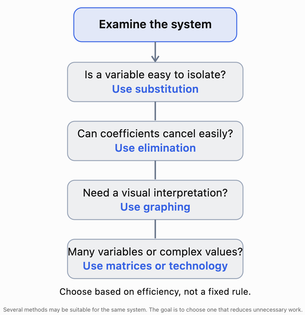
Worked Example: Comparing Substitution and Elimination
Solve:
3x + 2y = 18
x + y = 7
Method 1: Substitution
From the second equation:
y = 7 − x
Substitute into the first:
3x + 2(7 − x) = 18
3x + 14 − 2x = 18
x = 4
Then:
y = 7 − 4 = 3
Solution: (4, 3)
Method 2: Elimination
Multiply the second equation by 2:
2x + 2y = 14
Subtract from the first:
x = 4
Then:
4 + y = 7
y = 3
Solution: (4, 3)
Which method is more efficient?
Both methods require only a few steps.
Elimination avoids expanding brackets, while substitution uses the easily isolated variable.
Either is a reasonable choice.
Verification
3(4) + 2(3) = 18
4 + 3 = 7
Both equations are satisfied.
Important principle: Efficiency is not always about using the fewest written lines. A method that is easier to understand and less likely to produce errors may be the better choice.
Worked Example: Elimination with Different Coefficients
Solve:
3x + 4y = 25
5x − 2y = 7
Step 1: Identify the variable to eliminate
The y-coefficients are 4 and −2.
Multiplying the second equation by 2 creates opposite coefficients.
10x − 4y = 14
Step 2: Add the equations
3x + 4y = 25
10x − 4y = 14
Add:
13x = 39
x = 3
Step 3: Find y
Substitute into:
5x − 2y = 7
5(3) − 2y = 7
15 − 2y = 7
−2y = −8
y = 4
Step 4: Verify
3(3) + 4(4) = 9 + 16 = 25
5(3) − 2(4) = 15 − 8 = 7
Answer: (3, 4)
Why elimination is efficient
Only one equation needs to be multiplied.
The y-terms then cancel immediately, producing a simple equation in x.
Worked Example: A System Containing Fractions
Solve:
x/2 + y/3 = 5
x/4 − y/6 = 1
Step 1: Eliminate fractions
The least common multiple of 2 and 3 is 6.
Multiply the first equation by 6:
3x + 2y = 30
The least common multiple of 4 and 6 is 12.
Multiply the second equation by 12:
3x − 2y = 12
Step 2: Add
6x = 42
x = 7
Step 3: Find y
3(7) + 2y = 30
21 + 2y = 30
2y = 9
y = 9/2 = 4.5
Step 4: Verify
First equation:
7/2 + 4.5/3 = 3.5 + 1.5 = 5
Second equation:
7/4 − 4.5/6 = 1.75 − 0.75 = 1
Answer: x = 7, y = 4.5
Strategy lesson
When a system contains fractions, multiplying each equation by its least common denominator can simplify the calculations significantly.
Recognising the Number of Solutions
A system does not always have exactly one solution.
Unique solution
Consider:
x + y = 8
x − y = 2
Adding:
2x = 10
x = 5
y = 3
The system has one solution.
No solution
Consider:
2x + 4y = 12
x + 2y = 9
Multiplying the second equation by 2 gives:
2x + 4y = 18
But the first equation requires:
2x + 4y = 12
The equations contradict one another.
Conclusion: No solution.
Infinitely many solutions
Consider:
2x + 4y = 12
x + 2y = 6
Multiplying the second equation by 2 produces the first equation.
The equations represent the same line.
Conclusion: Infinitely many solutions.
Geometric interpretation
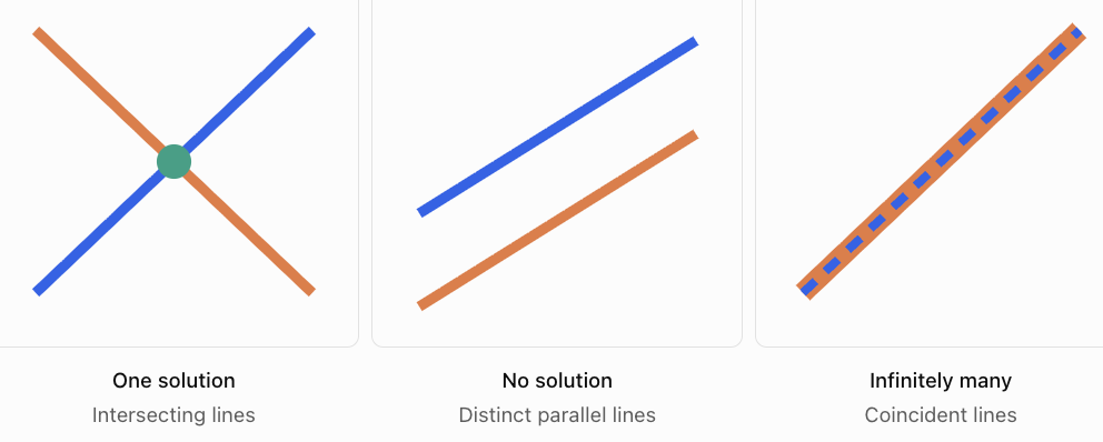
Integrated Problem: Three-Variable Systems
Some problems involve three unknown quantities and require several stages of elimination.
Solve:
x + y + z = 12
2x + 3y + z = 23
3x + y + 2z = 21
Step 1: Eliminate z
Subtract the first equation from the second:
x + 2y = 11
Multiply the first equation by 2:
2x + 2y + 2z = 24
Subtract this from the third equation:
x − y = −3
The reduced system is:
x + 2y = 11
x − y = −3
Step 2: Solve the reduced system
Subtract the second equation from the first:
3y = 14
y = 14/3
Substitute:
x − 14/3 = −3
x = 5/3
Step 3: Find z
x + y + z = 12
5/3 + 14/3 + z = 12
19/3 + z = 36/3
z = 17/3
Step 4: Verify
First equation:
5/3 + 14/3 + 17/3 = 36/3 = 12
Second equation:
2(5/3) + 3(14/3) + 17/3
= 10/3 + 14 + 17/3
= 27/3 + 14 = 23
Third equation:
3(5/3) + 14/3 + 2(17/3)
= 5 + 48/3 = 21
Answer: x = 5/3, y = 14/3, z = 17/3.
Strategy lesson
Three-variable systems can often be reduced to two-variable systems.
The most important step is eliminating the same variable from two different pairs of equations.
Integrated Problem: Nonlinear Systems
Solve:
x² + y² = 25
y = x + 1
This system contains a circle and a straight line.
Step 1: Choose a method
Substitution is appropriate because y is already isolated.
Step 2: Substitute
x² + (x + 1)² = 25
Expand:
x² + x² + 2x + 1 = 25
2x² + 2x − 24 = 0
Divide by 2:
x² + x − 12 = 0
Step 3: Factor
(x + 4)(x − 3) = 0
Therefore:
x = −4 or x = 3
Step 4: Find y-values
If x = −4:
y = −3
If x = 3:
y = 4
Step 5: Verify
For (−4, −3):
16 + 9 = 25
−3 = −4 + 1
For (3, 4):
9 + 16 = 25
4 = 3 + 1
Answers: (−4, −3) and (3, 4).
Interpretation
The line intersects the circle at two points.
Both solutions are necessary because the original problem asks for all intersections.
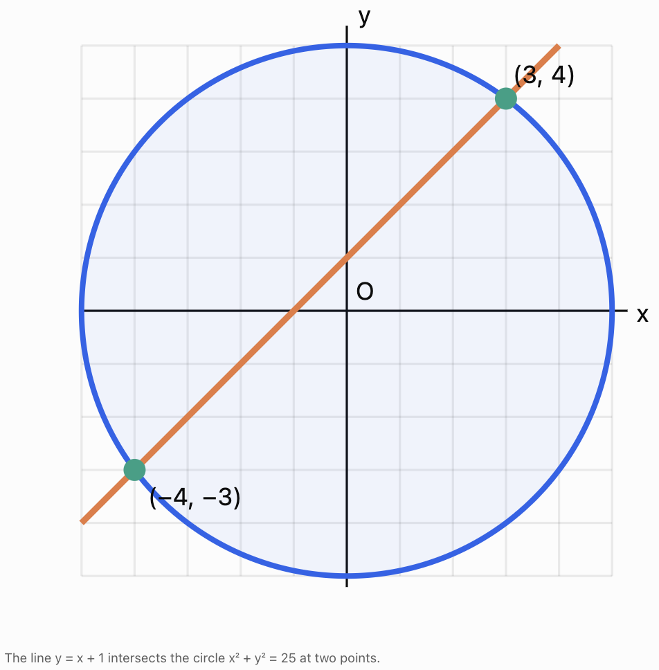
Integrated Problem: Business and Economics
A company manufactures two products, A and B.
Each unit of Product A requires 3 hours of labour and 2 kg of material.
Each unit of Product B requires 2 hours of labour and 4 kg of material.
The company uses 160 labour-hours and 160 kg of material.
Determine the number of units manufactured.
Step 1: Define variables
x = number of units of Product A
y = number of units of Product B
Step 2: Construct equations
Labour:
3x + 2y = 160
Materials:
2x + 4y = 160
Step 3: Select a method
Elimination is efficient because the second equation can be divided by 2.
x + 2y = 80
Subtract this from the labour equation:
2x = 80
x = 40
Step 4: Find y
40 + 2y = 80
2y = 40
y = 20
Step 5: Verify
Labour:
3(40) + 2(20) = 160 hours
Materials:
2(40) + 4(20) = 160 kg
Answer: 40 units of Product A and 20 units of Product B.
Evaluate the model
The result is reasonable because both quantities are nonnegative whole numbers.
However, the model assumes constant resource requirements, no waste, and that all recorded resources were used to manufacture these products.
Integrated Problem: Geometry and Algebra
A rectangular garden has a perimeter of 50 m and an area of 150 m².
Find its dimensions.
Step 1: Define variables
l = length, in metres
w = width, in metres
Step 2: Construct equations
Perimeter:
2l + 2w = 50
l + w = 25
Area:
lw = 150
Step 3: Choose a method
Substitution is appropriate because the perimeter equation can easily be rearranged.
l = 25 − w
Step 4: Substitute
(25 − w)w = 150
25w − w² = 150
w² − 25w + 150 = 0
Factor:
(w − 10)(w − 15) = 0
w = 10 or w = 15
The two values represent the same rectangle with the dimensions interchanged.
Answer: The garden measures 15 m by 10 m.
Step 5: Verify
Perimeter:
2(15) + 2(10) = 50 m
Area:
15(10) = 150 m²
Why this problem is important
It requires recognising that one geometric relationship is linear and another is nonlinear.
The problem cannot be solved using ordinary linear elimination alone without additional algebraic manipulation.
Integrated Problem: Science and Experimental Data
A scientist models the position of an object using:
s = vt + s₀
where:
-
s = position, in metres.
-
v = constant velocity, in m/s.
-
t = time, in seconds.
-
s₀ = initial position, in metres.
Measurements show:
|
Time (s) |
Position (m) |
|---|---|
|
2 |
11 |
|
6 |
27 |
Determine the velocity and initial position.
Step 1: Construct the equations
11 = 2v + s₀
27 = 6v + s₀
Step 2: Select a method
Elimination is efficient because both equations contain the same coefficient for s₀.
Subtract:
16 = 4v
v = 4 m/s
Step 3: Find initial position
11 = 2(4) + s₀
s₀ = 3 m
Step 4: Write the model
s = 4t + 3
Step 5: Verify
At t = 2 s:
s = 4(2) + 3 = 11 m
At t = 6 s:
s = 4(6) + 3 = 27 m
Answer: Velocity = 4 m/s and initial position = 3 m.
Evaluate
The model assumes constant velocity.
Two measurements determine the parameters of a linear model, but additional measurements are needed to test whether the motion is actually uniform.
Integrated Problem: An Unfamiliar Situation
A wildlife researcher counts two species of animals in a habitat.
Species A has 4 legs per animal.
Species B has 2 legs per animal.
There are 75 animals and 220 legs in total.
Find the number of animals of each species.
Step 1: Understand the situation
The problem does not initially provide algebraic equations.
We must identify the unknown quantities and translate the information into a mathematical model.
Step 2: Define variables
x = number of Species A animals
y = number of Species B animals
Step 3: Construct equations
Total animals:
x + y = 75
Total legs:
4x + 2y = 220
Step 4: Solve
Multiply the first equation by 2:
2x + 2y = 150
Subtract:
2x = 70
x = 35
Then:
y = 75 − 35
y = 40
Step 5: Verify
Total animals:
35 + 40 = 75
Total legs:
4(35) + 2(40)
= 140 + 80
= 220
Answer: 35 animals of Species A and 40 animals of Species B.
Step 6: Evaluate
The model assumes that the habitat contains only these two species and that every animal has the expected number of legs.
In an actual field investigation, sampling error or incomplete observations may affect the results.
General lesson
Unfamiliar problems become easier when we focus on identifying quantities and relationships rather than trying to memorise a particular question type.
Justifying Mathematical Reasoning
A mathematical justification explains why a particular step or method is valid.
Compare these two solutions.
Incomplete explanation
x = 5
y = 3
Complete explanation
The system is:
x + y = 8
x − y = 2
Elimination is efficient because the y-coefficients are opposites.
Adding the equations eliminates y:
2x = 10
Therefore:
x = 5
Substituting into x + y = 8:
y = 3
Checking:
5 + 3 = 8
5 − 3 = 2
Both equations are satisfied, so the solution is (5, 3).
The complete explanation identifies the method, justifies its selection, shows the calculations, and verifies the result.
What makes a strong justification?
A strong mathematical explanation should demonstrate:
-
Why the equations represent the problem.
-
Why the chosen method is suitable.
-
Why each algebraic transformation is valid.
-
How the solution satisfies the original conditions.
-
What the answer means in context.
Communicating Organised Solutions
A useful structure for written solutions is:
Understand → Define → Model → Solve → Verify → Interpret
Understand
Identify the known information and what must be determined.
Define
Introduce variables with clear meanings and units.
Model
Write the equations representing the relationships.
Solve
Choose an efficient method and show the algebraic steps.
Verify
Substitute the values into the original equations.
Interpret
Explain the answer in the original context.
For real-world problems, add an evaluation of the assumptions and limitations.
This structure makes solutions easier to follow, check, and communicate.
Common Errors in Integrated Problems
Error 1: Choosing an unnecessarily complicated method
Consider:
y = 2x + 3
x + y = 18
Using elimination without rearranging is possible, but substitution is more direct because y is already isolated.
Error 2: Incorrect distribution
Incorrect:
3(x + 2) = 3x + 2
Correct:
3(x + 2) = 3x + 6
Error 3: Changing only one term when multiplying an equation
Incorrect:
2x + y = 10
Multiply by 3:
6x + y = 30
Correct:
6x + 3y = 30
Every term must be multiplied.
Error 4: Losing a negative sign
Incorrect:
−2y = 8
y = 4
Correct:
y = −4
Error 5: Ignoring a second solution
A quadratic equation may produce two valid solutions.
For example:
x² = 16
x = −4 or x = 4
Both must be considered unless the original problem imposes restrictions.
Error 6: Confusing no solution with infinitely many solutions
A contradiction such as:
0 = 5
means no solution.
An identity such as:
0 = 0
means that the eliminated equation provides no additional restriction. In a two-variable linear system where both equations are equivalent, this leads to infinitely many solutions.
Error 7: Failing to interpret units
If x represents time in hours, the answer x = 4 should be communicated as 4 hours.
Error 8: Accepting an unrealistic result
A mathematical solution may be incompatible with the context.
Negative dimensions or fractional counts of complete objects should be investigated rather than automatically accepted.
Strategies for Unfamiliar Problems
When a problem appears unfamiliar, use the following reasoning process.
Identify quantities rather than keywords. Determine what is known and unknown.
Look for conservation relationships. Totals involving mass, cost, distance, or quantity often provide equations.
Look for comparisons. Statements such as “twice as many,” “five greater,” or “20% less” can be translated into equations.
Use a table when appropriate. Organising information often makes the relationships clearer.
Check the number of independent relationships. A unique solution generally requires enough independent information to determine the unknowns.
Choose a method based on the equation structure. Do not automatically use the same method for every problem.
Verify before interpreting. An algebraic error can lead to an incorrect real-world conclusion.
Evaluate the answer. Ask whether the values make sense and satisfy any practical restrictions.
Key Terms
-
System of equations: Two or more equations solved simultaneously.
-
Simultaneous solution: Values satisfying every equation in a system.
-
Substitution: Replacing a variable with an equivalent expression.
-
Elimination: Combining equations to remove a variable.
-
Graphical method: Solving or representing a system using graphs.
-
Matrix method: Representing and solving a system using matrices.
-
Linear system: A system consisting of linear equations.
-
Nonlinear system: A system containing at least one nonlinear equation.
-
Unique solution: Exactly one solution satisfying the system.
-
Inconsistent system: A system with no solution.
-
Dependent equations: Equations that do not provide independent information.
-
Equivalent equations: Equations having exactly the same solution set.
-
Mathematical model: A mathematical representation of a real-world situation.
-
Constraint: A restriction on possible solutions.
-
Verification: Checking whether a solution satisfies the original equations.
-
Interpretation: Explaining the mathematical result in context.
-
Justification: Explaining why a mathematical method or step is valid.
-
Efficiency: Solving a problem with a suitable balance of simplicity, accuracy, and clarity.
-
Extraneous solution: A candidate solution that does not satisfy the original problem.
-
Independent information: Information that contributes a new mathematical restriction.
Key Takeaways
-
Different systems may be best solved using different methods.
-
Substitution is often efficient when a variable is isolated.
-
Elimination is often efficient when coefficients can cancel.
-
Graphing provides a visual interpretation of solutions.
-
Matrix methods and technology are useful for larger systems.
-
Three-variable systems can often be reduced to two-variable systems.
-
Nonlinear systems may produce multiple solutions.
-
Some systems have no solution or infinitely many solutions.
-
Real-world problems require variables, equations, constraints, and interpretation.
-
Mathematical reasoning should be justified and clearly communicated.
-
Every solution should be checked against the original equations.
-
Unfamiliar problems can be approached systematically by identifying quantities and relationships.
Check Your Understanding
For each problem, select an efficient method, show your working, and verify your solution. For application questions, explain what your answer means in context.
Part A: Selecting Methods
1. Identify the most efficient method for solving each system and explain your choice.
a) y = 4x − 3 and x + y = 17
b) 3x + 2y = 16 and 5x − 2y = 8
c) y = x² − 4 and y = 2x − 4
d) x + y + z = 12, 2x − y + z = 9, and x + 2y − z = 3
2. Explain why elimination is usually efficient when two equations contain opposite coefficients for one variable.
3. Explain why graphing may not always provide an exact solution.
Part B: Algebraic Systems
4. Solve:
2x + 3y = 19
4x − 3y = 5
5. Solve:
y = 3x − 2
2x + y = 18
6. Solve:
x/2 + y/4 = 5
x/3 − y/6 = 1
7. Determine whether the following system has one solution, no solution, or infinitely many solutions:
3x + 6y = 18
x + 2y = 6
8. Determine the number of solutions:
2x − 4y = 10
x − 2y = 8
Part C: Advanced Systems
9. Solve:
x + y + z = 10
2x − y + z = 9
x + 2y − z = 3
10. Find all intersection points of:
x² + y² = 25
y = x + 1
11. Solve:
xy = 24
x + y = 10
Part D: Integrated Applications
12. A school sells adult tickets for $18 and student tickets for $12.
A total of 150 tickets are sold, generating $2,250.
Determine the number of each ticket type.
13. A rectangle has a perimeter of 46 cm and an area of 120 cm².
Find its dimensions.
14. Two vehicles travel in opposite directions from the same starting point.
After 3 hours, they are 270 km apart.
One vehicle travels 10 km/h faster than the other.
Find their speeds.
15. A laboratory needs 400 mL of a 30% solution.
It has a 20% solution and a 50% solution.
Assuming compatible concentrations and additive volumes, determine how much of each is required.
16. A company manufactures two products.
Product A requires 4 labour-hours and 3 units of material.
Product B requires 2 labour-hours and 5 units of material.
The company uses 100 labour-hours and 110 units of material.
Determine the production quantities and evaluate whether the result is realistic.
Part E: Analysis and Mathematical Reasoning
17. A student solves:
2x + y = 12
x − y = 3
and obtains x = 3, y = 6.
Identify the error by checking the solution, then find the correct answer.
18. A system produces the solution:
x = −5
y = 12
Explain why this may be acceptable in coordinate geometry but unacceptable in a problem involving physical dimensions.
19. A scientist constructs a two-variable model using two experimental measurements. The model has a unique solution, but a third measurement does not agree with its predictions.
Explain what the scientist should investigate.
20. Integrated Challenge
A school sells three types of merchandise:
-
Pens for $2 each.
-
Notebooks for $5 each.
-
T-shirts for $12 each.
A total of 100 items are sold for $500.
The number of pens sold is twice the number of T-shirts.
Determine the number of each item, verify your answer, and explain why a three-variable system is appropriate.
Answers to Check Your Understanding
1. Selecting methods
a) Substitution. The first equation already isolates y.
b) Elimination. The y-coefficients are +2 and −2, so they cancel immediately.
c) Substitution. Both equations express y in terms of x, allowing the expressions to be set equal.
d) Elimination or matrices. Three unknowns require combining equations systematically.
2. Why opposite coefficients help
When the equations are added, the terms with opposite coefficients cancel, leaving an equation with fewer unknowns.
This reduces the amount of algebra required.
3. Graphing limitations
A graph may show only approximate intersection coordinates.
The graphing window, display resolution, and scale can also affect accuracy.
Algebraic methods are often preferable when exact values are required.
4. Elimination
2x + 3y = 19
4x − 3y = 5
Add:
6x = 24
x = 4
Substitute:
2(4) + 3y = 19
3y = 11
y = 11/3
Answer: (4, 11/3).
Verification:
2(4) + 3(11/3) = 19
4(4) − 3(11/3) = 5
5. Substitution
y = 3x − 2
2x + y = 18
Substitute:
2x + 3x − 2 = 18
5x = 20
x = 4
y = 3(4) − 2 = 10
Answer: (4, 10).
6. Fractions
x/2 + y/4 = 5
Multiply by 4:
2x + y = 20
x/3 − y/6 = 1
Multiply by 6:
2x − y = 6
Add:
4x = 26
x = 13/2
Then:
y = 20 − 2(13/2)
y = 7
Answer: x = 13/2, y = 7.
Verification:
(13/2)/2 + 7/4 = 13/4 + 7/4 = 5
(13/2)/3 − 7/6 = 13/6 − 7/6 = 1
7. Infinitely many solutions
3x + 6y = 18
x + 2y = 6
Multiplying the second equation by 3 produces the first.
Answer: Infinitely many solutions.
The equations represent the same line.
8. No solution
2x − 4y = 10
x − 2y = 8
Multiply the second equation by 2:
2x − 4y = 16
The same expression cannot equal both 10 and 16.
Answer: No solution.
9. Three-variable system
x + y + z = 10
2x − y + z = 9
x + 2y − z = 3
Subtract the first equation from the second:
x − 2y = −1
Add the first and third equations:
2x + 3y = 13
From the first reduced equation:
x = 2y − 1
Substitute:
2(2y − 1) + 3y = 13
7y − 2 = 13
7y = 15
y = 15/7
Then:
x = 2(15/7) − 1 = 23/7
Using the first original equation:
z = 10 − 23/7 − 15/7
z = 32/7
Answer: x = 23/7, y = 15/7, z = 32/7.
Verification:
First equation: (23 + 15 + 32)/7 = 10
Second equation: (46 − 15 + 32)/7 = 9
Third equation: (23 + 30 − 32)/7 = 3
10. Line-circle intersections
Substitute y = x + 1:
x² + (x + 1)² = 25
2x² + 2x − 24 = 0
x² + x − 12 = 0
(x + 4)(x − 3) = 0
x = −4 or x = 3
Corresponding y-values:
y = −3 or y = 4
Answer: (−4, −3) and (3, 4).
11. Product and sum
xy = 24
x + y = 10
Rearrange:
y = 10 − x
Substitute:
x(10 − x) = 24
10x − x² = 24
x² − 10x + 24 = 0
(x − 4)(x − 6) = 0
x = 4 or x = 6
Answers: (4, 6) and (6, 4).
Both satisfy the original system.
12. Ticket sales
Let:
a = adult tickets
s = student tickets
a + s = 150
18a + 12s = 2250
Multiply the first equation by 12:
12a + 12s = 1800
Subtract:
6a = 450
a = 75
Then:
s = 75
Answer: 75 adult tickets and 75 student tickets.
Verification:
18(75) + 12(75) = $2250
13. Rectangle dimensions
Let:
l = length
w = width
Perimeter:
l + w = 23
Area:
lw = 120
Substitute l = 23 − w:
(23 − w)w = 120
w² − 23w + 120 = 0
(w − 8)(w − 15) = 0
Answer: 15 cm by 8 cm.
Verification:
2(15) + 2(8) = 46 cm
15(8) = 120 cm²
14. Vehicle speeds
Let:
x = slower speed
y = faster speed
3x + 3y = 270
x + y = 90
y − x = 10
Add:
2y = 100
y = 50
x = 40
Answer: 40 km/h and 50 km/h.
Verification:
3(40) + 3(50) = 270 km
15. Solution mixture
Let:
x = volume of 20% solution
y = volume of 50% solution
x + y = 400
0.20x + 0.50y = 120
Substitute x = 400 − y:
80 − 0.20y + 0.50y = 120
0.30y = 40
y = 400/3 ≈ 133.33 mL
Then:
x = 800/3 ≈ 266.67 mL
Answer: Approximately 266.67 mL of 20% solution and 133.33 mL of 50% solution.
Use the exact fractional values for verification to avoid rounding error.
16. Manufacturing
Let:
x = Product A units
y = Product B units
Labour:
4x + 2y = 100
Materials:
3x + 5y = 110
Divide the labour equation by 2:
2x + y = 50
Therefore:
y = 50 − 2x
Substitute:
3x + 5(50 − 2x) = 110
3x + 250 − 10x = 110
−7x = −140
x = 20
Then:
y = 10
Answer: 20 units of Product A and 10 units of Product B.
Verification:
4(20) + 2(10) = 100 hours
3(20) + 5(10) = 110 units of material
The quantities are nonnegative whole numbers, so they are feasible under the stated assumptions.
17. Error analysis
The student's proposed solution is:
x = 3, y = 6
Check the first equation:
2(3) + 6 = 12
This is correct.
Check the second equation:
3 − 6 = −3
But the equation requires +3.
Therefore, the proposed values do not solve the system.
To correct the solution:
2x + y = 12
x − y = 3
Add:
3x = 15
x = 5
Then:
5 − y = 3
y = 2
Correct answer: (5, 2).
Both equations are satisfied.
18. Negative solutions
Negative coordinates are valid in coordinate geometry.
For example, x = −5 may represent a point 5 units to the left of the y-axis.
However, a negative physical length or width is not meaningful in ordinary geometric measurement.
The context determines whether a negative value is acceptable.
19. Model evaluation
The scientist should investigate whether the model's assumptions are appropriate.
Possible issues include measurement uncertainty, incorrect data, changing experimental conditions, or a relationship that is not truly linear.
Additional measurements and a revised model may be necessary.
20. Integrated challenge
Let:
p = number of pens
n = number of notebooks
t = number of T-shirts
Total items:
p + n + t = 100
Revenue:
2p + 5n + 12t = 500
Quantity relationship:
p = 2t
Substitute into the first equation:
2t + n + t = 100
n = 100 − 3t
Substitute into the revenue equation:
2(2t) + 5(100 − 3t) + 12t = 500
4t + 500 − 15t + 12t = 500
t = 0
Then:
p = 0
n = 100
Answer: 0 pens, 100 notebooks, and 0 T-shirts.
Verification:
Total items:
0 + 100 + 0 = 100
Revenue:
2(0) + 5(100) + 12(0) = $500
Quantity relationship:
0 = 2(0)
All conditions are satisfied.
The system requires three variables because the school sells three different types of merchandise.
The result is mathematically valid, although it is a boundary case in which only notebooks were sold. If the problem required at least one of every item, the information would be inconsistent with that additional requirement.
Final Summary
Solving systems of equations confidently requires more than memorising algebraic procedures.
It involves recognising mathematical structures, choosing efficient methods, constructing models, justifying calculations, and interpreting solutions.
The strongest problem-solvers are flexible. They can use substitution when a variable is isolated, elimination when coefficients can cancel, graphing when visual interpretation is useful, and technology when systems become more complex.
They also recognise when a system has no solution, infinitely many solutions, or multiple solutions arising from nonlinear relationships.
Most importantly, they verify their calculations and communicate their conclusions clearly.
Successful integrated problem-solving means choosing an appropriate strategy, applying it accurately, explaining why it works, and determining whether the result makes sense.