Applications and Mathematical Modelling

Introduction

Science uses mathematics to describe, explain, and predict how the natural world behaves. Whether scientists are studying the motion of objects, analysing chemical reactions, measuring electrical circuits, or investigating experimental data, they frequently encounter situations involving several unknown quantities.

A system of equations allows scientists to combine different pieces of information and determine unknown values.

For example, a scientist might need to determine:

• The masses of two substances in a mixture.

• The speeds of two moving objects.

• The forces acting on an object in equilibrium.

• The currents flowing through different parts of an electrical circuit.

• The concentrations of solutions prepared in a laboratory.

• The unknown parameters in an experimental model.

Each measurement or scientific law provides a mathematical relationship. When enough independent relationships are available, the unknown quantities can often be determined.

Systems of equations are especially useful because they allow scientists to analyse several connected quantities simultaneously.

However, scientific models are simplified representations of reality. A mathematically correct solution must still be evaluated using scientific principles, appropriate units, experimental uncertainty, and the assumptions of the model.

Why Are Systems of Equations Important in Science?

Scientific investigations often involve multiple unknown quantities.

Consider a laboratory mixture containing two liquids.

A scientist knows:

• The total volume of the mixture.

• The total mass of the mixture.

• The densities of the two liquids.

The scientist wants to determine the volume of each liquid.

One equation can describe the total volume.

Another equation can describe the total mass.

Together, these equations form a system that can determine both unknown volumes.

This approach is used across many scientific disciplines.

The general process is similar in every field:

Scientific information → Mathematical equations → Solution → Scientific interpretation → Verification

Building a Mathematical Model from Scientific Information

A mathematical model represents a scientific situation using variables and equations.

A reliable modelling process involves several steps.

Step 1: Identify the unknown quantities

Define variables clearly and include their units.

For example:

m₁ = mass of substance A, in grams

m₂ = mass of substance B, in grams

Step 2: Identify the scientific relationships

Look for relevant scientific laws or definitions.

Examples include:

Speed = distance/time

Density = mass/volume

Force = mass × acceleration

Charge = current × time

Concentration = mass of solute/volume of solution

Step 3: Construct equations

Use the information in the problem to create relationships between the variables.

Step 4: Solve the system

Choose an appropriate method:

• Substitution.

• Elimination.

• Graphing.

• Matrix methods.

• Technology.

Step 5: Interpret the solution

Explain what each value represents and include correct units.

Step 6: Verify the result

Substitute the values into the original equations and check whether they satisfy the scientific conditions.

Step 7: Evaluate the model

Consider whether the assumptions are realistic and whether the measurements are sufficiently accurate.

Application: Mixing Two Liquids Using Density

Density describes how much mass is contained in a given volume.

The density equation is:

ρ = m/V

where:

• ρ = density.

• m = mass.

• V = volume.

Rearranging:

m = ρV

Suppose a laboratory technician mixes two liquids.

Liquid A has a density of 0.8 g/mL.

Liquid B has a density of 1.2 g/mL.

The mixture has:

• Total volume = 100 mL.

• Total mass = 104 g.

Assuming the volumes are additive, determine the volume of each liquid.

Step 1: Define variables

x = volume of Liquid A, in mL

y = volume of Liquid B, in mL

Step 2: Construct the volume equation

The total volume is 100 mL.

x + y = 100

Step 3: Construct the mass equation

Mass = density × volume

Liquid A has mass:

0.8x

Liquid B has mass:

1.2y

The total mass is 104 g.

0.8x + 1.2y = 104

Step 4: Solve by substitution

From the volume equation:

x = 100 − y

Substitute:

0.8(100 − y) + 1.2y = 104

80 − 0.8y + 1.2y = 104

0.4y = 24

y = 60

Then:

x = 100 − 60

x = 40

Step 5: Interpret

Liquid A: 40 mL

Liquid B: 60 mL

Step 6: Verify

Total volume:

40 + 60 = 100 mL

Total mass:

0.8(40) + 1.2(60)

= 32 + 72

= 104 g

Both conditions are satisfied.

Answer: The mixture contains 40 mL of Liquid A and 60 mL of Liquid B.

Limitations of the model

The calculation assumes that the volumes are additive.

In real mixtures, molecular interactions can cause the final volume to differ from the sum of the separate volumes.

The model also assumes that the densities remain constant at the experimental temperature.

These assumptions must be considered before applying the result to an actual laboratory mixture.

Application: Preparing Solutions of Different Concentrations

Scientists often prepare solutions by combining liquids with different concentrations.

Suppose a laboratory needs 500 mL of a 20% solution.

Two solutions are available:

• Solution A: 10%.

• Solution B: 30%.

How much of each solution is required?

Step 1: Define variables

x = volume of 10% solution, in mL

y = volume of 30% solution, in mL

Step 2: Total volume equation

x + y = 500

Step 3: Solute equation

The amount of solute in each solution is proportional to its concentration.

0.10x + 0.30y = 0.20(500)

Therefore:

0.10x + 0.30y = 100

The equation uses equivalent volumes of solute under a simplified volume-percent model.

Step 4: Solve

From the first equation:

x = 500 − y

Substitute:

0.10(500 − y) + 0.30y = 100

50 − 0.10y + 0.30y = 100

0.20y = 50

y = 250

Then:

x = 500 − 250

x = 250

Step 5: Interpret

250 mL of the 10% solution

250 mL of the 30% solution

Step 6: Verify

Total volume:

250 + 250 = 500 mL

Solute-equivalent volume:

0.10(250) + 0.30(250)

= 25 + 75

= 100 mL

Final concentration:

100/500 × 100% = 20%

Answer: Mix 250 mL of each solution.

Scientific interpretation

The required concentration lies halfway between 10% and 30%.

Therefore, equal volumes produce the desired 20% concentration under the model's assumptions.

Important limitation

This simplified model assumes consistent concentration definitions and additive volumes. In laboratory work, concentration units such as mol/L, g/L, and mass percent must not be mixed without conversion.

For precise solution preparation, a laboratory may need to measure solute quantity and dilute to a specified final volume rather than simply add two measured volumes.

Application: Motion of Two Objects

Systems of equations can be used to analyse objects moving at constant speeds.

The basic relationship is:

d = vt

where:

• d = distance.

• v = speed.

• t = time.

Worked Example: Two Cyclists

Two cyclists begin travelling from the same location in opposite directions.

After 3 hours, they are 90 km apart.

One cyclist travels 6 km/h faster than the other.

Find their speeds.

Step 1: Define variables

x = speed of the slower cyclist, in km/h

y = speed of the faster cyclist, in km/h

Step 2: Construct the distance equation

The slower cyclist travels:

3x kilometres

The faster cyclist travels:

3y kilometres

Since they travel in opposite directions, their separation is the sum of the distances.

3x + 3y = 90

Divide by 3:

x + y = 30

Step 3: Construct the speed equation

The faster cyclist travels 6 km/h faster.

y − x = 6

Step 4: Solve

Add the equations:

x + y = 30

−x + y = 6

2y = 36

y = 18

Then:

x = 30 − 18

x = 12

Step 5: Verify

Slower cyclist:

d = 12(3) = 36 km

Faster cyclist:

d = 18(3) = 54 km

Total separation:

36 + 54 = 90 km

Speed difference:

18 − 12 = 6 km/h

Answer: The slower cyclist travels at 12 km/h, and the faster cyclist travels at 18 km/h.

Limitations of the model

The calculation assumes that both cyclists:

• Travel in exactly opposite directions along the same straight route.

• Maintain constant speeds.

• Start at the same time.

• Do not stop during the journey.

Real journeys may involve acceleration, changes in direction, and stops.

The model is therefore an approximation of actual motion.

Application: Forces in Equilibrium

An object is in equilibrium when the resultant force acting on it is zero.

For equilibrium in two dimensions:

ΣFₓ = 0

ΣFᵧ = 0

These equations can be used together to determine unknown forces.

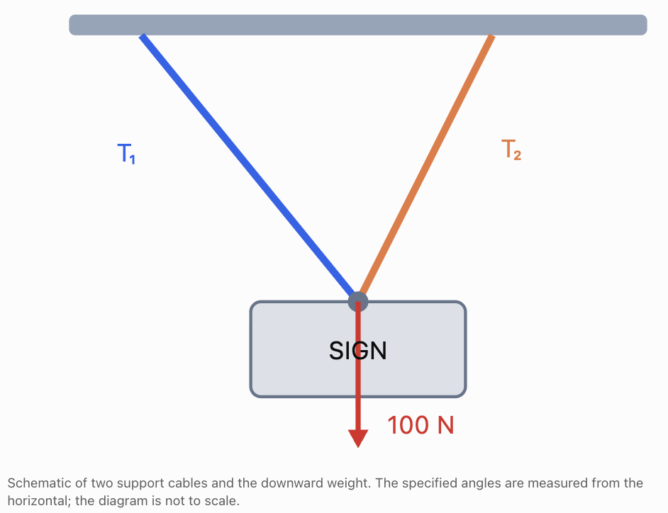
Worked Example: A Hanging Sign

A sign weighing 100 N is supported by two cables.

The left cable makes an angle of 30° above the horizontal.

The right cable makes an angle of 60° above the horizontal.

Determine the tension in each cable.

Step 1: Define variables

T₁ = tension in the left cable, in N

T₂ = tension in the right cable, in N

Step 2: Resolve the forces horizontally

The horizontal components must balance.

The left cable pulls left.

The right cable pulls right.

T₁ cos 30° = T₂ cos 60°

Using:

cos 30° ≈ 0.866

cos 60° = 0.5

We obtain:

0.866T₁ = 0.5T₂

Therefore:

T₂ ≈ 1.732T₁

Step 3: Resolve the forces vertically

The upward components must balance the 100 N weight.

T₁ sin 30° + T₂ sin 60° = 100

Using:

sin 30° = 0.5

sin 60° ≈ 0.866

We obtain:

0.5T₁ + 0.866T₂ = 100

Step 4: Substitute

0.5T₁ + 0.866(1.732T₁) ≈ 100

0.5T₁ + 1.5T₁ ≈ 100

2T₁ ≈ 100

T₁ ≈ 50 N

Then:

T₂ ≈ 1.732(50)

T₂ ≈ 86.6 N

Step 5: Interpret

Left cable tension ≈ 50 N

Right cable tension ≈ 86.6 N

The right cable has greater tension because its steeper angle changes how the force is distributed between horizontal and vertical components.

Step 6: Verify

Horizontal:

50 cos 30° ≈ 86.6 cos 60°

43.3 N ≈ 43.3 N

Vertical:

50 sin 30° + 86.6 sin 60°

≈ 25 + 75

≈ 100 N

Answer: T₁ = 50 N and T₂ ≈ 86.6 N.

Scientific assumptions

This model assumes:

• The sign is stationary.

• The cables are massless.

• The cable angles are known accurately.

• No additional horizontal forces act.

• The sign is treated as a particle at the support junction, or the support geometry also satisfies rotational equilibrium.

In real engineering problems, the sign's dimensions, attachment points, and torque balance may also need to be considered.

Application: Electrical Circuits

Electrical circuits can be analysed using systems of equations.

Two important principles are:

Kirchhoff's Current Law

The total current entering a junction equals the total current leaving the junction.

Kirchhoff's Voltage Law

The sum of voltage changes around a closed circuit loop equals zero.

Ohm's Law is also important:

V = IR

where:

• V = potential difference, in volts.

• I = current, in amperes.

• R = resistance, in ohms.

Worked Example: Currents in a Circuit

At a junction, a total current of 6 A splits into two branches.

The first branch has resistance 4 Ω.

The second branch has resistance 8 Ω.

Both branches are connected in parallel, so the potential difference across each branch is equal.

Find the current in each branch.

Step 1: Define variables

I₁ = current through the 4 Ω branch, in A

I₂ = current through the 8 Ω branch, in A

Step 2: Apply the current law

I₁ + I₂ = 6

Step 3: Apply Ohm's Law

The voltage across each branch is the same.

4I₁ = 8I₂

Divide by 4:

I₁ = 2I₂

Step 4: Solve

Substitute:

2I₂ + I₂ = 6

3I₂ = 6

I₂ = 2 A

Then:

I₁ = 4 A

Step 5: Verify

Total current:

4 + 2 = 6 A

Voltage across first branch:

V₁ = 4(4) = 16 V

Voltage across second branch:

V₂ = 8(2) = 16 V

Both branches have the same potential difference.

Answer: The 4 Ω branch carries 4 A, and the 8 Ω branch carries 2 A.

Scientific interpretation

The branch with lower resistance carries more current when the voltage is the same.

This agrees with Ohm's Law.

Model limitations

The calculation assumes ideal resistors with constant resistance.

In real circuits, resistance can change with temperature, and components may not behave ideally.

Application: Determining Unknown Quantities from Experimental Data

Scientific experiments often produce measurements that can be used to construct equations.

Consider a spring that follows Hooke's Law:

F = kx

where:

• F = applied force, in newtons.

• k = spring constant, in N/m.

• x = extension, in metres.

A real experimental setup may also contain a constant force offset caused by calibration error or another systematic effect.

A more general linear model is:

F = kx + b

where b represents the force offset.

Worked Example: Finding the Spring Constant

An experiment produces the following data:

Assume the relationship is linear.

Find k and b.

Step 1: Define variables

k = spring constant, in N/m

b = force offset, in N

Step 2: Construct equations

First measurement:

3 = 0.02k + b

Second measurement:

7 = 0.06k + b

Step 3: Eliminate b

Subtract:

7 − 3 = (0.06 − 0.02)k

4 = 0.04k

k = 100 N/m

Step 4: Find b

3 = 0.02(100) + b

3 = 2 + b

b = 1 N

Step 5: Write the model

F = 100x + 1

where F is in N and x is in m.

Step 6: Interpret

The gradient is 100 N/m.

This represents the spring constant in the linear model.

The intercept is 1 N.

This indicates that the measured force includes a constant offset.

Step 7: Verify

At x = 0.02 m:

F = 100(0.02) + 1 = 3 N

At x = 0.06 m:

F = 100(0.06) + 1 = 7 N

Both measurements are reproduced.

Limitations

Two data points always determine a straight line when their x-values are different.

However, this does not prove that the physical relationship is perfectly linear.

Scientists should collect additional measurements and examine whether the model remains appropriate.

The spring may also stop following Hooke's Law beyond its elastic limit.

Application: Determining a Linear Motion Model

A moving object has position described by:

s = vt + s₀

where:

• s = position, in metres.

• v = constant velocity, in m/s.

• t = time, in seconds.

• s₀ = initial position, in metres.

A motion sensor records:

At t = 2 s, s = 11 m.

At t = 5 s, s = 23 m.

Determine the velocity and initial position.

Step 1: Construct equations

11 = 2v + s₀

23 = 5v + s₀

Step 2: Eliminate s₀

Subtract:

12 = 3v

v = 4 m/s

Step 3: Find initial position

11 = 2(4) + s₀

s₀ = 3 m

Step 4: Write the motion model

s = 4t + 3

Step 5: Verify

At t = 2 s:

s = 4(2) + 3 = 11 m

At t = 5 s:

s = 4(5) + 3 = 23 m

Answer: Velocity = 4 m/s; initial position = 3 m.

Scientific interpretation

The object moves in the positive direction at a constant velocity of 4 m/s.

At t = 0, its position is 3 m.

Limitation

The model assumes constant velocity.

If the object accelerates, a linear position-time equation may no longer be appropriate.

Application: Biology and Population Studies

Systems of equations can be used to estimate populations when several measurements are available.

Worked Example: Two Species in a Habitat

An ecological survey identifies two species of animals in a protected habitat.

Species A has 4 legs per animal.

Species B has 2 legs per animal.

The survey records:

• 50 animals in total.

• 160 legs in total.

Determine the number of animals of each species.

Step 1: Define variables

x = number of four-legged animals

y = number of two-legged animals

Step 2: Construct equations

Total animals:

x + y = 50

Total legs:

4x + 2y = 160

Step 3: Solve

Multiply the first equation by 2:

2x + 2y = 100

Subtract from the second:

2x = 60

x = 30

Then:

y = 50 − 30

y = 20

Step 4: Verify

Total animals:

30 + 20 = 50

Total legs:

4(30) + 2(20)

= 120 + 40

= 160

Answer: There are 30 four-legged animals and 20 two-legged animals.

Scientific limitations

The model assumes:

• Only the two specified species are present.

• Every animal has the expected number of legs.

• All animals are counted correctly.

• The recorded observations are accurate.

In a real ecological investigation, incomplete observations and sampling errors may affect the results.

Application: Chemical Reactions and Conservation of Mass

Chemical reactions obey the law of conservation of mass.

In a closed system, the total mass of reactants equals the total mass of products.

Systems of equations can be used to determine unknown masses.

Worked Example: Formation of a Compound

Two elements, A and B, react to form a compound.

The total mass of the compound is 60 g.

The mass of element A is twice the mass of element B.

Find the mass of each element.

Step 1: Define variables

x = mass of element A, in g

y = mass of element B, in g

Step 2: Construct equations

Conservation of mass:

x + y = 60

Mass relationship:

x = 2y

Step 3: Solve

Substitute:

2y + y = 60

3y = 60

y = 20

Then:

x = 40

Step 4: Verify

40 + 20 = 60 g

40 = 2(20)

Answer: Element A contributes 40 g and element B contributes 20 g.

Scientific interpretation

The compound contains 40 g of element A and 20 g of element B.

The mass ratio is:

A : B = 2 : 1

This example assumes complete reaction, no loss of material, and that the compound contains only the two elements.

In actual chemistry, chemical formulae and mole ratios must also be considered when determining how elements combine.

Application: Three-Variable Scientific Systems

More complex scientific situations may involve three unknown quantities.

Worked Example: Three Materials in a Mixture

A laboratory combines three materials, A, B, and C.

Their densities are:

The total volume is 100 mL.

The total mass is 210 g.

The volume of Material C is 10 mL greater than the volume of Material A.

Determine the volume of each material.

Step 1: Define variables

x = volume of Material A, in mL

y = volume of Material B, in mL

z = volume of Material C, in mL

Step 2: Construct equations

Total volume:

x + y + z = 100

Total mass:

x + 2y + 3z = 210

Volume relationship:

z − x = 10

Step 3: Eliminate x

Subtract the total volume equation from the mass equation:

y + 2z = 110

Step 4: Use the third equation

z = x + 10

Therefore:

x = z − 10

Substitute into the volume equation:

(z − 10) + y + z = 100

y + 2z = 110

The reduced equations are identical.

Step 5: Interpret

The system does not have a unique solution.

The third relationship is already implied by the total mass and volume equations.

We can express the solutions using z = t:

x = t − 10

y = 110 − 2t

z = t

For nonnegative volumes:

10 ≤ t ≤ 55

There are infinitely many nonnegative real solutions.

Scientific conclusion

The available measurements are insufficient to determine the exact volume of each material.

An additional independent measurement is required.

For example, measuring the volume of one component would allow the remaining volumes to be determined.

Why this example matters

Scientific investigations do not always provide enough information to determine every unknown.

Recognising insufficient information is an important part of scientific reasoning.

Improving Experimental Models with Additional Measurements

Suppose the scientist measures the volume of Material B and finds:

y = 30 mL

Using:

y + 2z = 110

30 + 2z = 110

2z = 80

z = 40 mL

Then:

x = z − 10

x = 30 mL

The volumes are:

Material A: 30 mL

Material B: 30 mL

Material C: 40 mL

Verify

Total volume:

30 + 30 + 40 = 100 mL

Total mass:

1(30) + 2(30) + 3(40)

= 30 + 60 + 120

= 210 g

Volume difference:

40 − 30 = 10 mL

Answer: 30 mL of A, 30 mL of B, and 40 mL of C.

The additional independent measurement allows a unique solution to be determined.

Using Experimental Data to Construct Systems

Scientists frequently collect measurements and use them to determine unknown parameters.

Consider a relationship of the form:

y = mx + b

where:

m = gradient

b = y-intercept

Suppose an experiment produces:

The equations are:

7 = 2m + b

16 = 5m + b

Subtract:

9 = 3m

m = 3

Then:

7 = 2(3) + b

b = 1

The model is:

y = 3x + 1

Interpreting the parameters

The gradient represents the rate of change of y with respect to x.

The intercept represents the predicted value of y when x = 0.

The scientific meaning and units of these parameters depend on what x and y represent.

For example, if y is distance in metres and x is time in seconds:

m = 3 m/s

b = 1 m

The equation becomes:

s = 3t + 1

Why More Experimental Data Is Often Better

Two measurements can determine the gradient and intercept of a straight line.

However, real experimental measurements contain uncertainty.

For example:

These points are close to the relationship:

s = 3t + 1

But they do not lie exactly on one straight line.

This is common in experimental science.

Rather than constructing a system using only two measurements, scientists often use a line of best fit.

A best-fit line considers all available measurements and reduces the influence of random experimental variation.

Least-squares modelling

For a linear model:

y = mx + b

the least-squares method chooses m and b to minimise the sum of squared differences between measured and predicted values.

These differences are called residuals.

The resulting calculation can be expressed as a system of equations for m and b.

For n data points (xᵢ, yᵢ), the least-squares normal equations are:

mΣxᵢ² + bΣxᵢ = Σxᵢyᵢ

mΣxᵢ + nb = Σyᵢ

Solving this two-variable system gives the least-squares gradient and intercept, provided the x-values are not all identical.

This is an important connection between systems of equations and scientific data analysis.

At an introductory level, graphing software or spreadsheets can perform the calculation without requiring students to derive the equations.

Evaluating the Limitations of Mathematical Models

A mathematical model is useful only when its assumptions are appropriate for the situation being studied.

Scientific models simplify reality so that relationships can be represented mathematically.

However, simplification introduces limitations.

Limitation 1: Measurement Uncertainty

Scientific measurements are not perfectly exact.

For example, a measuring cylinder might record a volume of:

50.0 ± 0.5 mL

The actual volume may differ slightly from the recorded value.

When measured quantities are used in a system of equations, the calculated solution also contains uncertainty.

Limitation 2: Simplified Physical Conditions

A motion model may assume constant velocity.

A force model may ignore air resistance.

A circuit model may assume constant resistance.

A mixture model may assume additive volumes.

These assumptions can make the equations easier to solve but may reduce accuracy.

Limitation 3: Limited Experimental Data

A system may contain insufficient independent information.

For example:

x + y = 10

2x + 2y = 20

The second equation provides no new information.

The system has infinitely many solutions.

Additional independent measurements are needed to determine unique values.

Limitation 4: Inconsistent Data

Experimental measurements may contradict one another.

For example:

x + y = 10

x + y = 12

These equations cannot both be satisfied exactly.

This may indicate measurement error, an incorrect model, or incompatible experimental conditions.

Limitation 5: Sensitivity to Measurement Errors

Some systems are particularly sensitive to small changes in measured values.

Consider:

x + y = 10

x + 1.001y = 10.002

Subtract:

0.001y = 0.002

y = 2

Then:

x = 8

Now suppose the second measured constant changes slightly:

x + 1.001y = 10.003

Subtract:

0.001y = 0.003

y = 3

Then:

x = 7

A change of only 0.001 in one measured value changes the solution from (8, 2) to (7, 3).

This occurs because the equations represent lines with very similar slopes.

Such systems are described as ill-conditioned.

They can be difficult to solve accurately when experimental measurements contain uncertainty.

Limitation 6: Real-World Constraints

Scientific quantities may have restrictions.

Examples include:

• Mass cannot be negative.

• Volume cannot be negative.

• Population counts must be whole numbers.

• Concentration cannot exceed certain physical limits.

• A spring cannot stretch indefinitely while continuing to obey Hooke's Law.

A mathematical solution that violates these restrictions may be physically invalid.

Comparing Mathematical and Scientific Validity

A mathematically correct answer satisfies the equations.

A scientifically valid answer must also be consistent with physical laws, units, assumptions, and experimental conditions.

This distinction is essential when using mathematics in scientific investigations.

Communicating Scientific Conclusions

A strong scientific conclusion should do more than state a numerical answer.

It should include:

1. The calculated result.

2. Appropriate units.

3. An explanation of what the result means.

4. Verification using the original information.

5. Relevant assumptions or limitations.

Example: Basic conclusion

x = 40

y = 60

Improved scientific conclusion

The mixture contains 40 mL of Liquid A and 60 mL of Liquid B.

Strong scientific conclusion

The calculated mixture contains 40 mL of Liquid A and 60 mL of Liquid B. These volumes total 100 mL and produce a combined mass of 104 g using the given densities. The result is valid under the assumptions that the volumes are additive and the densities remain constant at the experimental temperature.

The final version demonstrates mathematical accuracy and scientific understanding.

Common Mistakes

Defining variables without units

Always state whether a variable represents mass, volume, time, speed, force, or another quantity.

Using inconsistent units

Convert measurements before constructing equations.

For example, 500 mL = 0.5 L.

Confusing mass and weight

Mass is measured in kilograms, while weight is a force measured in newtons.

Constructing equations that do not match the scientific situation

Use the correct scientific law and carefully interpret the information.

Ignoring direction

Velocity, acceleration, and force may require positive or negative signs depending on the chosen coordinate system.

Assuming all equations are independent

Redundant equations do not provide additional information.

Rounding too early

Keep sufficient precision during calculations.

Accepting impossible values

Check whether the result satisfies physical restrictions.

Ignoring experimental uncertainty

Measured values are not perfectly exact.

Assuming a model applies under all conditions

A linear model may only be appropriate over a limited range.

Failing to verify results

Substitute the calculated values into every original equation.

Providing answers without scientific interpretation

A complete answer should explain what the values mean in context.

Key Terms

• Mathematical model: A representation of a scientific situation using mathematical relationships.

• System of equations: Two or more equations solved simultaneously.

• Variable: A symbol representing an unknown quantity.

• Substitution: Replacing a variable with an equivalent expression or known value.

• Elimination: Combining equations to remove a variable.

• Density: Mass per unit volume.

• Concentration: Amount of solute relative to the amount of solution.

• Velocity: Rate of change of displacement with time.

• Equilibrium: A state in which the resultant force is zero, with rotational equilibrium also required for an extended rigid body.

• Resultant force: The vector sum of all forces acting on an object.

• Tension: A pulling force transmitted through a cable, rope, or similar object.

• Ohm's Law: The relationship V = IR for an ohmic conductor.

• Conservation of mass: The principle that mass is conserved in a closed system.

• Gradient: The rate of change represented by the slope of a graph.

• Intercept: The point where a graph crosses an axis.

• Experimental uncertainty: The range or degree of doubt associated with a measurement.

• Residual: The difference between an observed value and a model's predicted value.

• Line of best fit: A line used to represent the overall trend in experimental data.

• Least-squares method: A method that minimises the sum of squared residuals.

• Independent equations: Equations that provide distinct mathematical information.

• Inconsistent system: A system with no solution.

• Ill-conditioned system: A system whose solution is highly sensitive to small changes in the input data.

• Verification: Checking whether a solution satisfies the original equations.

• Scientific validity: The extent to which a result is consistent with scientific principles and conditions.

Key Takeaways

• Systems of equations are widely used in scientific investigations.

• Scientific laws provide relationships that can be written as equations.

• Density and concentration problems often involve conservation of mass or solute.

• Motion problems can use relationships between distance, speed, and time.

• Force equilibrium requires balancing force components.

• Electrical circuits can be analysed using current, voltage, and resistance relationships.

• Experimental data can be used to determine unknown model parameters.

• Three-variable systems may require additional independent measurements.

• Mathematical solutions must be interpreted using appropriate scientific units.

• Experimental uncertainty and model assumptions affect the reliability of results.

• A mathematically correct solution is not necessarily scientifically valid.

• Scientific conclusions should include calculations, interpretation, verification, and limitations.

Check Your Understanding

Recall and Understanding

1. Explain why systems of equations are useful in scientific investigations.

2. What is the difference between a mathematically correct solution and a scientifically valid solution?

3. Explain why units are important when constructing and solving scientific equations.

4. Why might two experimental measurements be insufficient to determine three unknown quantities?

5. Give two assumptions that might limit the accuracy of a scientific mathematical model.

Application: Chemistry and Density

6. A laboratory mixes two liquids.

Liquid A has a density of 1.0 g/mL.

Liquid B has a density of 1.5 g/mL.

The mixture has a total volume of 100 mL and a total mass of 120 g.

Assuming additive volumes, determine the volume of each liquid.

7. A laboratory needs 400 mL of a 25% solution.

It has a 10% solution and a 40% solution.

Assuming the volumes are additive and the concentration percentages are compatible, determine how much of each solution is required.

8. Two substances combine to form 90 g of a compound.

The mass of substance A is twice the mass of substance B.

Find the mass of each substance.

Application: Physics

9. Two vehicles travel in opposite directions from the same starting point.

After 2 hours, they are 140 km apart.

One vehicle travels 10 km/h faster than the other.

Find their speeds.

10. An object moves at constant velocity.

At t = 3 s, its position is 14 m.

At t = 7 s, its position is 30 m.

Use s = vt + s₀ to determine the velocity and initial position.

11. A current of 9 A enters a junction and divides between two parallel resistors.

The resistances are 3 Ω and 6 Ω.

Determine the current through each resistor.

12. Two horizontal forces act on an object.

One force acts to the right with magnitude F₁.

The other acts to the left with magnitude F₂.

The forces have a combined magnitude of 50 N, and the resultant force is 10 N to the right.

Determine F₁ and F₂.

Experimental Modelling

13. A spring experiment follows the model:

F = kx + b

The following measurements are recorded:

Determine k and b, including their units.

14. A scientist models experimental data using:

y = mx + b

Two measured points are:

(2, 9) and (6, 21)

Determine the equation of the line.

15. A laboratory mixture contains three liquids.

Their densities are 1 g/mL, 2 g/mL, and 3 g/mL.

The total volume is 120 mL.

The total mass is 240 g.

The volume of the third liquid is 20 mL greater than the volume of the first.

Determine whether the system has a unique solution.

Analysis and Challenge

16. A scientist calculates that a sample has a mass of −12 g.

Explain why this result should be questioned.

17. An experiment produces the equations:

x + y = 20

2x + 2y = 40

Explain why the unknowns cannot be determined uniquely.

18. A motion model assumes constant velocity. However, an object is observed to accelerate.

Explain why the model may no longer be appropriate.

19. A student solves:

x + y = 10

x + 1.001y = 10.002

and obtains x = 8, y = 2.

Explain why this system may be sensitive to measurement errors.

20. A scientist determines two unknown concentrations using a system of equations. The calculated concentrations satisfy the equations, but one concentration exceeds the maximum physically possible concentration.

Explain what the scientist should conclude and how the investigation might be improved.

Answers to Check Your Understanding

1. Why systems are useful

Systems of equations allow scientists to combine several measurements or scientific relationships to determine multiple unknown quantities.

They are useful in problems involving mixtures, motion, forces, circuits, and experimental data.

2. Mathematical and scientific validity

A mathematically correct solution satisfies the equations.

A scientifically valid solution must also agree with physical laws, appropriate units, realistic conditions, and the assumptions of the model.

3. Importance of units

Units identify the physical quantities represented by variables.

They also help detect incorrect equations and prevent mistakes caused by mixing measurements such as metres and kilometres or litres and millilitres.

4. Insufficient measurements

Three unknown quantities generally require three independent relationships to determine a unique solution in a linear system.

Two measurements may leave infinitely many possible combinations.

Additional independent information may be required.

5. Model assumptions

Examples include:

• Assuming constant velocity.

• Ignoring air resistance.

• Assuming liquid volumes are additive.

• Assuming electrical resistance remains constant.

• Treating experimental measurements as exact.

Any two suitable examples are acceptable.

6. Density mixture

Let:

x = volume of Liquid A, in mL

y = volume of Liquid B, in mL

Total volume:

x + y = 100

Total mass:

1.0x + 1.5y = 120

From the first equation:

x = 100 − y

Substitute:

100 − y + 1.5y = 120

0.5y = 20

y = 40

Then:

x = 60

Answer: 60 mL of Liquid A and 40 mL of Liquid B.

Verification:

60 + 40 = 100 mL

1.0(60) + 1.5(40) = 120 g

7. Solution concentrations

Let:

x = volume of 10% solution

y = volume of 40% solution

Total volume:

x + y = 400

Solute equation:

0.10x + 0.40y = 0.25(400)

0.10x + 0.40y = 100

Substitute x = 400 − y:

0.10(400 − y) + 0.40y = 100

40 − 0.10y + 0.40y = 100

0.30y = 60

y = 200

Then:

x = 200

Answer: 200 mL of each solution.

Verification:

0.10(200) + 0.40(200) = 100

100/400 × 100% = 25%

8. Conservation of mass

Let:

x = mass of substance A

y = mass of substance B

Equations:

x + y = 90

x = 2y

Substitute:

2y + y = 90

3y = 90

y = 30

x = 60

Answer: Substance A = 60 g; substance B = 30 g.

9. Two vehicles

Let:

x = slower speed, in km/h

y = faster speed, in km/h

Distance equation:

2x + 2y = 140

x + y = 70

Speed difference:

y − x = 10

Add:

2y = 80

y = 40

Then:

x = 30

Answer: 30 km/h and 40 km/h.

Verification:

2(30) + 2(40) = 140 km

40 − 30 = 10 km/h

10. Constant-velocity motion

Use:

s = vt + s₀

Measurements:

14 = 3v + s₀

30 = 7v + s₀

Subtract:

16 = 4v

v = 4 m/s

Substitute:

14 = 3(4) + s₀

s₀ = 2 m

Answer: Velocity = 4 m/s; initial position = 2 m.

The model is:

s = 4t + 2

11. Electrical currents

Let:

I₁ = current through 3 Ω resistor

I₂ = current through 6 Ω resistor

Current law:

I₁ + I₂ = 9

Equal voltage across parallel branches:

3I₁ = 6I₂

Therefore:

I₁ = 2I₂

Substitute:

2I₂ + I₂ = 9

3I₂ = 9

I₂ = 3 A

I₁ = 6 A

Answer: 6 A through the 3 Ω resistor and 3 A through the 6 Ω resistor.

Verification:

Total current = 9 A

Voltage across both branches = 18 V

12. Forces in one dimension

Let:

F₁ = rightward force magnitude

F₂ = leftward force magnitude

Combined magnitude:

F₁ + F₂ = 50

Resultant force:

F₁ − F₂ = 10

Add:

2F₁ = 60

F₁ = 30 N

Then:

F₂ = 20 N

Answer: 30 N to the right and 20 N to the left.

Resultant:

30 − 20 = 10 N to the right.

13. Spring constant and offset

Model:

F = kx + b

Measurements:

4 = 0.03k + b

8 = 0.07k + b

Subtract:

4 = 0.04k

k = 100 N/m

Substitute:

4 = 0.03(100) + b

4 = 3 + b

b = 1 N

Answer: k = 100 N/m; b = 1 N.

Model:

F = 100x + 1

with F in N and x in m.

14. Linear experimental model

Given:

9 = 2m + b

21 = 6m + b

Subtract:

12 = 4m

m = 3

Substitute:

9 = 2(3) + b

b = 3

Answer: y = 3x + 3.

The units of the gradient and intercept depend on the quantities represented by x and y.

15. Three-liquid mixture

Let:

x = volume of first liquid

y = volume of second liquid

z = volume of third liquid

Equations:

x + y + z = 120

x + 2y + 3z = 240

z − x = 20

Subtract the volume equation from the mass equation:

y + 2z = 120

From the third equation:

x = z − 20

Substitute into the volume equation:

z − 20 + y + z = 120

y + 2z = 140

This contradicts the earlier equation:

y + 2z = 120

Answer: The system has no solution.

The stated measurements and volume relationship are inconsistent under the model's assumptions.

The scientist should check the data, units, and assumptions before proceeding.

16. Negative mass

Mass cannot be negative in this context.

The scientist should check the equations, measurements, units, and calculations.

The negative value may indicate an incorrect model or inconsistent experimental data.

17. Dependent equations

The second equation is twice the first.

Therefore, it does not provide new information.

The system has infinitely many solutions:

x = t

y = 20 − t

where t is any real number.

An additional independent equation is needed to determine unique values.

18. Constant-velocity model

The equation:

s = vt + s₀

assumes constant velocity.

If the object accelerates, velocity changes with time.

For constant acceleration, a more appropriate model may be:

s = s₀ + ut + ½at²

where u is initial velocity and a is constant acceleration.

For changing acceleration, a more complex model may be required.

19. Sensitivity to measurement errors

The equations are:

x + y = 10

x + 1.001y = 10.002

Subtract:

0.001y = 0.002

y = 2

x = 8

The coefficient difference is very small.

Therefore, even a small change in the measured constant can produce a large change in the calculated variables.

The system is ill-conditioned.

This means the solution may be unreliable when measurements contain uncertainty.

20. Physically impossible concentration

The calculated solution may satisfy the mathematical equations but violate physical constraints.

The scientist should not automatically accept it as scientifically valid.

Possible actions include checking the original measurements, confirming units and concentration definitions, examining the model assumptions, and collecting additional measurements.

The scientist should also investigate whether the system is sensitive to measurement errors.

A revised model or improved experimental procedure may be necessary.

Final Summary

Systems of equations are valuable tools for analysing scientific situations involving several unknown quantities. They allow measurements and scientific laws to be combined into mathematical models that can be solved using algebraic methods or technology.

Applications include chemical mixtures, concentration calculations, motion, force equilibrium, electrical circuits, biological populations, and experimental data analysis.

However, scientific problem-solving requires more than obtaining numerical answers. Results must be checked using correct units, physical laws, realistic constraints, and the assumptions of the model.

The strongest scientific solutions combine accurate mathematics with careful measurement, sound scientific reasoning, and a clear understanding of the model's limitations.