Applications and Mathematical Modelling

Introduction

Businesses make decisions every day about prices, production, costs, sales, and profits. These decisions often involve several unknown quantities that are connected by mathematical relationships.

For example, a business owner may need to determine how many products must be sold to cover operating costs, compare two production methods, or calculate the quantities of different products sold from total revenue information.

Systems of equations provide a powerful way to represent and solve these problems.

By combining information about costs, revenue, and quantities, businesses can make informed decisions about pricing, production, and profitability.

Systems of equations are also used in economics to study supply and demand, market equilibrium, resource allocation, and financial planning.

In this topic, we will explore how to construct mathematical models of business situations, solve the resulting systems, and interpret the solutions in practical terms.

Why Are Systems of Equations Useful in Business?

A business rarely makes decisions using only one quantity.

For example, a company may need to consider:

• The number of products manufactured.

• The cost of producing each product.

• The selling price of each product.

• The fixed costs of operating the business.

• The revenue earned from sales.

• The profit or loss generated.

These quantities are often related.

If a company sells more products, its revenue generally increases. However, its production costs may also increase.

The business must understand how these relationships affect profitability.

Example: A Small Business

A company manufactures water bottles.

Each bottle sells for $15.

The variable production cost is $6 per bottle.

The company also pays $900 in fixed operating costs.

If x bottles are produced and sold, then:

Revenue:

R = 15x

Total cost:

C = 900 + 6x

Profit:

P = R − C

Therefore:

P = 15x − (900 + 6x)

P = 9x − 900

This equation shows how profit depends on the number of bottles sold.

If the company sells 100 bottles:

P = 9(100) − 900

P = 0

The business breaks even.

If the company sells 150 bottles:

P = 9(150) − 900

P = 450

The business earns a profit of $450.

If the company sells only 50 bottles:

P = 9(50) − 900

P = −450

The business makes a loss of $450.

These calculations illustrate how mathematical models can support business decisions.

Understanding Costs, Revenue, and Profit

Before solving business problems, we need to understand three important quantities.

Cost

Cost is the money a business spends to produce goods or provide services.

Costs are commonly divided into two categories.

Fixed costs do not change with the number of units produced within the relevant operating range.

Examples include:

• Rent.

• Insurance.

• Salaried administrative staff.

• Equipment leases.

• Software subscriptions.

Variable costs change with production or sales volume.

Examples include:

• Raw materials.

• Packaging.

• Production supplies.

• Per-unit shipping costs.

• Sales commissions.

Total Cost Formula

For a simple linear cost model:

C = F + vx

where:

• C = total cost.

• F = fixed cost.

• v = variable cost per unit.

• x = number of units produced.

For example, if fixed costs are $1,200 and variable costs are $8 per unit:

C = 1200 + 8x

Revenue

Revenue is the money received from selling goods or services.

For a constant selling price:

R = px

where:

• R = total revenue.

• p = selling price per unit.

• x = number of units sold.

If a product sells for $20:

R = 20x

Profit

Profit is the amount remaining after costs are subtracted from revenue.

P = R − C

A positive profit indicates that revenue exceeds cost.

A negative profit indicates a loss.

A profit of zero indicates the business is breaking even.

Summary

Understanding Break-Even Points

The break-even point is the production or sales level at which total revenue equals total cost.

At break-even:

R = C

This means:

Profit = 0

Businesses use break-even analysis to determine the minimum sales volume required to cover costs under a particular model.

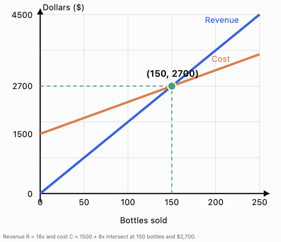
Worked Example: Break-Even Analysis

A company sells reusable bottles for $18 each.

The variable cost is $8 per bottle.

Fixed costs are $1,500.

Find the break-even quantity.

Step 1: Define the variable

x = number of bottles sold

Step 2: Write the revenue equation

R = 18x

Step 3: Write the cost equation

C = 1500 + 8x

Step 4: Set revenue equal to cost

18x = 1500 + 8x

Subtract 8x:

10x = 1500

x = 150

Step 5: Interpret

The company must sell 150 bottles to break even.

Step 6: Verify

Revenue:

R = 18(150) = $2700

Cost:

C = 1500 + 8(150)

C = 1500 + 1200

C = $2700

Revenue equals cost.

Answer: The break-even point is 150 bottles, with revenue and cost both equal to $2,700.

Graphing Break-Even Problems

Break-even analysis can be represented using two straight lines.

One line represents revenue.

The other represents total cost.

The point where the lines intersect is the break-even point.

Interpreting the graph

Before the intersection:

Cost is greater than revenue.

The business operates at a loss.

At the intersection:

Revenue equals cost.

The business breaks even.

After the intersection:

Revenue is greater than cost.

The business earns a profit.

Important assumptions

This linear model assumes that:

• The selling price remains constant.

• Variable cost per unit remains constant.

• Fixed costs remain unchanged.

• All produced units are sold.

• The business has sufficient production capacity.

Real businesses may experience changing prices, discounts, additional costs, and production limits.

Therefore, the model is useful but simplified.

Application: Comparing Two Business Plans

A company is considering two ways to manufacture a product.

Plan A

Fixed costs: $2,000

Variable cost: $5 per unit

Plan B

Fixed costs: $800

Variable cost: $9 per unit

The company wants to know which plan is cheaper at different production levels.

Step 1: Define the variable

x = number of units manufactured

Step 2: Construct the cost equations

Plan A:

Cₐ = 2000 + 5x

Plan B:

Cᵦ = 800 + 9x

Step 3: Find the intersection

At the intersection, both plans have the same cost.

2000 + 5x = 800 + 9x

1200 = 4x

x = 300

Step 4: Calculate the cost

Plan A:

Cₐ = 2000 + 5(300)

Cₐ = $3500

Plan B:

Cᵦ = 800 + 9(300)

Cᵦ = $3500

The two plans cost the same when 300 units are manufactured.

Step 5: Compare different production levels

Business conclusion

Plan B is cheaper for fewer than 300 units because it has lower fixed costs.

Plan A is cheaper for more than 300 units because it has a lower variable cost per unit.

The decision depends on expected production volume.

This example demonstrates how solving a system can identify the point at which one business strategy becomes more economical than another.

Application: Finding Fixed and Variable Costs

A manufacturer records the following production costs:

• Producing 100 units costs $1,400.

• Producing 250 units costs $2,600.

Assuming a linear cost model, determine the fixed cost and variable cost per unit.

Step 1: Define variables

F = fixed cost, in dollars

v = variable cost per unit, in dollars

The model is:

C = F + vx

Step 2: Construct equations

For 100 units:

F + 100v = 1400

For 250 units:

F + 250v = 2600

Step 3: Eliminate F

Subtract the first equation from the second:

150v = 1200

v = 8

Step 4: Find F

F + 100(8) = 1400

F + 800 = 1400

F = 600

Step 5: Interpret

Fixed cost = $600

Variable cost = $8 per unit

Therefore:

C = 600 + 8x

Step 6: Verify

At 100 units:

C = 600 + 8(100) = $1400

At 250 units:

C = 600 + 8(250) = $2600

Both values match the original data.

Business conclusion

The company spends $600 regardless of production volume within the model's operating range, plus $8 for each unit manufactured.

This information can help the business forecast costs at other production levels.

Application: Determining Product Prices from Sales

A school shop sells notebooks and pens.

On Monday, it sells 30 notebooks and 20 pens for $190.

On Tuesday, it sells 20 notebooks and 40 pens for $200.

Find the selling price of each item.

Step 1: Define variables

n = selling price of one notebook

p = selling price of one pen

Step 2: Construct equations

Monday:

30n + 20p = 190

Tuesday:

20n + 40p = 200

Step 3: Simplify

Divide the first equation by 10:

3n + 2p = 19

Divide the second equation by 20:

n + 2p = 10

Step 4: Eliminate p

Subtract the second equation from the first:

2n = 9

n = 4.50

Step 5: Find p

4.50 + 2p = 10

2p = 5.50

p = 2.75

Step 6: Verify

Monday:

30(4.50) + 20(2.75)

= 135 + 55 = $190

Tuesday:

20(4.50) + 40(2.75)

= 90 + 110 = $200

Answer: Notebooks sell for $4.50 and pens sell for $2.75.

Economic interpretation

The system determines the prices that are consistent with both days' sales records, assuming the prices were unchanged and the recorded revenue came only from these items.

Application: Three Products and Total Revenue

A company sells three products: A, B, and C.

Their selling prices are:

• Product A: $10

• Product B: $15

• Product C: $20

During one day, the company sells 100 products and earns $1,500.

It sells 20 more units of Product A than Product C.

Find the quantity of each product sold.

Step 1: Define variables

a = number of Product A units

b = number of Product B units

c = number of Product C units

Step 2: Construct equations

Total units:

a + b + c = 100

Revenue:

10a + 15b + 20c = 1500

Relationship:

a − c = 20

Step 3: Eliminate a

Multiply the total quantity equation by 10:

10a + 10b + 10c = 1000

Subtract from the revenue equation:

5b + 10c = 500

Divide by 5:

b + 2c = 100

Step 4: Use the third equation

a = c + 20

Substitute into the total quantity equation:

c + 20 + b + c = 100

b + 2c = 80

Step 5: Interpret the contradiction

The system requires both:

b + 2c = 100

and:

b + 2c = 80

These cannot both be true.

Therefore, the sales records are inconsistent.

Answer: No solution exists for the stated information.

What could this mean for the business?

Possible explanations include incorrect sales totals, inaccurate revenue records, or an incorrect statement about the relationship between products A and C.

A system of equations can therefore help identify problems in business data, not just calculate unknown quantities.

A consistent version

Suppose the revenue was $1,400 rather than $1,500.

The revenue equation becomes:

10a + 15b + 20c = 1400

Subtracting 10 times the quantity equation gives:

b + 2c = 80

This is the same relationship obtained from a = c + 20.

The revised system has infinitely many solutions, not one unique solution.

An additional independent piece of information would be required to determine the exact quantities.

This illustrates an important limitation: three equations do not guarantee a unique solution if some equations contain redundant information.

Application: Production Planning with Three Products

A factory produces three types of furniture: chairs, tables, and shelves.

Each product requires a different amount of assembly time.

The factory manufactures 100 items using 290 assembly-hours.

It manufactures 10 more chairs than shelves.

Determine the number of each product.

Step 1: Define variables

c = chairs manufactured

t = tables manufactured

s = shelves manufactured

Step 2: Construct equations

Total items:

c + t + s = 100

Total assembly time:

2c + 4t + 3s = 290

Quantity relationship:

c − s = 10

Step 3: Eliminate c

Multiply the first equation by 2:

2c + 2t + 2s = 200

Subtract from the assembly-time equation:

2t + s = 90

Step 4: Use the relationship

c = s + 10

Substitute into the total quantity equation:

s + 10 + t + s = 100

t + 2s = 90

Step 5: Solve the reduced system

We have:

2t + s = 90

t + 2s = 90

Multiply the second equation by 2:

2t + 4s = 180

Subtract the first equation:

3s = 90

s = 30

Then:

t + 2(30) = 90

t = 30

And:

c = 30 + 10 = 40

Step 6: Verify

Total items:

40 + 30 + 30 = 100

Assembly time:

2(40) + 4(30) + 3(30)

= 80 + 120 + 90

= 290 hours

Quantity relationship:

40 − 30 = 10

Answer: 40 chairs, 30 tables, and 30 shelves.

Business conclusion

The factory's production records are consistent with manufacturing 40 chairs, 30 tables, and 30 shelves.

This information could be used to estimate material requirements, labour costs, and future production capacity.

Application: Profit Targets

A business sells handmade bags for $35 each.

The variable cost is $15 per bag.

Monthly fixed costs are $2,400.

The owner wants to earn a monthly profit of $1,600.

How many bags must be sold?

Step 1: Define the variable

x = number of bags sold

Step 2: Write the revenue equation

R = 35x

Step 3: Write the cost equation

C = 2400 + 15x

Step 4: Write the profit equation

P = R − C

P = 35x − (2400 + 15x)

P = 20x − 2400

Step 5: Set the target profit

1600 = 20x − 2400

4000 = 20x

x = 200

Step 6: Verify

Revenue:

35(200) = $7000

Total cost:

2400 + 15(200) = $5400

Profit:

7000 − 5400 = $1600

Answer: The business must sell 200 bags to achieve the target profit of $1,600.

Understanding Contribution Margin

The contribution margin per unit is the selling price minus the variable cost per unit.

Contribution margin = p − v

For this business:

35 − 15 = $20 per bag

Each bag sold contributes $20 toward covering fixed costs and generating profit.

This allows us to write:

P = (p − v)x − F

For a target profit T:

x = (F + T)/(p − v)

provided p − v is positive.

In this example:

x = (2400 + 1600)/(35 − 15)

x = 4000/20

x = 200 bags

When the answer is not a whole number

Suppose the calculation gives:

x = 152.4

If x represents complete products, the business generally needs to sell at least 153 products to reach or exceed its target, assuming the contribution margin is positive.

Rounding down would not achieve the required profit.

Application: Comparing Profit Between Two Businesses

Two businesses sell the same type of product.

Business A has:

• Selling price: $25 per unit

• Variable cost: $10 per unit

• Fixed cost: $1,500

Business B has:

• Selling price: $25 per unit

• Variable cost: $7 per unit

• Fixed cost: $2,400

At what sales volume do the businesses earn the same profit?

Step 1: Construct the profit equations

Business A:

Pₐ = 25x − (1500 + 10x)

Pₐ = 15x − 1500

Business B:

Pᵦ = 25x − (2400 + 7x)

Pᵦ = 18x − 2400

Step 2: Set the profits equal

15x − 1500 = 18x − 2400

900 = 3x

x = 300

Step 3: Calculate the profit

Business A:

Pₐ = 15(300) − 1500 = $3000

Business B:

Pᵦ = 18(300) − 2400 = $3000

Both businesses earn $3,000 profit at 300 units sold.

Step 4: Interpret

Below 300 units, Business A earns more profit because it has lower fixed costs.

Above 300 units, Business B earns more profit because its variable cost per unit is lower.

Comparison table

Business conclusion

The better business model depends on expected sales volume.

A business expecting relatively low sales may prefer lower fixed costs, while one expecting higher sales may benefit from lower variable costs.

Applications in Economics: Supply and Demand

Systems of equations are also used to model markets.

Two important economic concepts are supply and demand.

Demand

Demand describes how much of a product consumers are willing and able to purchase at different prices.

In a simple linear model, quantity demanded decreases as price increases.

For example:

Qd = 100 − 2p

where:

Qd = quantity demanded

p = price

Supply

Supply describes how much producers are willing and able to sell at different prices.

In a simple linear model, quantity supplied increases as price increases.

For example:

Qs = 20 + 2p

Market Equilibrium

Market equilibrium occurs when:

Qd = Qs

This is the price at which quantity demanded equals quantity supplied in the model.

Worked Example: Finding Equilibrium Price

Demand equation:

Qd = 100 − 2p

Supply equation:

Qs = 20 + 2p

At equilibrium:

100 − 2p = 20 + 2p

80 = 4p

p = 20

Substitute into demand:

Qd = 100 − 2(20)

Qd = 60

Substitute into supply:

Qs = 20 + 2(20)

Qs = 60

Equilibrium price = $20

Equilibrium quantity = 60 units

Interpreting the result

At a price of $20, consumers demand 60 units and producers supply 60 units.

At prices below equilibrium, the model predicts that quantity demanded exceeds quantity supplied.

At prices above equilibrium, the model predicts that quantity supplied exceeds quantity demanded.

Important limitation

Real markets are influenced by many factors, including consumer preferences, competition, income, taxes, and changes in production costs.

Linear supply-and-demand equations are simplified models, not exact predictions of every market.

Application: Comparing Subscription Plans

A business is choosing between two software subscriptions.

Plan A charges:

$50 per month plus $4 per user.

Plan B charges:

$110 per month plus $2 per user.

Find the number of users at which the plans cost the same.

Step 1: Define the variable

x = number of users

Step 2: Construct equations

Plan A:

Cₐ = 50 + 4x

Plan B:

Cᵦ = 110 + 2x

Step 3: Set costs equal

50 + 4x = 110 + 2x

2x = 60

x = 30

Step 4: Verify

Plan A:

50 + 4(30) = $170

Plan B:

110 + 2(30) = $170

Answer: Both plans cost $170 per month for 30 users.

Business interpretation

For fewer than 30 users, Plan A is cheaper.

For more than 30 users, Plan B is cheaper.

At exactly 30 users, both plans have the same monthly cost.

This type of comparison is useful when choosing subscriptions, equipment leases, service providers, or production arrangements.

Using Technology in Business Modelling

Spreadsheets and graphing software are useful for business analysis.

For example, a spreadsheet can calculate revenue, cost, and profit for many different sales volumes.

Consider:

R = 18x

C = 1500 + 8x

P = 10x − 1500

A spreadsheet could generate the following table.

The table makes the break-even point easy to identify.

Using graphing software

You can enter:

y = 18x

y = 1500 + 8x

into Desmos Graphing Calculator or GeoGebra Graphing Calculator.

The intersection represents the break-even point.

Technology is particularly useful when businesses need to compare several scenarios or change assumptions.

Evaluating the Reasonableness of Business Solutions

A mathematical answer must make sense in the business context.

Check 1: Units

If x represents the number of products sold, the answer should be expressed in units, not dollars.

If P represents profit, the answer should be expressed in money.

Check 2: Whole numbers

If a calculation gives:

x = 125.6 products

the business cannot normally sell 0.6 of a complete product.

If the goal is to meet or exceed a minimum profit, round up to 126 products when the model supports doing so.

Check 3: Negative values

A negative profit represents a loss.

However, a negative number of products sold is usually invalid in a simple sales model.

Check 4: Capacity

A company may calculate that it needs to sell 5,000 units to achieve its target.

But if it can only produce 3,000 units, the target cannot be reached under the current model.

Check 5: Model assumptions

A linear model assumes constant rates.

Real businesses may experience:

• Bulk discounts.

• Changes in labour costs.

• Limited production capacity.

• Seasonal demand.

• Changing selling prices.

• Additional fixed costs at higher output levels.

These factors can make a simple linear model less accurate.

Check 6: Verification

Always substitute calculated values into the original equations.

For example, if a system predicts that 40 units of A and 30 units of B generate $1,100:

20(40) + 10(30) = 1100

800 + 300 = 1100

The revenue equation is satisfied.

But other conditions must also be checked.

Communicating Mathematical Conclusions

In business and economics, a numerical answer is often not enough.

A complete conclusion should explain what the result means and how it can support a decision.

Example: Weak conclusion

x = 300

Improved conclusion

The two production plans have equal costs when 300 units are manufactured.

Strong conclusion

The two production plans each cost $3,500 at a production level of 300 units. Plan B is cheaper below 300 units because it has lower fixed costs, while Plan A is cheaper above 300 units because it has lower variable costs. Therefore, the company should consider its expected production volume before choosing a plan.

The final conclusion connects the mathematical result to a practical business decision.

A useful structure

When communicating a business solution, include:

1. Result: State the numerical answer with units.

2. Meaning: Explain what the value represents.

3. Verification: Show that it satisfies the original conditions.

4. Recommendation: Explain what the result suggests.

5. Limitation: Identify any assumptions that could affect the decision.

Common Mistakes

Confusing revenue with profit

Revenue is money received from sales. Profit is revenue minus total costs.

Forgetting fixed costs

A business may lose money even when each product sells for more than its variable production cost.

Using the wrong break-even equation

Break-even occurs when total revenue equals total cost, not when revenue equals variable cost alone.

Mixing prices and quantities

The selling price of a product and the number of products sold are different variables.

Constructing incorrect revenue equations

Revenue is calculated by multiplying price by quantity.

Forgetting to include all products

When several products are sold, total revenue must include the revenue from every product.

Rounding sales quantities incorrectly

When calculating the minimum number of complete units required to reach a profit target, round up when appropriate.

Assuming every system has a unique solution

Some business systems contain redundant or contradictory information.

Ignoring production capacity

A mathematically possible sales target may be impossible with existing resources.

Accepting unrealistic negative quantities

Negative profit may be meaningful, but negative quantities of physical products are generally not.

Failing to explain the result

Business conclusions should describe the meaning of the answer, not just provide a number.

Ignoring assumptions

Constant selling prices and costs may not remain realistic over large production ranges.

Key Terms

• Fixed cost: A cost that remains constant over the relevant production range.

• Variable cost: A cost that changes with production volume.

• Total cost: The combined fixed and variable costs.

• Revenue: Money received from sales.

• Profit: Revenue minus total cost.

• Loss: A negative profit.

• Break-even point: The sales volume at which revenue equals total cost.

• Contribution margin: Selling price minus variable cost per unit.

• Selling price: The amount charged for a product or service.

• Unit cost: The cost associated with one unit.

• Production volume: The number of units manufactured.

• Sales volume: The number of units sold.

• Profit target: A desired amount of profit.

• Cost model: An equation representing how costs depend on production or activity.

• Revenue model: An equation representing income from sales.

• Supply: The quantity producers are willing and able to sell at different prices.

• Demand: The quantity consumers are willing and able to buy at different prices.

• Market equilibrium: The point where quantity supplied equals quantity demanded.

• Constraint: A restriction on possible values or decisions.

• Mathematical model: A representation of a real-world situation using equations.

• Verification: Checking that a solution satisfies the original equations.

• Reasonableness: Evaluating whether a mathematical result makes sense in context.

Key Takeaways

• Systems of equations can model costs, revenue, profit, and production.

• Total cost can be represented by C = F + vx.

• Revenue can be represented by R = px when selling price is constant.

• Profit is calculated using P = R − C.

• Break-even occurs when revenue equals total cost.

• Systems can compare two business plans and identify when their costs or profits are equal.

• Two or more sales records can help determine unknown prices or quantities.

• Three-variable systems can model production involving several products.

• Supply-and-demand systems can determine market equilibrium in simplified economic models.

• Mathematical solutions should be interpreted using appropriate units.

• Business decisions should consider capacity, realistic quantities, and model assumptions.

• Strong conclusions explain what a solution means and how it supports a decision.

Check Your Understanding

Recall and Understanding

1. Explain the difference between fixed costs and variable costs. Give one example of each.

2. Define revenue, cost, and profit.

3. What does the break-even point represent?

4. Explain why a business might prefer a production method with higher fixed costs but lower variable costs.

5. Why should a business evaluate the assumptions of a mathematical model before using it to make decisions?

Cost and Profit Problems

6. A company sells water bottles for $20 each. Variable costs are $8 per bottle, and fixed costs are $1,200.

a. Write the revenue equation.

b. Write the total cost equation.

c. Write the profit equation.

d. Find the break-even quantity.

7. A business sells products for $30 each. Variable costs are $12 per unit, and fixed costs are $1,800.

How many products must be sold to earn a profit of $1,800?

8. A manufacturer has fixed costs of $750 and variable costs of $6 per unit.

Calculate the total cost of producing 200 units.

9. A company records total costs of $1,500 when producing 100 units and $2,700 when producing 300 units.

Assuming a linear cost model, determine the fixed cost and variable cost per unit.

10. A company sells 250 products at $24 each. Total costs are $4,200.

Calculate revenue and profit.

Systems and Business Applications

11. Two companies offer production services.

Plan A: $1,000 fixed cost plus $8 per unit.

Plan B: $400 fixed cost plus $12 per unit.

Find the production quantity at which the plans cost the same.

12. A school sells adult tickets for $15 and student tickets for $10.

A total of 120 tickets are sold, generating $1,500.

Determine the number of each ticket type.

13. A shop sells notebooks and pens.

Three notebooks and two pens cost $23.

Two notebooks and four pens cost $26.

Find the price of each item.

14. A factory manufactures chairs, tables, and shelves.

It produces 100 items using 290 assembly-hours.

Each chair requires 2 hours, each table 4 hours, and each shelf 3 hours.

The factory produces 10 more chairs than shelves.

Determine the number of each product.

15. The demand and supply equations for a product are:

Qd = 120 − 3p

Qs = 20 + 2p

Find the equilibrium price and quantity.

Challenge

16. A company sells a product for $25 per unit. Its fixed costs are $2,000, and its variable costs are $10 per unit.

The company can produce at most 180 units.

Can it achieve a profit of $1,000? Explain using calculations.

17. A business compares two profit models:

Pₐ = 12x − 900

Pᵦ = 15x − 1500

Determine when the profits are equal and which model is better for higher sales volumes.

18. A company sells two products.

Product A sells for $20 and Product B for $30.

The company sells 100 units and earns $2,400.

Find the quantity of each product.

19. A manufacturer calculates that it must sell 175.4 units to reach a profit target.

Explain how the answer should be interpreted if only complete units can be sold.

20. A business reports:

x + y + z = 100

2x + 3y + 4z = 290

x − z = 10

Solve the system and explain what the solution could represent in a production context.

Answers to Check Your Understanding

1. Fixed and variable costs

Fixed costs remain unchanged over the relevant production range, such as monthly rent.

Variable costs change with the number of units produced, such as raw materials or packaging.

2. Revenue, cost, and profit

Revenue is money received from sales.

Cost is money spent to operate the business or produce goods.

Profit is the difference:

P = R − C

3. Break-even point

The break-even point is where total revenue equals total cost.

At this point, profit is zero.

4. Higher fixed costs and lower variable costs

A company with higher fixed costs but lower variable costs may become cheaper at high production volumes.

The lower variable cost can eventually offset the higher fixed cost.

5. Evaluating assumptions

Mathematical models simplify real situations.

For example, a linear model may assume constant selling prices, fixed costs, and variable costs.

If these assumptions do not hold, the model's predictions may become inaccurate.

6. Water bottle business

Given:

Selling price = $20

Variable cost = $8

Fixed cost = $1,200

a. Revenue:

R = 20x

b. Total cost:

C = 1200 + 8x

c. Profit:

P = 20x − (1200 + 8x)

P = 12x − 1200

d. Break-even:

20x = 1200 + 8x

12x = 1200

x = 100

Answer: The business breaks even at 100 bottles.

Verification:

Revenue = 20(100) = $2000

Cost = 1200 + 8(100) = $2000

7. Profit target

Selling price = $30

Variable cost = $12

Fixed cost = $1800

Target profit = $1800

Profit equation:

P = 30x − (1800 + 12x)

P = 18x − 1800

Set the target:

1800 = 18x − 1800

3600 = 18x

x = 200

Answer: 200 products.

Verification:

Revenue = 30(200) = $6000

Cost = 1800 + 12(200) = $4200

Profit = $1800

8. Total production cost

C = F + vx

C = 750 + 6(200)

C = 750 + 1200

Answer: $1,950.

9. Finding fixed and variable costs

Let:

F = fixed cost

v = variable cost per unit

Construct equations:

F + 100v = 1500

F + 300v = 2700

Subtract:

200v = 1200

v = 6

Substitute:

F + 100(6) = 1500

F = 900

Answer: Fixed cost = $900; variable cost = $6 per unit.

Cost equation:

C = 900 + 6x

10. Revenue and profit

Revenue:

R = 250(24)

R = $6000

Profit:

P = R − C

P = 6000 − 4200

Answer: Revenue = $6,000; profit = $1,800.

11. Comparing production plans

Plan A:

Cₐ = 1000 + 8x

Plan B:

Cᵦ = 400 + 12x

Set costs equal:

1000 + 8x = 400 + 12x

600 = 4x

x = 150

Calculate cost:

1000 + 8(150) = $2200

400 + 12(150) = $2200

Answer: Both plans cost $2,200 at 150 units.

Below 150 units, Plan B is cheaper.

Above 150 units, Plan A is cheaper.

12. Ticket sales

Let:

a = adult tickets

s = student tickets

Equations:

a + s = 120

15a + 10s = 1500

Multiply the first equation by 10:

10a + 10s = 1200

Subtract:

5a = 300

a = 60

Then:

s = 120 − 60

s = 60

Answer: 60 adult tickets and 60 student tickets.

Verification:

60 + 60 = 120

15(60) + 10(60) = $1500

13. Notebook and pen prices

Let:

n = notebook price

p = pen price

Equations:

3n + 2p = 23

2n + 4p = 26

Multiply the first equation by 2:

6n + 4p = 46

Subtract the second equation:

4n = 20

n = 5

Substitute:

3(5) + 2p = 23

2p = 8

p = 4

Answer: Notebook = $5; pen = $4.

Verification:

3(5) + 2(4) = 23

2(5) + 4(4) = 26

14. Furniture production

Let:

c = chairs

t = tables

s = shelves

Equations:

c + t + s = 100

2c + 4t + 3s = 290

c − s = 10

From the third equation:

c = s + 10

Substitute into the total quantity equation:

t + 2s = 90

Substitute into the assembly-time equation:

2(s + 10) + 4t + 3s = 290

4t + 5s = 270

Multiply t + 2s = 90 by 4:

4t + 8s = 360

Subtract:

3s = 90

s = 30

Then:

t = 90 − 2(30) = 30

c = 30 + 10 = 40

Answer: 40 chairs, 30 tables, and 30 shelves.

Verification:

40 + 30 + 30 = 100

2(40) + 4(30) + 3(30) = 290

15. Market equilibrium

Demand:

Qd = 120 − 3p

Supply:

Qs = 20 + 2p

At equilibrium:

120 − 3p = 20 + 2p

100 = 5p

p = 20

Substitute:

Q = 120 − 3(20)

Q = 60

Answer: Equilibrium price = $20; equilibrium quantity = 60 units.

Verification:

Demand = 60

Supply = 20 + 2(20) = 60

16. Profit target and capacity

Selling price = $25

Variable cost = $10

Fixed cost = $2000

Maximum production = 180 units

Profit equation:

P = 25x − (2000 + 10x)

P = 15x − 2000

To earn $1000:

1000 = 15x − 2000

3000 = 15x

x = 200

However, the company can only produce 180 units.

Maximum profit at full capacity:

P = 15(180) − 2000

P = 2700 − 2000

P = $700

Answer: No. The company cannot achieve a $1,000 profit under the stated conditions. Its maximum possible profit is $700 if it produces and sells all 180 units.

17. Comparing profit models

Pₐ = 12x − 900

Pᵦ = 15x − 1500

Set equal:

12x − 900 = 15x − 1500

600 = 3x

x = 200

Calculate profit:

Pₐ = 12(200) − 900 = $1500

Pᵦ = 15(200) − 1500 = $1500

Answer: Both models produce $1,500 profit at 200 units.

For more than 200 units, Model B produces greater profit because its profit increases by $15 per additional unit compared with $12 for Model A.

18. Two-product sales

Let:

a = units of Product A

b = units of Product B

Total quantity:

a + b = 100

Revenue:

20a + 30b = 2400

Multiply the first equation by 20:

20a + 20b = 2000

Subtract:

10b = 400

b = 40

Then:

a = 60

Answer: 60 units of Product A and 40 units of Product B.

Verification:

60 + 40 = 100

20(60) + 30(40) = $2400

19. Fractional sales quantity

The calculated quantity is:

x = 175.4

If the business must sell complete units and needs to reach or exceed a profit target, it should round up.

Answer: The business must sell at least 176 units, assuming profit increases with each additional unit and the model remains valid.

Rounding down to 175 would leave the business below its target.

20. Three-product production

Given:

x + y + z = 100

2x + 3y + 4z = 290

x − z = 10

From the third equation:

x = z + 10

Substitute into the first:

(z + 10) + y + z = 100

y + 2z = 90

Substitute into the second:

2(z + 10) + 3y + 4z = 290

3y + 6z = 270

Divide by 3:

y + 2z = 90

Both reduced equations are identical.

Therefore, the system does not have a unique solution.

Let z = t.

Then:

x = t + 10

y = 90 − 2t

The general solution is:

(x, y, z) = (t + 10, 90 − 2t, t)

For nonnegative quantities:

0 ≤ t ≤ 45

If the variables represent complete products, t must be an integer.

For example, one possible production combination is:

x = 40

y = 30

z = 30

Verification:

40 + 30 + 30 = 100

2(40) + 3(30) + 4(30) = 290

40 − 30 = 10

Answer: The system has infinitely many nonnegative real solutions and 46 possible whole-number production combinations.

An additional independent condition would be needed to determine the exact production quantities.

Final Summary

Systems of equations provide a practical foundation for analysing business and economic situations.

They can be used to calculate costs, determine prices, establish profit targets, identify break-even points, compare business strategies, and investigate supply-and-demand relationships.

However, mathematical calculations are only part of effective business decision-making. Results must be verified, interpreted using appropriate units, and evaluated against real-world constraints.

The most valuable business solution is not simply a correct number, but a well-supported conclusion that helps explain a situation and guide a decision.