Systems with Three Variables

Introduction

Systems of equations are used to solve problems involving several unknown quantities. They appear in mathematics, science, engineering, economics, business, and many other fields.

We have already learned how to solve systems using algebraic methods such as substitution and elimination. We have also explored how systems can be represented graphically, with solutions appearing where lines or planes intersect.

Although these manual methods are important, some systems become difficult to solve because they involve complicated coefficients, fractions, decimals, or several variables.

This is where technology becomes especially useful.

Graphing calculators, online graphing tools, spreadsheets, and computer algebra systems can help us:

• Graph equations and identify intersection points.

• Solve systems of two or more variables.

• Check answers obtained using manual methods.

• Investigate systems with no solution or infinitely many solutions.

• Interpret mathematical results in real-world situations.

• Explore how changing an equation affects its solution.

However, technology does not replace mathematical understanding. A calculator may produce an answer, but we still need to understand what the answer represents, whether it is accurate, and whether it makes sense.

Why Use Technology to Solve Systems?

Consider the system:

2x + 3y = 12

x − y = 1

This system can be solved easily by substitution or elimination.

However, consider:

17x + 23y = 146

31x − 19y = 52

The second system is more time-consuming to solve manually.

Technology can help determine the solution quickly and reduce arithmetic errors.

Advantages of technology

Speed: Complex calculations can be completed quickly.

Accuracy: Software can reduce arithmetic mistakes, provided equations are entered correctly.

Visualisation: Graphs help us understand how equations relate to one another.

Verification: We can check manually calculated solutions.

Exploration: We can change coefficients and observe how solutions change.

Larger systems: Computers can solve systems involving many unknowns.

Limitations of technology

Technology also has limitations.

• Incorrectly entered equations produce incorrect results.

• Graphical solutions may be approximate.

• Some systems cannot be solved uniquely.

• Numerical methods may introduce rounding errors.

• Software may display results without explaining the reasoning.

• A mathematically correct answer may be unrealistic in context.

The best approach is to combine mathematical reasoning with technological tools.

Graphing Systems of Two Linear Equations

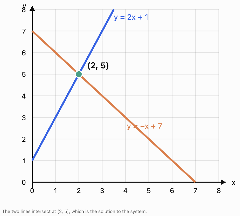
A system of two linear equations can be represented by two lines on the same coordinate plane.

For example:

y = 2x + 1

y = −x + 7

The solution is the point where the lines intersect.

Step 1: Enter the equations

In a graphing calculator or graphing application, enter:

y = 2x + 1

y = −x + 7

Step 2: Display both graphs

The software draws both lines on the same coordinate plane.

Step 3: Locate the intersection

Use the graphing tool's intersection feature, or zoom in and inspect the crossing point.

The intersection is:

(2, 5)

Step 4: Interpret

The x-coordinate is 2.

The y-coordinate is 5.

Therefore:

x = 2

y = 5

Step 5: Verify algebraically

First equation:

5 = 2(2) + 1

5 = 5

Second equation:

5 = −2 + 7

5 = 5

Both equations are satisfied.

Final answer: (2, 5).

Using Desmos to Solve Systems

Desmos Graphing Calculator is a widely used graphing tool that allows users to enter equations and explore their graphs.

You can access it at Desmos Graphing Calculator.

Example

Solve:

3x + 2y = 12

x − y = 1

Step 1: Enter both equations

In Desmos, type:

3x + 2y = 12

x − y = 1

Desmos can graph equations written in standard form, so rearranging them into y = mx + b is not always necessary.

Step 2: Identify the intersection

The lines intersect at:

(2.8, 1.8)

Step 3: Verify

First equation:

3(2.8) + 2(1.8)

= 8.4 + 3.6

= 12

Second equation:

2.8 − 1.8 = 1

Answer: x = 2.8 and y = 1.8.

Why graphing is useful

The graph shows that the two lines cross at exactly one point.

This helps us understand that the system has a unique solution.

Graphing is particularly useful for visualising systems and checking answers.

Understanding Graphing Windows

A graphing window determines which part of the coordinate plane is visible.

For example, suppose:

y = 2x + 100

y = −x + 400

The intersection occurs at:

2x + 100 = −x + 400

3x = 300

x = 100

y = 300

The solution is:

(100, 300)

If the graphing window only displays x-values between −10 and 10 and y-values between −10 and 10, the intersection will not be visible.

This does not mean the system has no solution.

It means the graphing window is too small.

Improving the graph

Adjust the axes to include the expected solution.

For example:

x-axis: 0 to 150

y-axis: 0 to 450

The intersection will then be visible.

Important lesson

A missing intersection on the screen does not necessarily mean that the system has no solution.

Always consider the scale and viewing window.

Using GeoGebra to Solve Systems

GeoGebra is another useful tool for exploring equations and their solutions.

GeoGebra Graphing Calculator

GeoGebra can graph equations, identify intersections, and explore how changing coefficients affects a system.

Worked Example: Two Lines

Solve:

2x + y = 11

x − y = 1

Enter both equations into the graphing calculator.

The two lines intersect at:

(4, 3)

Verification:

2(4) + 3 = 11

4 − 3 = 1

Both equations are satisfied.

Comparing graphing tools

For three-variable systems, use GeoGebra 3D Calculator rather than the ordinary two-dimensional graphing view.

Graphing Systems with No Solution

Consider:

y = 2x + 1

y = 2x − 4

Both equations have the same slope:

m = 2

However, they have different y-intercepts:

1 and −4

Therefore, the lines are parallel.

They never intersect.

A graphing calculator will display two distinct parallel lines.

Answer: No solution.

Verifying algebraically

Set the expressions equal:

2x + 1 = 2x − 4

Subtract 2x:

1 = −4

This is impossible.

The system is inconsistent.

Graphing Systems with Infinitely Many Solutions

Consider:

y = 3x + 2

2y = 6x + 4

Simplify the second equation:

y = 3x + 2

Both equations represent exactly the same line.

The graphs overlap completely.

Every point on the line satisfies both equations.

Answer: Infinitely many solutions.

Interpreting overlapping graphs

Graphing software may display what appears to be only one line.

This does not necessarily mean that one equation failed to graph.

It may mean that both equations represent the same line.

To confirm, simplify both equations algebraically.

Comparing the Three Types of Systems

This classification is particularly useful when interpreting technological outputs.

Solving Three-Variable Systems with Technology

Two-variable systems can be represented by lines in a coordinate plane.

Three-variable linear systems are different.

Each equation generally represents a plane in three-dimensional space.

For example:

x + y + z = 9

2x + y + z = 11

x + 2y + z = 12

Each equation represents a plane.

The solution is the point shared by all three planes.

Worked Example: Three-Variable System

Solve:

x + y + z = 9

2x + y + z = 11

x + 2y + z = 12

Using graphing technology

Enter the equations into a suitable three-dimensional graphing application.

The software displays three planes.

If the planes share exactly one point, the system has a unique solution.

For this system, the common point is:

(2, 3, 4)

Verify manually

First equation:

2 + 3 + 4 = 9

Second equation:

2(2) + 3 + 4 = 11

Third equation:

2 + 2(3) + 4 = 12

All three equations are satisfied.

Confirm using elimination

Subtract the first equation from the second:

x = 2

Subtract the first equation from the third:

y = 3

Substitute into the first:

2 + 3 + z = 9

z = 4

Answer: (2, 3, 4).

The graphical and algebraic methods produce the same solution.

Interpreting Three-Dimensional Graphs

Three-dimensional graphs require careful interpretation because the planes may overlap or intersect in different ways.

One solution

Three planes share exactly one point.

The solution is one ordered triple.

No solution

The three planes have no common point.

For example, two of the planes may be parallel and distinct.

Infinitely many solutions

The planes may share a line or coincide.

In these situations, infinitely many points satisfy the equations.

Important limitation

A three-dimensional picture can be misleading because of perspective, overlapping surfaces, or the selected viewing angle.

A graph may suggest a particular intersection, but algebraic verification is needed to confirm the result.

Using Scientific Calculators

Many scientific calculators contain a simultaneous-equation solver.

For example, some models from Casio and Texas Instruments support solving linear systems.

The exact procedure depends on the calculator model.

A typical workflow is:

1. Select the equation or simultaneous-equation mode.

2. Choose the number of unknowns.

3. Enter the coefficients and constants.

4. Execute the calculation.

5. Read the values of the variables.

6. Substitute the results into the original equations.

Worked Example

Solve:

2x + y − z = 8

x + 2y + z = 7

3x − y + 2z = 7

The coefficients can be organised as follows:

A calculator's simultaneous-equation mode can use these values to solve the system.

The solution is:

x = 3, y = 2, z = 0

Verification:

2(3) + 2 − 0 = 8

3 + 2(2) + 0 = 7

3(3) − 2 + 2(0) = 7

All three equations are satisfied.

Why coefficient tables are useful

Coefficient tables help prevent mistakes when entering equations into a calculator.

They are particularly important when an equation is missing a variable.

For example:

2x + 3z = 10

must be entered as:

2x + 0y + 3z = 10

The coefficient of y is zero.

Forgetting this zero may cause the remaining values to be entered in the wrong positions.

Solving Systems with Spreadsheets

Spreadsheet software such as Microsoft Excel or Google Sheets can also be used to solve systems.

Spreadsheets are especially useful when working with larger sets of equations, repeated calculations, or real-world data.

Representing a system using a matrix

Consider:

2x + y + z = 9

x + 3y + 2z = 13

3x + 2y + z = 11

The coefficients form the matrix:

The constants form another column:

We can represent the system using:

AX = B

where:

A = coefficient matrix

X = column of unknown variables

B = column of constants

Solving with matrix operations

When A is invertible:

X = A⁻¹B

Spreadsheet software can calculate the inverse matrix and multiply it by the constants.

In Excel or Google Sheets, a typical approach is to enter the coefficients in cells A1:C3 and the constants in E1:E3.

Then use:

=MMULT(MINVERSE(A1:C3),E1:E3)

In current spreadsheet versions that support dynamic arrays, the three results can spill into adjacent cells. Older spreadsheet versions may require array-formula entry.

For the example above, the solution is:

x = 2

y = 1

z = 4

Verification:

2(2) + 1 + 4 = 9

2 + 3(1) + 2(4) = 13

3(2) + 2(1) + 4 = 12

The third equation does not equal 11.

Therefore, the proposed values are not the solution.

The correct spreadsheet result is:

x = 3/2, y = −1/2, z = 13/2

Check:

2(3/2) − 1/2 + 13/2 = 9

3/2 + 3(−1/2) + 2(13/2) = 13

3(3/2) + 2(−1/2) + 13/2 = 10

This also fails the third equation.

We therefore need to solve the system carefully rather than accepting an unverified result.

Using elimination:

From the first equation:

z = 9 − 2x − y

Substitute into the second:

x + 3y + 2(9 − 2x − y) = 13

−3x + y = −5

y = 3x − 5

Substitute into the third:

3x + 2y + 9 − 2x − y = 11

x + y = 2

Substitute y = 3x − 5:

x + 3x − 5 = 2

4x = 7

x = 7/4

Then:

y = 3(7/4) − 5

y = 1/4

And:

z = 9 − 2(7/4) − 1/4

z = 21/4

Verification:

2(7/4) + 1/4 + 21/4 = 9

7/4 + 3(1/4) + 2(21/4) = 13

3(7/4) + 2(1/4) + 21/4 = 11

Correct solution: (7/4, 1/4, 21/4).

This example illustrates why verification remains essential, even when technology is involved.

When matrix methods cannot be used directly

The inverse-matrix formula requires an invertible square coefficient matrix.

If the matrix is singular, the inverse does not exist.

This may happen when the equations are dependent or when the system does not have a unique solution.

A calculator or spreadsheet may display an error rather than three numerical values.

That error does not automatically tell us whether the system has no solution or infinitely many solutions.

Further analysis is required.

Comparing Manual and Technological Methods

Different methods have different strengths.

When should technology be used?

Technology is particularly helpful when:

• Coefficients are large or contain fractions.

• A system has three or more unknowns.

• Many similar systems must be solved.

• A graph would improve understanding.

• Manual calculations need checking.

• The effects of changing coefficients are being investigated.

Manual methods are especially useful when the purpose is to understand how the equations work or to explain why a solution exists.

Technology is most effective when it supports mathematical reasoning rather than replacing it.

Worked Example: Comparing Manual and Calculator Solutions

Solve:

4x + 3y = 19

2x − 5y = −13

Manual method

Multiply the second equation by 2:

4x − 10y = −26

Subtract from the first equation:

13y = 45

y = 45/13

Substitute into the first equation:

4x + 3(45/13) = 19

4x = 247/13 − 135/13

4x = 112/13

x = 28/13

Exact solution: (28/13, 45/13).

Calculator method

A calculator may display:

x ≈ 2.153846

y ≈ 3.461538

These are decimal approximations of the same solution.

Comparing the outputs

The manual method gives exact fractions.

The calculator provides convenient decimal values.

Both are useful, but exact fractions are preferable when further algebraic calculations are required.

Technology and Rounding Errors

Computers and calculators often represent numbers using a limited number of decimal places.

Suppose a calculator displays:

x = 1.333333

The exact value might be:

x = 4/3

If we substitute the rounded decimal into an equation, the result may be slightly different from the expected constant.

For example:

3(1.333333) = 3.999999

rather than exactly 4.

This small difference is caused by rounding.

Good practice

Keep exact values when possible.

If decimal approximations are required, retain sufficient precision during calculations and round only the final result.

A very small numerical difference may be acceptable, but a large discrepancy usually indicates an error.

Technology in Real-World Applications

Business and Economics

A business can use spreadsheets to solve systems involving product quantities, prices, revenue, and production costs.

Engineering

Engineers use computer software to solve systems describing forces, electrical circuits, and structural behaviour.

Science

Scientists use systems of equations to analyse experimental data, mixtures, and physical relationships.

Transport

Transport planners can use mathematical models to analyse vehicle movement, scheduling, and resource allocation.

Computer Graphics

Three-dimensional computer graphics use systems of equations and matrix calculations to represent and transform objects.

Common Mistakes

Entering equations incorrectly

A missing negative sign or coefficient can completely change the answer.

Using an inappropriate graphing window

An intersection may exist outside the visible region.

Assuming two lines do not intersect because they appear parallel

Lines with very similar slopes may intersect far away.

Treating approximate values as exact

Graphical and numerical solutions may be rounded.

Confusing the coordinates

The solution (3, 5) means x = 3 and y = 5, not the reverse.

Assuming every calculator error means no solution

Some errors indicate a singular matrix or unsupported calculation rather than an inconsistent system.

Using a two-dimensional graphing tool for three-dimensional equations

Three-variable systems generally require a three-dimensional graphing application or another solving method.

Accepting a technological output without checking it

Always substitute the proposed values into the original equations.

Ignoring real-world restrictions

Negative quantities or fractional counts may be mathematically possible but contextually invalid.

Key Terms

• Graphing calculator: A device or application that displays mathematical graphs.

• Graphing software: Computer software used to represent equations visually.

• Intersection point: A point shared by two or more graphs.

• Simultaneous equations: Equations solved together to determine common variable values.

• Numerical solution: A solution expressed using numerical values, often approximations.

• Exact solution: A solution expressed without rounding.

• Approximation: A value close to, but not necessarily equal to, an exact value.

• Graphing window: The range of coordinates displayed on a graph.

• Matrix: A rectangular arrangement of numbers.

• Coefficient matrix: A matrix containing the coefficients of a system.

• Inverse matrix: A matrix that reverses the effect of multiplication by an invertible matrix.

• Singular matrix: A square matrix that does not have an inverse.

• Computer algebra system: Software capable of performing symbolic mathematical operations.

• Verification: Checking that a proposed solution satisfies the original equations.

• Consistent system: A system with at least one solution.

• Inconsistent system: A system with no solution.

• Dependent equations: Equations that contain redundant information.

• Rounding error: A small numerical difference caused by using approximate values.

Key Takeaways

• Technology can help solve and visualise systems of equations.

• Graphing software identifies solutions as intersection points.

• Two-variable linear systems are represented by lines.

• Three-variable linear systems are represented by planes.

• Scientific calculators can solve systems using coefficients and constants.

• Spreadsheets can use matrices to solve linear systems.

• Exact algebraic solutions and approximate numerical solutions should be distinguished.

• Graphing windows must be chosen carefully.

• Technology can reveal whether systems have one, no, or infinitely many solutions, although further analysis may be needed.

• Manual methods remain important for understanding and explaining mathematical relationships.

• Every technological solution should be verified using the original equations.

Check Your Understanding

Recall and Understanding

1. Explain two advantages of using technology to solve systems of equations.

2. What does the intersection of two lines represent?

3. Why might a graphing calculator fail to display an intersection even when one exists?

4. Explain the difference between an exact solution and an approximate solution.

5. Why is verification necessary when using technology?

Application

6. Use a graphing calculator or algebraic method to solve:

y = 2x + 3

y = −x + 12

7. Solve and verify:

3x + 2y = 16

x − y = 2

8. Determine the number of solutions:

y = 4x + 1

y = 4x − 3

9. Determine the number of solutions:

2x + 4y = 12

x + 2y = 6

10. Solve the three-variable system:

x + y + z = 12

2x + y + z = 15

x + 2y + z = 16

Analysis and Challenge

11. A graphing calculator displays the intersection (2.6667, 3.3333). Explain why these coordinates may not be exact.

12. A student enters the system:

2x + 3y = 12

x − y = 1

The calculator gives x = 3 and y = 2. Verify whether this is correct.

13. Explain why a system with dependent equations may cause a matrix-inverse calculation to fail.

14. A calculator produces x = −5, y = 20, z = 15 for a ticket-sales problem. Explain what should be checked before accepting the result.

15. Solve using a calculator, spreadsheet, or elimination:

2x + y + z = 9

x + 3y + 2z = 13

3x + 2y + z = 11

Answers to Check Your Understanding

1. Technology can perform complicated calculations quickly and display graphs that help us understand the relationships between equations.

2. The intersection represents the ordered pair that satisfies both equations simultaneously.

3. The intersection may lie outside the selected graphing window.

4. An exact solution is not rounded, such as 4/3. An approximate solution is a numerical estimate, such as 1.3333.

5. Equations may have been entered incorrectly, numerical results may be rounded, or the output may not make sense in the original context.

6.

Set the equations equal:

2x + 3 = −x + 12

3x = 9

x = 3

Then:

y = 2(3) + 3 = 9

Answer: (3, 9).

7.

3x + 2y = 16

x − y = 2

From the second equation:

x = y + 2

Substitute:

3(y + 2) + 2y = 16

5y + 6 = 16

y = 2

x = 4

Verification:

3(4) + 2(2) = 16

4 − 2 = 2

Answer: (4, 2).

8. No solution. The lines have the same slope but different y-intercepts.

9. Infinitely many solutions. The second equation multiplied by 2 gives the first equation, so both represent the same line.

10.

x + y + z = 12

2x + y + z = 15

x + 2y + z = 16

Subtract the first equation from the second:

x = 3

Subtract the first equation from the third:

y = 4

Substitute:

3 + 4 + z = 12

z = 5

Answer: (3, 4, 5).

11. The calculator may have rounded the coordinates. The exact values could be fractions such as 8/3 and 10/3.

12.

Check the first equation:

2(3) + 3(2) = 12

Correct.

Check the second:

3 − 2 = 1

Correct.

Answer: (3, 2) is a valid solution.

13. Dependent equations can produce a singular coefficient matrix. A singular matrix has no inverse, so the inverse-matrix method cannot be applied directly.

14. The values should be substituted into the original equations. Since x = −5, the result is invalid if x represents a number of tickets. Ticket quantities must be nonnegative whole numbers.

15.

The system is:

2x + y + z = 9

x + 3y + 2z = 13

3x + 2y + z = 11

From the first equation:

z = 9 − 2x − y

Substitute into the second:

x + 3y + 2(9 − 2x − y) = 13

−3x + y = −5

y = 3x − 5

Substitute into the third:

3x + 2y + 9 − 2x − y = 11

x + y = 2

Substitute y = 3x − 5:

4x − 5 = 2

x = 7/4

Then:

y = 3(7/4) − 5 = 1/4

And:

z = 9 − 2(7/4) − 1/4 = 21/4

Verification:

2(7/4) + 1/4 + 21/4 = 9

7/4 + 3(1/4) + 2(21/4) = 13

3(7/4) + 2(1/4) + 21/4 = 11

Answer: (7/4, 1/4, 21/4).

Final Summary

Graphing calculators, mathematical software, and spreadsheets provide powerful ways to solve systems of equations and investigate their properties.

Technology is particularly valuable for complex calculations, visualising intersections, and checking answers. However, understanding substitution, elimination, and the meaning of solutions remains essential.

The most effective mathematical problem-solving combines the efficiency of technology with the accuracy, interpretation, and reasoning provided by algebraic methods.