Analyzing and Interpreting Graphs
5. Function Modeling Project
Learning outcomes
- I can collect data from a real-world situation.
- I can select an appropriate function model.
- I can create equations and graphs.
- I can interpret the results of my model.
- I can communicate my findings using mathematical language.
Introduction
Mathematics is not only about solving equations and drawing graphs. It is also a powerful tool for understanding real-world situations, identifying patterns, making predictions, and solving practical problems.
For example, mathematical functions can help us investigate questions such as:
-
How does the height of a bouncing ball change over time?
-
How quickly does a plant grow?
-
How does the cost of a taxi journey depend on the distance travelled?
-
How does the temperature of a hot drink change as it cools?
-
How does the area of a rectangle change when its dimensions change?
-
How can we predict future population growth?
These questions can be investigated through mathematical modelling.
Mathematical modelling is the process of representing a real-world situation using mathematical ideas such as equations, functions, tables, and graphs.
A mathematical model does not need to describe reality perfectly. Instead, it should capture the important relationships in a situation accurately enough to explain observations, make useful predictions, or support decisions.
In this project, we will explore how to collect data, identify patterns, select suitable functions, construct mathematical models, interpret results, and communicate conclusions.
What Is Mathematical Modelling?
A mathematical model is a simplified mathematical representation of a real-world situation.
Models may include:
-
Equations.
-
Functions.
-
Tables of values.
-
Graphs.
-
Diagrams.
-
Statistical relationships.
For example, suppose a bicycle rental company charges a fixed fee of $5 plus $3 per hour.
The total cost can be represented by:
C = 3h + 5
where:
-
C is the total cost in dollars.
-
h is the number of hours rented.
This equation is a mathematical model.
It allows us to calculate the rental cost for different durations.
For example, for 4 hours:
C(4) = 3(4) + 5
C(4) = 17
The total cost is $17.
The model also helps us understand the relationship:
-
The cost increases by $3 for every additional hour.
-
The initial fee is $5.
-
The relationship is linear.
-
The graph is a straight line.
A useful mathematical model should explain the observed relationship and make predictions that are reasonable within the situation being studied.
The Mathematical Modelling Cycle
Mathematical modelling is a process that often involves several stages.
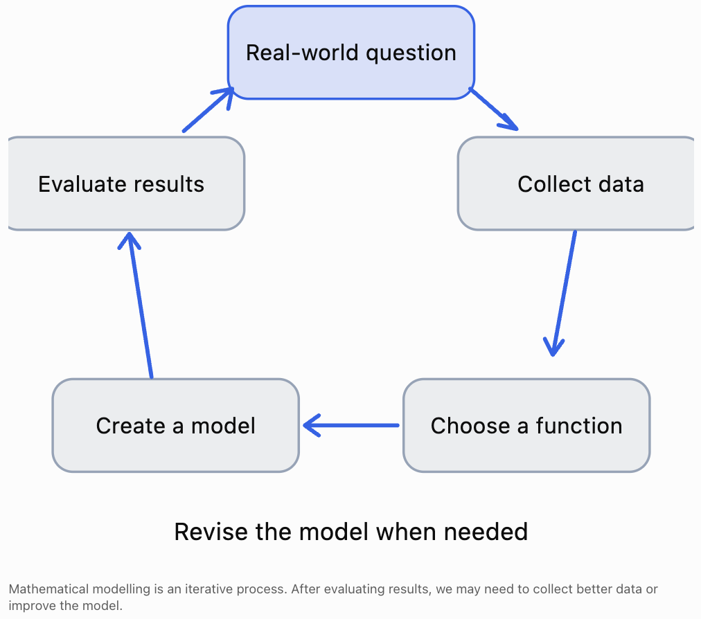
A typical modelling project follows these stages:
-
Identify a real-world question.
-
Decide which variables to investigate.
-
Collect reliable data.
-
Organise the data in tables and graphs.
-
Identify patterns.
-
Select an appropriate function.
-
Construct an equation.
-
Compare the model with the observed data.
-
Interpret results and make predictions.
-
Communicate findings and evaluate limitations.
The process is not always completed in a straight line.
For example, after plotting the data, we may realise that the original measurements were insufficient or that another function would describe the situation more accurately.
Revising a model is a normal and important part of mathematical investigation.
Choosing a Real-World Situation
The first stage of a modelling project is selecting a situation that can be investigated mathematically.
A suitable project should involve two quantities that can be measured or calculated.
Examples include:
|
Project idea |
Independent variable |
Dependent variable |
Possible function |
|---|---|---|---|
|
Bicycle rental cost |
Time |
Cost |
Linear |
|
Plant growth |
Time |
Height |
Linear, logistic, or another growth model |
|
Cooling drink |
Time |
Temperature |
Exponential decay toward room temperature |
|
Ball thrown upward |
Time |
Height |
Quadratic |
|
Square area |
Side length |
Area |
Quadratic |
|
Savings with compound interest |
Time |
Account balance |
Exponential growth |
|
Walking at steady speed |
Time |
Distance |
Linear |
|
Sound intensity with distance |
Distance |
Intensity |
Inverse-square relationship |
|
Seasonal temperature |
Time |
Temperature |
Periodic or sinusoidal |
|
Braking distance |
Speed |
Braking distance |
Approximately quadratic under fixed conditions |
The choice of function should depend on the observed relationship, not simply on the topic.
For example, plant growth may appear approximately linear over a short period but may slow down as the plant approaches its mature size.
Identifying Variables
A mathematical model usually describes how one variable depends on another.
Independent variable
The independent variable is the input.
It is often represented by x.
Examples include:
-
Time.
-
Distance travelled.
-
Number of products sold.
-
Side length.
-
Temperature.
Dependent variable
The dependent variable is the output.
It is often represented by y or f(x).
Examples include:
-
Total cost.
-
Height.
-
Profit.
-
Area.
-
Population.
Worked Example
Suppose we investigate how the distance travelled by a toy car changes over time.
The independent variable is:
Time (seconds)
The dependent variable is:
Distance travelled (metres)
We can write:
d = f(t)
This means that distance is modelled as a function of time.
Controlled conditions
In practical investigations, other variables may influence the results.
For example, when measuring toy car motion, we should consider:
-
Whether the car moves on the same surface.
-
Whether the starting position remains the same.
-
Whether the car travels along a straight path.
-
Whether the method of measuring time is consistent.
Controlling these conditions helps make the data more reliable.
Collecting Real-World Data
Reliable data is essential for developing a useful mathematical model.
Data can be collected through:
-
Direct measurements.
-
Scientific experiments.
-
Surveys.
-
Observations.
-
Public datasets.
-
Digital sensors.
-
Simulations.
Example: Measuring the motion of a toy car
Suppose a toy car travels along a straight track.
We record its distance from the starting point at regular time intervals.
The following is an illustrative dataset, not actual experimental measurements.
|
Time (s) |
Distance (m) |
|---|---|
|
0 |
0.0 |
|
1 |
1.5 |
|
2 |
3.1 |
|
3 |
4.4 |
|
4 |
6.2 |
|
5 |
7.6 |
|
6 |
9.1 |
The data suggests that distance increases approximately linearly with time.
However, the measurements are not perfectly aligned.
This could be caused by:
-
Measurement uncertainty.
-
Small changes in speed.
-
Human reaction time.
-
Surface friction.
-
Differences in how the car was released.
Real-world data often contains variation.
A mathematical model should describe the overall trend rather than necessarily passing through every measurement.
Organising Data in Tables
A data table should be clear and easy to interpret.
A good table includes:
-
Descriptive headings.
-
Correct units.
-
Consistent numerical precision.
-
Measurements arranged logically.
-
Enough observations to identify patterns.
For example:
|
Time (s) |
Distance (m) |
|---|---|
|
0 |
0.0 |
|
1 |
1.5 |
|
2 |
3.1 |
|
3 |
4.4 |
Avoid using headings such as simply "x" and "y" in a final scientific report when meaningful variable names are available.
Instead, write:
Time (s) and Distance (m)
This makes the data understandable to someone who did not conduct the experiment.
Creating Scatter Plots
A scatter plot represents pairs of measured values on a coordinate plane.
Each point represents one observation.
For the toy car experiment:
-
Time is placed on the horizontal axis.
-
Distance is placed on the vertical axis.
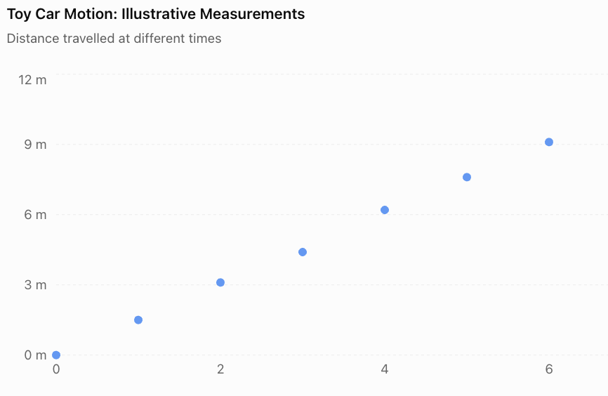
The plotted points show an upward trend.
This suggests that distance increases as time increases.
The points are also approximately arranged along a straight line.
Therefore, a linear function may be a suitable model.
Important distinction
A scatter plot shows the observed measurements.
A model graph represents the mathematical relationship used to describe those measurements.
The two should be compared, but they are not necessarily identical.
Recognising Function Patterns
One of the most important modelling skills is recognising the shape of a relationship.
Different function families produce different patterns.
Linear relationships
A linear function has the form:
y = mx + c
Its graph is a straight line.
A linear model is appropriate when the dependent variable changes by approximately the same amount for equal increases in the independent variable.
Examples include:
-
Distance travelled at constant speed.
-
Cost with a fixed fee and constant rate.
-
Earnings at a fixed hourly wage.
Quadratic relationships
A quadratic function has the form:
y = ax² + bx + c
Its graph is a parabola.
Quadratic models are useful when the rate of change changes approximately linearly with the input.
Examples include:
-
Height of a projectile under constant gravitational acceleration.
-
Area as a function of side length.
-
Some simplified profit and revenue models.
Exponential relationships
An exponential function has the form:
y = abˣ
where a ≠ 0, b > 0, and b ≠ 1.
Exponential models are useful when a quantity changes by approximately the same percentage over equal input intervals.
Examples include:
-
Compound interest.
-
Idealised population growth.
-
Radioactive decay.
-
Cooling toward a constant surrounding temperature, using a shifted exponential model.
Inverse relationships
An inverse function may have the form:
y = k/x
where x ≠ 0.
Examples include:
-
Time required to travel a fixed distance at different speeds.
-
Pressure and volume of an ideal gas at constant temperature, under suitable conditions.
Periodic relationships
Periodic functions repeat patterns over regular intervals.
Sine and cosine functions are commonly used:
y = A sin(B(x − h)) + k
Examples include:
-
Oscillations.
-
Seasonal patterns.
-
Tides.
-
Rotating machinery.
Comparing Function Families
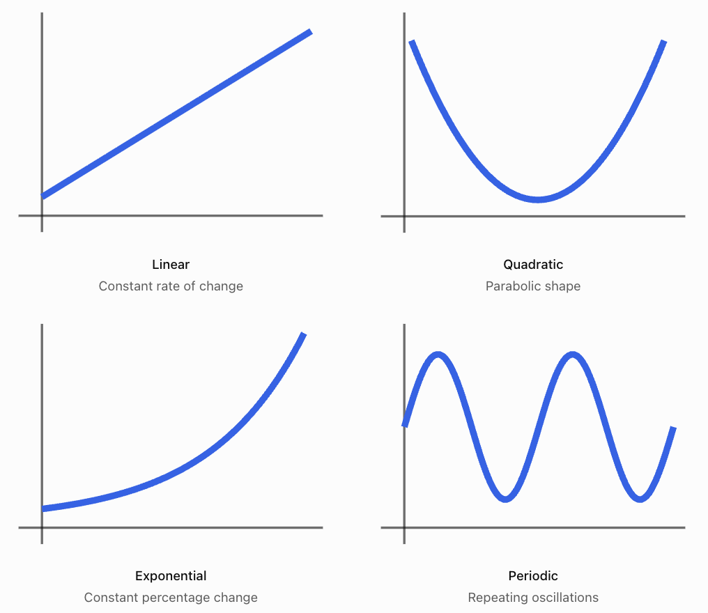
These graph shapes help us select possible models, but visual appearance alone is not enough.
We must also consider the context, mathematical assumptions, and how well the model matches the data.
Creating a Linear Model from Data
Return to the toy car measurements.
Suppose we estimate a line using two representative points:
(0, 0) and (6, 9.1)
The gradient is:
m = (y₂ − y₁)/(x₂ − x₁)
Substitute:
m = (9.1 − 0)/(6 − 0)
m ≈ 1.52
The y-intercept is approximately zero.
Therefore, a simple linear model is:
d(t) = 1.52t
where:
-
d is distance in metres.
-
t is time in seconds.
Interpreting the gradient
The gradient represents speed.
A gradient of 1.52 means the toy car travels approximately 1.52 metres per second under this model.
Making a prediction
How far will the car travel after 8 seconds?
d(8) = 1.52(8)
d(8) = 12.16
Predicted distance ≈ 12.16 m
This prediction assumes the car continues moving at approximately the same speed.
Evaluating the model
The model predicts:
Time (s)
Measured distance (m)
Predicted distance (m)
0
0.0
0.00
1
1.5
1.52
2
3.1
3.04
3
4.4
4.56
4
6.2
6.08
5
7.6
7.60
6
9.1
9.12
The predictions are reasonably close to the illustrative measurements.
This supports using a linear model over the observed interval.
However, the line was estimated from selected points rather than calculated using formal regression.
A least-squares regression line could provide a more systematic fit.
Residuals and Model Accuracy
A residual is the difference between an observed value and the value predicted by a model.
Residual = Observed value − Predicted value
Worked Example
At t = 3 seconds:
Observed distance = 4.4 m
Predicted distance = 1.52(3) = 4.56 m
Residual:
4.4 − 4.56 = −0.16 m
The negative residual means the model overestimated the observed distance by 0.16 m.
Interpreting residuals
-
Positive residual: the observed value is above the prediction.
-
Negative residual: the observed value is below the prediction.
-
Zero residual: the prediction matches the observation.
A good model generally has relatively small residuals with no strong systematic pattern.
If residuals consistently form a curve, a different function family may be more suitable.
A model with very small residuals is not automatically the best model, however. It must also make sense in the real-world situation and avoid unnecessary complexity.
Creating a Quadratic Model
Suppose we investigate the height of a ball thrown vertically upward.
Under a simplified model with constant gravitational acceleration and negligible air resistance:
h(t) = −4.9t² + v₀t + h₀
where:
-
h(t) = height in metres.
-
t = time in seconds.
-
v₀ = initial vertical velocity in metres per second.
-
h₀ = initial height in metres.
Suppose the ball is released from a height of 1.5 m with an initial upward velocity of 14.7 m/s.
Then:
h(t) = −4.9t² + 14.7t + 1.5
Finding the maximum height
The vertex occurs at:
t = −b/(2a)
Here:
a = −4.9
b = 14.7
Therefore:
t = −14.7/[2(−4.9)]
t = 1.5 s
Substitute:
h(1.5) = −4.9(1.5)² + 14.7(1.5) + 1.5
h(1.5) = −11.025 + 22.05 + 1.5
h(1.5) = 12.525
Maximum height ≈ 12.53 m
The ball reaches its maximum height after 1.5 seconds.
Finding when the ball reaches the ground
Set h(t) = 0:
0 = −4.9t² + 14.7t + 1.5
Using the quadratic formula, the positive solution is approximately:
t ≈ 3.10 s
The ball reaches the ground approximately 3.10 seconds after release.
Interpreting the model
The model predicts that:
-
The ball begins 1.5 m above the ground.
-
It rises until t = 1.5 s.
-
Its maximum height is approximately 12.53 m.
-
It then falls.
-
It reaches the ground at approximately 3.10 s.
The practical domain is approximately:
0 ≤ t ≤ 3.10
The model should not be used to predict the ball's height long after it hits the ground.
Creating an Exponential Model
Suppose a population of microorganisms starts at 200 and increases by 15% every hour.
The population can be modeled by:
P(t) = 200(1.15)ᵗ
where t is time in hours.
Understanding the equation
-
200 is the initial population.
-
1.15 is the growth factor.
-
0.15 represents a 15% increase per hour.
-
t is the number of hours.
Making predictions
After 4 hours:
P(4) = 200(1.15)⁴
P(4) ≈ 349.8
The model predicts approximately 350 microorganisms.
After 8 hours:
P(8) = 200(1.15)⁸
P(8) ≈ 611.8
The model predicts approximately 612 microorganisms.
Evaluating the model
Exponential growth may describe a population over a limited period.
However, real populations cannot increase indefinitely without constraints.
Factors such as food supply, space, competition, and waste accumulation may eventually slow growth.
Therefore, the model may be useful for short-term predictions but unsuitable for very long-term predictions.
Interpolation and Extrapolation
Models can be used to estimate values that were not directly measured.
Two important terms are interpolation and extrapolation.
Interpolation
Interpolation means estimating a value within the range of collected data.
For example, suppose we measured a car's distance between 0 and 6 seconds.
Using the model to estimate distance at 2.5 seconds is interpolation.
d(2.5) = 1.52(2.5)
d(2.5) = 3.8 m
Extrapolation
Extrapolation means predicting beyond the range of collected data.
Using the same model to estimate distance after 20 seconds is extrapolation.
d(20) = 1.52(20)
d(20) = 30.4 m
However, this prediction may be unreliable if the car slows down, changes direction, or reaches the end of the track.
Extrapolation generally requires greater caution because the relationship may change beyond the observed data.
Using Technology to Build Models
Digital tools make mathematical modelling easier.
Common options include:
-
Desmos — plotting functions and using regression tools.
-
GeoGebra — graphing, regression, and mathematical exploration.
-
Microsoft Excel — organising data, scatter plots, and trendlines.
-
Google Sheets — tables, charts, and regression calculations.
Example workflow using a spreadsheet
-
Enter the independent variable in the first column.
-
Enter the dependent variable in the second column.
-
Highlight the data.
-
Insert a scatter plot.
-
Add a trendline.
-
Choose a suitable model type.
-
Display the trendline equation when supported.
-
Compare the predicted values with the measurements.
-
Use the equation to make predictions.
Technology helps us fit models more efficiently, but we must still decide whether the model makes mathematical and practical sense.
Evaluating a Mathematical Model
A mathematical model should be evaluated rather than accepted automatically.
Useful evaluation questions include:
-
Does the model describe the observed data accurately?
-
Does the equation have a reasonable interpretation?
-
Are the units correct?
-
Does the model follow the expected scientific or mathematical relationship?
-
Are there large differences between observed and predicted values?
-
Is the model suitable for predictions outside the observed interval?
-
What assumptions were made?
-
What factors were ignored?
-
Could a different function provide a better model?
Accuracy versus usefulness
A model does not have to match every observation perfectly to be useful.
For example, a linear model may describe the motion of a toy car well enough to estimate its average speed, even if small variations occur in the measurements.
However, if the car accelerates significantly, a quadratic model may provide a better description of distance over time.
Model limitations
All mathematical models simplify reality.
Possible limitations include:
-
Measurement uncertainty.
-
Small sample sizes.
-
Uncontrolled variables.
-
Changes in environmental conditions.
-
Incorrect assumptions.
-
Limited data ranges.
-
Natural variation.
-
Instrument precision.
A strong modelling report explains these limitations rather than ignoring them.
Communicating Mathematical Findings
Mathematical modelling is not complete until the results are clearly communicated.
A good report should explain:
-
The question being investigated.
-
The data collection method.
-
The variables and their units.
-
The mathematical function selected.
-
The equation of the model.
-
The graph and important features.
-
The interpretation of coefficients.
-
Predictions made using the model.
-
Evidence supporting the model.
-
Limitations and possible improvements.
Example of mathematical communication
Suppose a student models bicycle rental cost using:
C
= 3h + 5
A weak explanation might be:
"The graph goes up and the equation works."
A stronger explanation would be:
"The relationship between rental duration and total cost is linear. The gradient of 3 represents the additional cost of $3 per hour, while the y-intercept of 5 represents the fixed rental fee. The model predicts a total cost of $17 for a four-hour rental. This model assumes that the hourly rate remains constant and that no additional charges apply."
The stronger explanation uses mathematical language and interprets the equation in context.
Student Project: Investigating a Real-World Function
Project Goal
Investigate a real-world relationship, collect or obtain data, construct a mathematical model, and evaluate how well the model describes the situation.
Project Instructions
Choose a research question
Select a situation involving two measurable variables.
Examples:
-
How does distance travelled change with time?
-
How does the height of a bouncing ball change between bounces?
-
How does the cost of a service change with usage?
-
How does the area of a square change with side length?
-
How does a hot drink's temperature change over time?
-
How does the length of a shadow change during the day?
Identify the variables
Clearly state:
-
Independent variable.
-
Dependent variable.
-
Units.
-
Relevant controlled conditions.
Collect data
Aim to collect at least 8–12 data points, where practical.
Record the data in a clear table.
If using a public dataset, identify the source.
Create a scatter plot
Label both axes with quantities and units.
Use an appropriate scale.
Choose a mathematical function
Consider whether the relationship is linear, quadratic, exponential, inverse, periodic, or another type.
Explain why the function was selected.
Construct an equation
Use calculations, graphing technology, or regression to determine a suitable equation.
Explain the meaning of the coefficients.
Analyse the model
Identify relevant features, such as:
-
Intercepts.
-
Increasing and decreasing intervals.
-
Maximum and minimum values.
-
Domain and range.
-
End behaviour.
-
Rate of change.
Not every feature will be relevant to every model.
Evaluate accuracy
Compare model predictions with observed data.
Calculate residuals for selected points.
Identify limitations.
Make predictions
Use the equation to make at least two predictions.
Include one interpolation prediction and, where reasonable, one cautious extrapolation prediction.
Communicate your findings
Present your results as a written report, infographic, or presentation, depending on the assignment requirements.
Suggested Project Report Structure
Research Question
State the relationship you are investigating.
Example:
"How does the distance travelled by a toy car change over time?"
Hypothesis
Predict the type of relationship.
Example:
"I predict that the distance travelled will increase approximately linearly with time if the toy car moves at a nearly constant speed."
Variables and Method
Identify the independent and dependent variables, equipment, and measurement procedure.
Data Table
Include all collected measurements and units.
Graph
Present a labelled scatter plot with the selected model.
Mathematical Model
State the equation and explain the coefficients.
Analysis
Discuss trends, intercepts, rates of change, extrema, and other relevant features.
Predictions
Show calculations and explain their meaning.
Evaluation
Discuss how well the model fits the data, its assumptions, and possible improvements.
Conclusion
Answer the research question using evidence from the model and observations.
Example Project Assessment Rubric
Suggested total: 20 marks
Criterion
Marks
Expectations
Data collection
4
Relevant, reliable data with appropriate units and method
Model selection
4
Suitable function chosen and justified
Equations and graphs
4
Correct equation, accurate graph, labelled axes
Interpretation and evaluation
4
Meaningful analysis, predictions, limitations
Mathematical communication
4
Clear explanations, correct terminology, logical presentation
Total
20
A high-quality project should demonstrate mathematical reasoning, not simply produce an attractive graph.
Common Mistakes
Choosing a function before examining the data
The function should be selected based on the observed pattern and the context.
Using too few data points
A small dataset may not reveal the true relationship.
Forgetting units
A gradient may represent metres per second, dollars per hour, or another meaningful quantity.
Confusing correlation with causation
Two variables changing together does not necessarily mean that one causes the other to change.
Assuming the model must pass through every point
Real measurements often contain uncertainty.
Using an equation without explaining its coefficients
A mathematical model should have a meaningful interpretation.
Making unrealistic extrapolations
A relationship observed over a short interval may not continue indefinitely.
Ignoring residuals
Large or patterned residuals may indicate that the selected function is unsuitable.
Confusing a prediction with a measurement
Predicted values come from the model; measured values come from observations.
Failing to evaluate limitations
A strong report recognises assumptions and sources of uncertainty.
Key Terms
-
Mathematical model: A mathematical representation of a real-world situation.
-
Modelling cycle: The process of developing, testing, and improving a mathematical model.
-
Independent variable: The input variable.
-
Dependent variable: The output variable.
-
Data point: A pair of measured or observed values.
-
Scatter plot: A graph displaying paired numerical observations.
-
Linear model: A model with a constant rate of change.
-
Quadratic model: A model based on a second-degree polynomial.
-
Exponential model: A model involving constant proportional growth or decay.
-
Regression: A statistical method for fitting a mathematical relationship to data.
-
Trendline: A line or curve representing the general pattern of data.
-
Residual: The difference between an observed value and a predicted value.
-
Interpolation: Estimating a value within the observed data range.
-
Extrapolation: Predicting a value outside the observed data range.
-
Domain: The set of permitted input values.
-
Range: The set of possible output values.
-
Gradient: The rate of change of a linear function.
-
Intercept: A point where a graph meets a coordinate axis.
-
Extremum: A maximum or minimum value.
-
Prediction: An estimated result obtained from a model.
-
Assumption: A condition accepted when constructing a model.
-
Limitation: A factor restricting the accuracy or usefulness of a model.
-
Validation: Checking whether a model describes observed reality adequately.
-
Mathematical communication: Explaining mathematical ideas using accurate terminology, equations, graphs, and reasoning.
Key Takeaways
-
Mathematical modelling connects functions to real-world situations.
-
A useful model begins with a clear question and relevant data.
-
Independent and dependent variables must be identified.
-
Tables and scatter plots help reveal patterns.
-
Linear functions describe approximately constant rates of change.
-
Quadratic functions can describe parabolic relationships.
-
Exponential functions describe constant proportional growth or decay.
-
The appropriate model depends on the data and context.
-
Equations allow us to calculate values and make predictions.
-
Residuals help evaluate the accuracy of a model.
-
Interpolation estimates values within the observed range.
-
Extrapolation predicts beyond the observed range and requires caution.
-
Models should be evaluated for accuracy, assumptions, and limitations.
-
Mathematical communication is essential for explaining and justifying findings.
Check Your Understanding
Recall and Understanding
1. Define mathematical modelling.
2. Explain the difference between an independent variable and a dependent variable.
3. Why is a scatter plot useful when selecting a mathematical model?
4. Explain the difference between interpolation and extrapolation.
5. What is a residual, and what does it tell us about a model?
Application
6. A taxi company charges a fixed fee of $4 plus $2.50 per kilometre. Write a linear model for the total cost and calculate the cost of a 12 km journey.
7. A population begins at 300 and grows by 10% per year. Write an exponential model and calculate the population after 3 years.
8. A ball's height is modeled by h(t) = −5t² + 20t + 2. Determine its maximum height and the time at which it occurs.
9. A linear model predicts a value of 18.5, while the observed value is 17.2. Calculate the residual and interpret it.
10. A student measures the side length and area of several squares. Which function family should they select, and why?
Analysis and Challenge
11. A dataset shows that a quantity increases by approximately 5 units every hour. Explain why a linear model may be appropriate.
12. A dataset shows that a quantity doubles every 3 hours. Explain why an exponential model may be more appropriate than a linear model.
13. A model describes a car travelling at a constant speed of 15 m/s. Explain why predicting its distance after 10 seconds is more reliable than predicting its distance after 10 hours if the original data covers only the first 20 seconds.
14. A student chooses a quadratic model because it passes through every measured data point, even though the data follows an approximately straight-line trend. Explain why this may not be the best modelling decision.
15. Design a brief mathematical modelling investigation involving a real-world relationship. Identify the research question, variables, expected function family, data collection method, and one limitation.
Answers to Check Your Understanding
1. Mathematical modelling is the process of representing real-world situations using mathematical relationships, equations, functions, tables, or graphs.
2. The independent variable is the input, while the dependent variable is the output that changes in response to the input.
3. A scatter plot reveals patterns in data and helps determine whether a linear, quadratic, exponential, or another model may be appropriate.
4. Interpolation estimates values within the range of observed data. Extrapolation predicts values outside that range.
5. A residual is the difference between an observed value and the model's prediction:
Residual = Observed − Predicted
Residuals help evaluate how accurately the model describes the data.
6.
Let d be distance in kilometres.
Cost model:
C(d) = 2.50d + 4
For 12 km:
C(12) = 2.50(12) + 4
C(12) = 30 + 4
Total cost = $34
7.
Initial population = 300
Growth factor = 1.10
Model:
P(t) = 300(1.10)ᵗ
After 3 years:
P(3) = 300(1.10)³
P(3) = 399.3
Predicted population ≈ 399
8.
h(t) = −5t² + 20t + 2
Vertex time:
t = −20/[2(−5)]
t = 2
Calculate:
h(2) = −5(2)² + 20(2) + 2
h(2) = −20 + 40 + 2
h(2) = 22
Maximum height = 22 m at t = 2 s
9.
Residual = Observed − Predicted
Residual = 17.2 − 18.5
Residual = −1.3
The model overestimated the observed value by 1.3 units.
10.
A quadratic model is appropriate because the area of a square is:
A = s²
where s is side length.
The relationship between side length and area is quadratic.
11.
A linear model is appropriate because the quantity changes by approximately the same amount for each equal increase in time.
This suggests a constant rate of change.
12.
An exponential model is appropriate because doubling over equal time intervals represents constant proportional growth.
A linear model would increase by a constant amount rather than a constant factor.
13.
A prediction after 10 seconds lies within the observed interval and is interpolation.
A prediction after 10 hours extends far beyond the observed interval and is extrapolation.
The car may change speed, stop, or change direction over such a long period.
Therefore, the 10-hour prediction is much less reliable.
14.
A model that passes through every measured point may be unnecessarily complicated or may fit measurement noise rather than the underlying relationship.
If the data follows an approximately straight-line trend, a linear model may be simpler, easier to interpret, and more appropriate for predictions.
15. Example investigation
Research question:
"How does the temperature of a hot drink change over time?"
Independent variable:
Time in minutes.
Dependent variable:
Temperature in °C.
Expected function family:
Exponential decay toward room temperature.
Data collection:
Measure the temperature every two minutes for 30 minutes using a thermometer.
Possible limitation:
The cooling rate may change because of air movement, the container, evaporation, or changes in surrounding temperature.
A suitable model could take the form:
T(t) = Tₐ + (T₀ − Tₐ)e^(−kt)
where:
-
Tₐ = surrounding temperature.
-
T₀ = initial temperature.
-
k = positive cooling constant.
-
t = time.
The parameters could be estimated from the measurements.
Final Summary
Mathematical modelling is a powerful method for connecting classroom mathematics with real-world problems.
By collecting data, identifying patterns, selecting suitable functions, constructing equations, and evaluating predictions, we can use mathematics to understand relationships and make informed decisions.
A successful modelling project requires more than finding an equation. It also requires explaining why the model is appropriate, interpreting its features, recognising limitations, and communicating conclusions clearly.
The most important goal of mathematical modelling is not simply to produce an equation, but to use mathematics to explain and understand a real-world situation.
-