Analyzing and Interpreting Graphs
| Сайт: | Young Education |
| Курс: | Functions and Graphs |
| Книга: | Analyzing and Interpreting Graphs |
| Надруковано: | Guest user |
| Дата: | понеділок 9 листопада 2026 16:36 PM |
1. Intercepts
Learning outcomes
- I can identify x-intercepts.
- I can identify y-intercepts.
- I can interpret intercepts in context.
- I can estimate intercepts from graphs.
- I can compare intercepts of different functions.
Introduction
When studying graphs, one of the first things we often want to know is where the graph meets the coordinate axes.
These points are called intercepts.
Intercepts help us understand the behaviour of functions, solve equations, compare graphs, and interpret mathematical relationships in real-world situations.
For example, consider the linear function:
y = 2x − 6
The graph crosses the x-axis at (3, 0) and the y-axis at (0, −6).
These two points tell us important information:
-
The x-intercept shows where the output equals zero.
-
The y-intercept shows the output when the input equals zero.
In a business model, an x-intercept might represent a break-even point, while a y-intercept might represent an initial cost or starting balance.
In physics, an x-intercept on a height-time graph might represent when an object reaches ground level, while the y-intercept represents its initial height.
Intercepts are useful for linear, quadratic, exponential, polynomial, and many other types of functions.
What Is an Intercept?
An intercept is a point where a graph intersects one of the coordinate axes.
There are two main types:
-
x-intercepts: Points where the graph meets the x-axis.
-
y-intercepts: Points where the graph meets the y-axis.
The x-axis is the horizontal axis.
The y-axis is the vertical axis.
Every point on the x-axis has a y-coordinate of zero.
Every point on the y-axis has an x-coordinate of zero.
This gives us two essential rules:
To find an x-intercept, set y = 0.
To find a y-intercept, set x = 0.
Visualising Intercepts
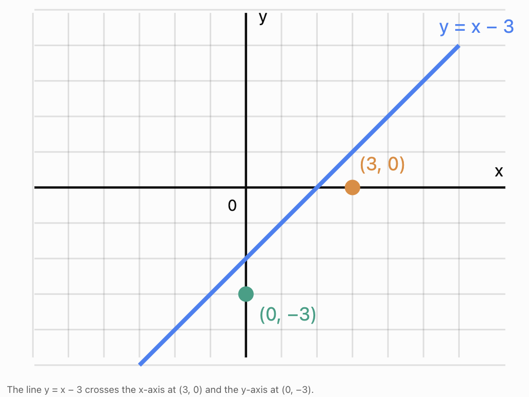
The orange point represents the x-intercept.
The green point represents the y-intercept.
Both intercepts can be found directly from the equation.
Understanding x-Intercepts
An x-intercept is a point where a graph meets the x-axis.
At an x-intercept:
y = 0
For a function written as:
y = f(x)
we find x-intercepts by solving:
f(x) = 0
The resulting x-values are also called the zeros or roots of the function.
Worked Example: Finding an x-intercept
Consider:
y = 3x − 12
Set y = 0:
0 = 3x − 12
Add 12:
12 = 3x
Divide by 3:
x = 4
Therefore, the x-intercept is:
(4, 0)
Verification
Substitute x = 4 into the original equation:
y = 3(4) − 12
y = 12 − 12
y = 0
The point lies on the x-axis, so the answer is correct.
Understanding y-Intercepts
A y-intercept is a point where a graph meets the y-axis.
At a y-intercept:
x = 0
To find the y-intercept, substitute x = 0 into the equation.
Worked Example: Finding a y-intercept
Consider:
y = 3x − 12
Substitute x = 0:
y = 3(0) − 12
y = −12
Therefore, the y-intercept is:
(0, −12)
Comparing the two intercepts
For:
y = 3x − 12
-
x-intercept: (4, 0).
-
y-intercept: (0, −12).
These points can be plotted and connected to sketch the straight line.
Intercepts of Linear Functions
A linear function has the general form:
y = mx + c
where:
-
m is the gradient.
-
c is the y-intercept value.
Finding the y-intercept
Set x = 0:
y = m(0) + c
y = c
Therefore:
y-intercept = (0, c)
Finding the x-intercept
Set y = 0:
0 = mx + c
mx = −c
If m ≠ 0:
x = −c/m
Therefore:
x-intercept = (−c/m, 0)
These formulas are useful when analyzing straight-line graphs.
Worked Example
Find both intercepts of:
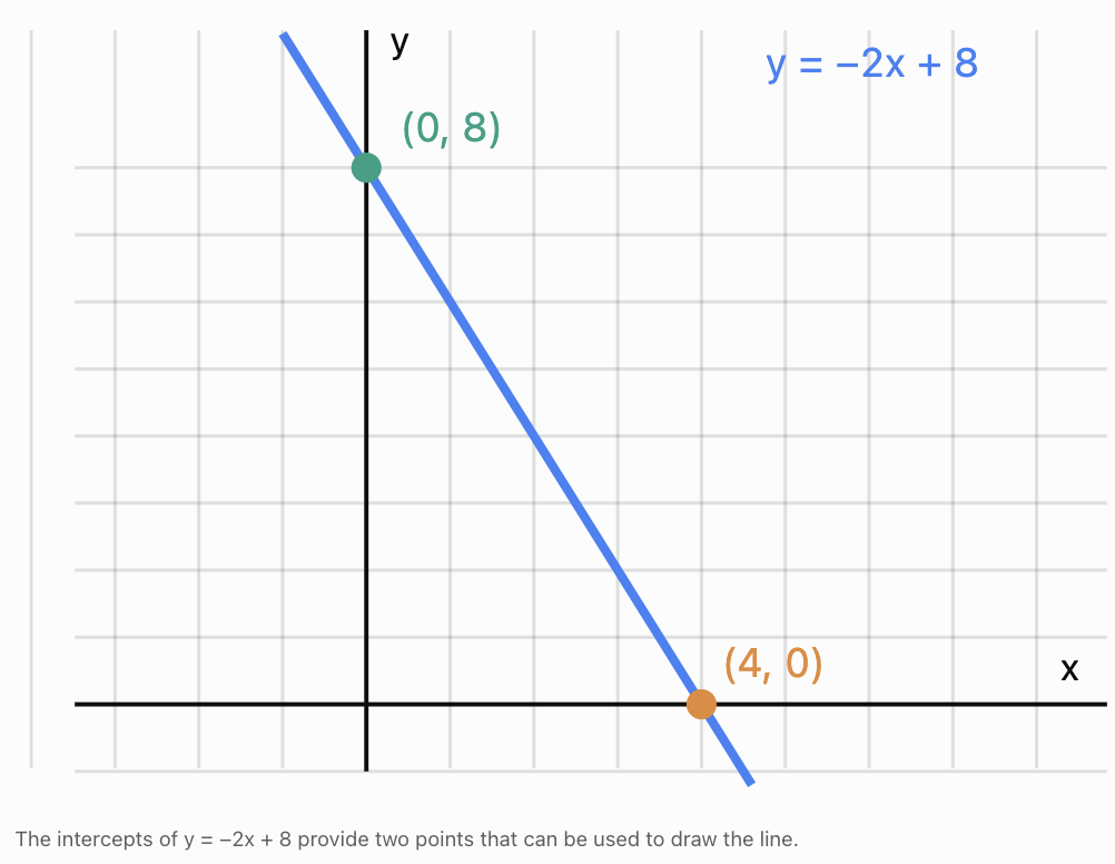
y = −2x + 8
x-intercept
Set y = 0:
0 = −2x + 8
2x = 8
x = 4
x-intercept: (4, 0)
y-intercept
Set x = 0:
y = −2(0) + 8
y = 8
y-intercept: (0, 8)
Using Intercepts to Sketch Linear Graphs
A straight line can be drawn using any two distinct points.
If a line has different x- and y-intercepts, these provide two convenient points.
Worked Example
Sketch:
y = 4x − 8
Find the x-intercept:
0 = 4x − 8
x = 2
Point: (2, 0)
Find the y-intercept:
x = 0
y = −8
Point: (0, −8)
Plot the two points and draw a straight line through them.
Special case: A line through the origin
Consider:
y = 3x
The x-intercept and y-intercept are both:
(0, 0)
These are not two distinct points.
To sketch the line, choose an additional point.
For example, when x = 1:
y = 3
So the line also passes through (1, 3).
Horizontal and vertical lines
The horizontal line y = 4 has a y-intercept at (0, 4), but no x-intercept.
The vertical line x = 3 has an x-intercept at (3, 0), but no y-intercept.
The horizontal line y = 0 lies along the x-axis, so every point on it is an x-intercept.
The vertical line x = 0 lies along the y-axis, so every point on it is a y-intercept.
These special cases remind us that not every graph has exactly one intercept of each type.
Intercepts of Quadratic Functions
Quadratic functions have the general form:
y = ax² + bx + c
where a ≠ 0.
Their graphs are parabolas.
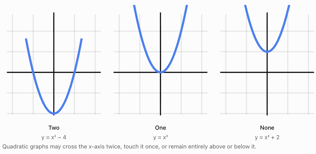
A parabola may have:
-
Two distinct x-intercepts.
-
Exactly one x-intercept, where it touches the x-axis.
-
No x-intercepts.
A quadratic function always has one y-intercept.
Finding the y-intercept
Set x = 0:
y = a(0)² + b(0) + c
y = c
Therefore:
y-intercept = (0, c)
Worked Example: Two x-intercepts
Consider:
y = x² − 5x + 6
Set y = 0:
0 = x² − 5x + 6
Factor:
0 = (x − 2)(x − 3)
Therefore:
x − 2 = 0 or x − 3 = 0
x = 2 or x = 3
The x-intercepts are:
(2, 0) and (3, 0)
To find the y-intercept, substitute x = 0:
y = 0² − 5(0) + 6
y = 6
y-intercept = (0, 6)
Worked Example: One x-intercept
Consider:
y = (x − 4)²
Set y = 0:
0 = (x − 4)²
x = 4
The parabola touches the x-axis at:
(4, 0)
This is a repeated root.
The graph does not cross the x-axis at this point; it touches the axis and turns around.
Worked Example: No x-intercepts
Consider:
y = x² + 3
Set y = 0:
0 = x² + 3
x² = −3
There are no real solutions because the square of a real number cannot be negative.
Therefore, the graph has no x-intercepts.
Its y-intercept is (0, 3).
The Discriminant and x-Intercepts
For a quadratic equation:
ax² + bx + c = 0
the discriminant is:
D = b² − 4ac
The discriminant tells us how many distinct real roots the quadratic has.
|
Discriminant |
Number of x-intercepts |
|---|---|
|
D > 0 |
Two distinct x-intercepts |
|
D = 0 |
One x-intercept |
|
D < 0 |
No x-intercepts |
Worked Example
Consider:
y = 2x² − 4x + 5
Identify:
a = 2, b = −4, c = 5
Calculate:
D = (−4)² − 4(2)(5)
D = 16 − 40
D = −24
Since D < 0, the graph has no x-intercepts.
Its y-intercept is:
(0, 5)
Intercepts of Other Function Families
The same intercept rules apply to other functions, although the algebraic methods may differ.
Absolute value functions
Consider:
y = |x − 3| − 2
For x-intercepts:
0 = |x − 3| − 2
|x − 3| = 2
Therefore:
x − 3 = 2 or x − 3 = −2
x = 5 or x = 1
x-intercepts:
(1, 0) and (5, 0)
For the y-intercept:
y = |0 − 3| − 2 = 1
(0, 1)
Square root functions
Consider:
y = √(x + 1) − 2
For the x-intercept:
0 = √(x + 1) − 2
√(x + 1) = 2
x + 1 = 4
x = 3
x-intercept = (3, 0)
For the y-intercept:
y = √1 − 2 = −1
y-intercept = (0, −1)
Exponential functions
Consider:
y = 2ˣ − 4
For the x-intercept:
0 = 2ˣ − 4
2ˣ = 4
x = 2
x-intercept = (2, 0)
For the y-intercept:
y = 2⁰ − 4
y = 1 − 4 = −3
y-intercept = (0, −3)
Notice that y = 2ˣ has no x-intercept because 2ˣ is always positive. Translating it downward by 4 creates an x-intercept.
Rational functions
Consider:
y = (x − 2)/(x + 3)
For the x-intercept, set the numerator equal to zero, provided the denominator is not zero:
x − 2 = 0
x = 2
x-intercept = (2, 0)
For the y-intercept, substitute x = 0:
y = −2/3
y-intercept = (0, −2/3)
The function is undefined at x = −3, so this value cannot be an intercept.
Estimating Intercepts from Graphs
Sometimes a graph is available but its equation is unknown.
In these situations, intercepts can be estimated by reading the coordinate axes.
Steps for estimating an x-intercept
-
Locate the point where the graph meets the x-axis.
-
Read its approximate x-coordinate.
-
Write the point in the form (x, 0).
-
Include an approximation sign if the value is not exact.
Steps for estimating a y-intercept
-
Locate the point where the graph meets the y-axis.
-
Read its approximate y-coordinate.
-
Write the point in the form (0, y).
-
Check the graph's scale carefully.
Worked Example
Suppose a curve crosses the x-axis slightly to the right of x = 1.5 and again near x = 4.2.
Its estimated x-intercepts might be:
(1.6, 0) and (4.2, 0)
If it crosses the y-axis near y = 7:
Estimated y-intercept = (0, 7)
These estimates should not be treated as exact values unless supported by an equation or precise data.
Estimating with an interactive graph
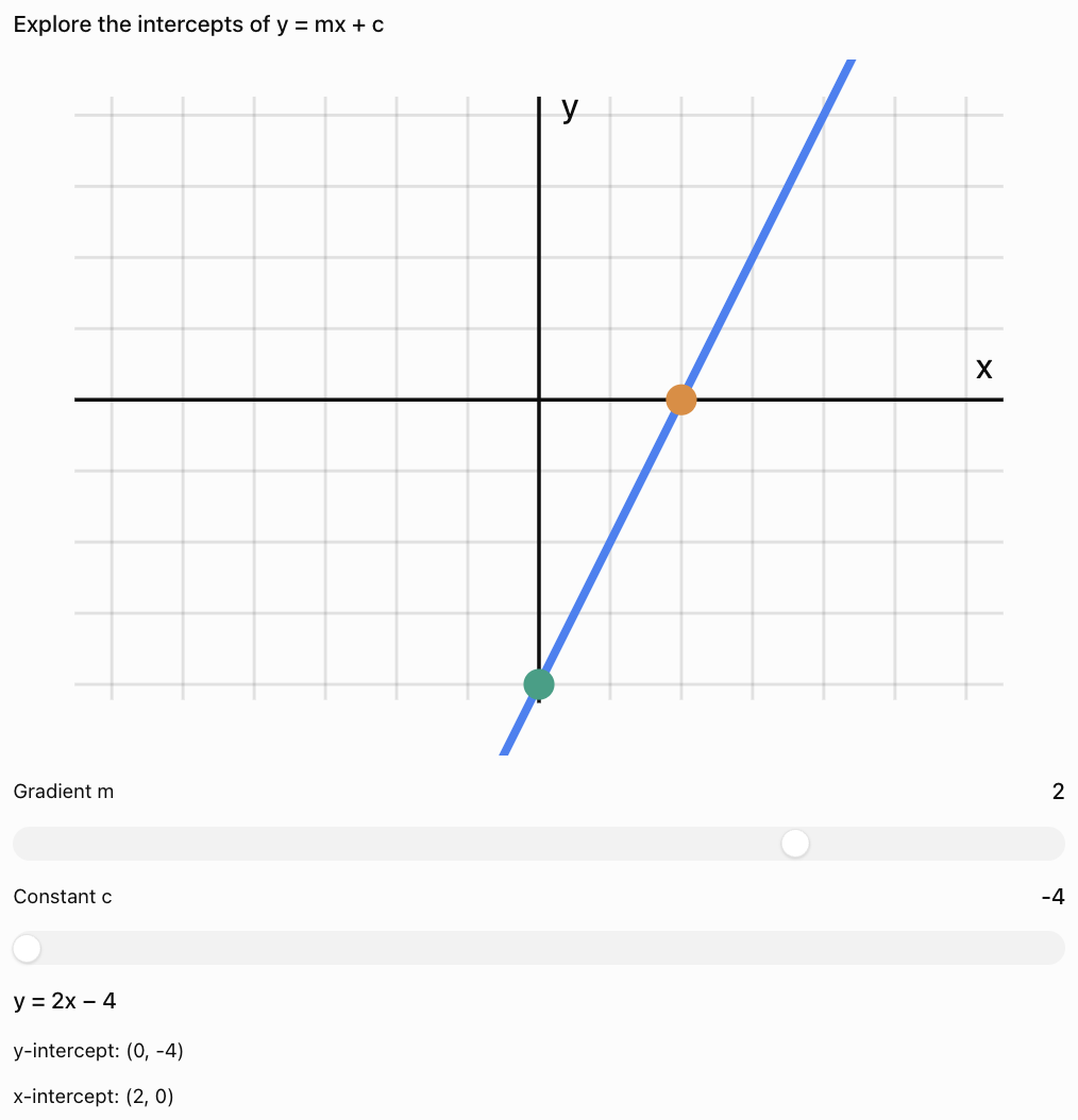
For classroom notes, the essential rules and calculations remain in the ordinary text above; the graph is an optional exploration.
Interpreting Intercepts in Real-World Situations
Intercepts become especially meaningful when a graph represents a real quantity.
Their interpretation depends on the variables, units, and context.
Application: Business break-even points
Suppose a company's profit is modeled by:
P(x) = 25x − 1000
where:
-
x = number of products sold.
-
P(x) = profit in dollars.
Finding the y-intercept
Set x = 0:
P(0) = 25(0) − 1000
P(0) = −1000
The y-intercept is:
(0, −1000)
This means the company has a loss of $1,000 when no products are sold.
Finding the x-intercept
Set P(x) = 0:
0 = 25x − 1000
25x = 1000
x = 40
The x-intercept is:
(40, 0)
This is the break-even point.
The company must sell 40 products to reach zero profit under this model.
For fewer than 40 products, the company makes a loss. For more than 40 products, it makes a profit.
Application: Height and Time
Suppose the height of a ball above the ground is:
h(t) = −5t² + 20t + 5
where:
-
h is height in metres.
-
t is time in seconds.
Finding the y-intercept
Set t = 0:
h(0) = 5
The intercept is:
(0, 5)
The ball starts 5 m above the ground.
Finding the x-intercepts
Set h(t) = 0:
0 = −5t² + 20t + 5
Divide by −5:
t² − 4t − 1 = 0
Using the quadratic formula:
t = 2 ± √5
Approximately:
t = −0.24 or t = 4.24
Mathematically, the graph has two x-intercepts.
However, if the model applies only from the moment the ball is released, t ≥ 0, the negative solution is outside the physical domain.
Therefore, the meaningful intercept is:
(4.24, 0), approximately
The ball reaches the ground after approximately 4.24 seconds.
This demonstrates why intercepts must be interpreted in context.
Application: Temperature
Suppose the temperature of a cooling substance is modeled by:
T(t) = 60 − 4t
where:
-
T is temperature in °C.
-
t is time in minutes.
y-intercept
T(0) = 60
The y-intercept is (0, 60).
This represents the initial temperature of 60°C.
x-intercept
Set T = 0:
0 = 60 − 4t
4t = 60
t = 15
The x-intercept is (15, 0).
This represents the time when the modeled temperature reaches 0°C.
The model is only appropriate over a time interval where its assumptions remain reasonable. It does not imply that the substance continues cooling linearly indefinitely.
Application: Water in a Tank
A tank contains 500 litres of water and drains at a constant rate of 20 litres per minute.
The volume is modeled by:
V(t) = 500 − 20t
where:
-
V = volume in litres.
-
t = time in minutes.
The y-intercept is:
(0, 500)
This represents the initial volume.
For the x-intercept:
0 = 500 − 20t
20t = 500
t = 25
x-intercept = (25, 0)
The tank becomes empty after 25 minutes.
The practical domain is:
0 ≤ t ≤ 25
The practical range is:
0 ≤ V ≤ 500
Comparing Intercepts of Different Functions
Intercepts provide a convenient way to compare mathematical models.
Consider three linear functions:
A: y = 2x + 4
B: y = 2x − 6
C: y = −x + 4
Calculate the intercepts
|
Function |
x-intercept |
y-intercept |
|---|---|---|
|
A: y = 2x + 4 |
(−2, 0) |
(0, 4) |
|
B: y = 2x − 6 |
(3, 0) |
(0, −6) |
|
C: y = −x + 4 |
(4, 0) |
(0, 4) |
Compare A and B
Both lines have gradient 2.
Therefore, they are parallel.
Their y-intercepts differ by 10 units.
Graph B is a vertical translation of Graph A downward by 10 units.
Their x-intercepts are also different.
Compare A and C
Both lines have the same y-intercept:
(0, 4)
However, their gradients are different.
Graph A increases from left to right, while Graph C decreases.
The two lines intersect at (0, 4).
Important conclusion
Two functions can share an x-intercept or y-intercept without having the same shape, gradient, or overall behaviour.
Intercepts are useful comparison points, but they do not describe an entire graph.
How Transformations Affect Intercepts
Graph transformations often change the intercepts of functions.
Vertical translation
Consider:
y = x² − 4
Its x-intercepts are:
(−2, 0) and (2, 0)
Its y-intercept is:
(0, −4)
Translate the graph upward by 4:
y = x²
The x-intercepts combine into one:
(0, 0)
The y-intercept becomes:
(0, 0)
Reflection across the x-axis
Consider:
y = x² − 4
Reflect across the x-axis:
y = −x² + 4
The x-intercepts remain:
(−2, 0) and (2, 0)
The y-intercept changes from:
(0, −4) to (0, 4)
This happens because reflection across the x-axis preserves points on the x-axis but reverses the signs of other y-coordinates.
Reflection across the y-axis
Consider:
y = (x − 3)² − 1
The x-intercepts are:
(2, 0) and (4, 0)
Reflect across the y-axis:
y = (x + 3)² − 1
The x-intercepts become:
(−2, 0) and (−4, 0)
The y-intercept remains unchanged.
This is because points on the y-axis remain fixed during reflection across the y-axis.
When Intercepts Do Not Exist
Not every function has an x-intercept or a y-intercept.
For example:
y = 2ˣ
This function has a y-intercept at (0, 1), but no x-intercept because 2ˣ is always positive.
y = 1/x
This function has neither an x-intercept nor a y-intercept.
It never equals zero, and it is undefined at x = 0.
x = 5
This vertical line has an x-intercept at (5, 0), but no y-intercept.
These examples demonstrate why intercepts must be determined from the actual function rather than assumed.
Common Mistakes
Confusing x-intercepts and y-intercepts
For x-intercepts, set y = 0.
For y-intercepts, set x = 0.
Writing only the intercept value
An intercept is a point, so write coordinates such as (3, 0), not simply 3.
Assuming every graph has two intercepts
Some graphs have no x-intercepts, while others have multiple x-intercepts.
Confusing roots with y-intercepts
Roots or zeros of a function are the x-values where f(x) = 0.
Ignoring domain restrictions
An algebraic solution may lie outside the permitted domain of the function or the practical domain of a real-world model.
Assuming an x-intercept always represents a break-even point
This interpretation is appropriate for certain profit models, but not every function.
Reading graph scales incorrectly
Check whether each grid interval represents 1, 2, 5, 10, or another quantity.
Assuming an estimated intercept is exact
Use an approximation sign when reading a value from a graph.
Dividing by zero when using formulas
The formula x = −c/m for a straight line applies only when m ≠ 0.
Assuming a graph must cross an axis at an intercept
A graph can touch an axis without crossing it, as happens at the vertex of y = (x − 2)².
Key Terms
-
Intercept: A point where a graph meets a coordinate axis.
-
x-intercept: A point where the graph meets the x-axis and y = 0.
-
y-intercept: A point where the graph meets the y-axis and x = 0.
-
Root: An input value that makes a function equal zero.
-
Zero of a function: An x-value satisfying f(x) = 0.
-
Solution: A value satisfying an equation.
-
Coordinate: A number specifying a point's position on an axis.
-
Origin: The point (0, 0), where the coordinate axes intersect.
-
Gradient: The rate of change of a straight-line graph.
-
Linear function: A function whose graph is a straight line.
-
Quadratic function: A function containing a squared variable as its highest power.
-
Parabola: The U-shaped or inverted U-shaped graph of a quadratic function.
-
Discriminant: The expression b² − 4ac used to determine the number of real roots of a quadratic equation.
-
Break-even point: The point where revenue equals cost and profit is zero.
-
Initial value: The value of a quantity when the input is zero.
-
Domain: The set of permitted input values.
-
Range: The set of possible output values.
-
Graph estimation: Approximating values by reading a plotted graph.
Key Takeaways
-
An x-intercept occurs where y = 0.
-
A y-intercept occurs where x = 0.
-
To find x-intercepts, solve f(x) = 0.
-
To find the y-intercept, calculate f(0), provided zero is in the domain.
-
The x-intercepts of a function correspond to its real roots or zeros.
-
A linear function may have one x-intercept, no x-intercept, or infinitely many points on the x-axis.
-
A quadratic function can have zero, one, or two distinct x-intercepts.
-
The discriminant helps determine how many x-intercepts a quadratic has.
-
Intercepts can be estimated from graphs or calculated algebraically.
-
In real-world models, intercepts often represent starting values, break-even points, or times when a quantity reaches zero.
-
Domain restrictions determine which intercepts are meaningful.
-
Comparing intercepts helps us understand similarities and differences between functions.
Check Your Understanding
Recall and Understanding
1. Define an x-intercept and explain how to identify one on a graph.
2. Define a y-intercept and explain how to calculate it from an equation.
3. Explain the relationship between x-intercepts and the roots of a function.
4. Can a quadratic function have no x-intercepts? Explain using an example.
Application
5. Find both intercepts of y = 4x − 12.
6. Find both intercepts of y = −3x + 9.
7. Find all intercepts of y = x² − 7x + 12.
8. Determine the number of x-intercepts of y = 2x² + 4x + 5 using the discriminant.
9. Find the intercepts of y = |x − 4| − 3.
10. A tank contains 360 litres of water and drains at 15 litres per minute. Write a volume-time equation and interpret both intercepts.
Analysis and Challenge
11. A company's profit is modeled by P(x) = 40x − 1600. Find the break-even point and explain its meaning.
12. Find the intercepts of y = (x − 2)² − 9. Explain why the graph has two x-intercepts.
13. Compare the intercepts of y = 2x + 6 and y = 2x − 4. What do the intercepts tell you about the graphs?
14. A ball's height is modeled by h(t) = −5t² + 15t + 20. Find the initial height and determine when it reaches the ground.
15. A student claims that y = 3ˣ has an x-intercept at (0, 1). Explain the error and identify the correct intercept.
Answers to Check Your Understanding
1. An x-intercept is a point where a graph meets the x-axis. Its y-coordinate is zero. It can be identified by locating where the graph crosses or touches the x-axis.
2. A y-intercept is a point where a graph meets the y-axis. Substitute x = 0 into the equation to calculate it.
3. Roots or zeros are the x-values that make f(x) = 0. Each real root in the domain corresponds to an x-intercept (x, 0).
4. Yes. For example, y = x² + 4 has no x-intercepts because x² + 4 is always positive for real x.
5.
y = 4x − 12
x-intercept:
0 = 4x − 12
x = 3
(3, 0)
y-intercept:
x = 0
y = −12
(0, −12)
6.
y = −3x + 9
x-intercept:
0 = −3x + 9
x = 3
(3, 0)
y-intercept:
(0, 9)
7.
y = x² − 7x + 12
For x-intercepts:
0 = (x − 3)(x − 4)
x = 3 or x = 4
(3, 0) and (4, 0)
For the y-intercept:
x = 0
y = 12
(0, 12)
8.
a = 2, b = 4, c = 5
D = b² − 4ac
D = 16 − 40
D = −24
Since D is negative, the graph has no x-intercepts.
9.
y = |x − 4| − 3
For x-intercepts:
0 = |x − 4| − 3
|x − 4| = 3
x − 4 = 3 or x − 4 = −3
x = 7 or x = 1
x-intercepts: (1, 0) and (7, 0)
For the y-intercept:
y = |0 − 4| − 3 = 1
y-intercept: (0, 1)
10.
Volume equation:
V(t) = 360 − 15t
y-intercept:
(0, 360)
The tank initially contains 360 litres.
x-intercept:
0 = 360 − 15t
t = 24
(24, 0)
The tank becomes empty after 24 minutes.
11.
P(x) = 40x − 1600
Set P(x) = 0:
0 = 40x − 1600
40x = 1600
x = 40
Break-even point: (40, 0)
The company must sell 40 products to cover its costs under this model.
12.
y = (x − 2)² − 9
For x-intercepts:
0 = (x − 2)² − 9
(x − 2)² = 9
x − 2 = ±3
x = 5 or x = −1
x-intercepts: (−1, 0) and (5, 0)
For the y-intercept:
y = (0 − 2)² − 9
y = −5
y-intercept: (0, −5)
The parabola opens upward and its vertex (2, −9) is below the x-axis, so it crosses the x-axis at two points.
13.
First function:
y = 2x + 6
x-intercept: (−3, 0)
y-intercept: (0, 6)
Second function:
y = 2x − 4
x-intercept: (2, 0)
y-intercept: (0, −4)
Both lines have gradient 2, so they are parallel.
The second graph is a vertical translation of the first downward by 10 units.
14.
h(t) = −5t² + 15t + 20
Initial height:
h(0) = 20
Initial height = 20 m
For the landing time:
0 = −5t² + 15t + 20
Divide by −5:
0 = t² − 3t − 4
Factor:
0 = (t − 4)(t + 1)
t = 4 or t = −1
The physically meaningful time is:
t = 4 seconds
15.
The student has confused the x-intercept with the y-intercept.
For y = 3ˣ:
At x = 0:
y = 3⁰ = 1
Therefore:
y-intercept = (0, 1)
Since 3ˣ is always positive for real x, it never equals zero.
Therefore, the function has no x-intercept.
Final Summary
Intercepts are essential features of graphs because they show where mathematical relationships meet the coordinate axes.
The two most important rules are:
x-intercepts: Set y = 0 and solve for x.
y-intercepts: Set x = 0 and solve for y.
By calculating, estimating, interpreting, and comparing intercepts, we can understand important characteristics of functions and connect mathematical graphs to real-world situations.
Intercepts provide a foundation for solving equations, sketching graphs, analyzing functions, and building mathematical models.
2. Increasing and Decreasing Functions
Learning outcomes
- I can identify increasing intervals.
- I can identify decreasing intervals.
- I can compare function behavior.
- I can interpret changes in graphs.
- I can describe function trends.
Introduction
Graphs show more than the relationship between two variables. They also reveal how a quantity changes as its input increases.
For example, imagine tracking the height of a ball thrown into the air.
-
At first, the ball moves upward, so its height increases.
-
At its highest point, its height stops increasing.
-
As the ball falls, its height decreases.
These changes can be described mathematically using increasing and decreasing functions.
Understanding where a function increases or decreases allows us to identify trends, compare graphs, locate maximum and minimum values, and interpret real-world data.
This is useful in many subjects:
-
Physics: Describing changes in height, speed, and energy.
-
Biology: Studying population growth and decline.
-
Economics: Analysing changes in profit, revenue, and costs.
-
Chemistry: Investigating how concentrations change during reactions.
-
Environmental science: Interpreting changes in temperature and other measurements.
What Is an Increasing Function?
A function is increasing over an interval when its output increases as its input increases.
In simple terms:
As x increases, y increases.
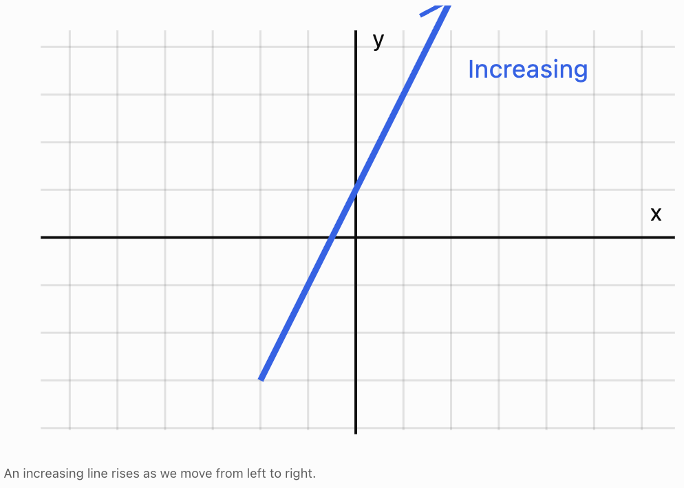
Imagine moving from left to right along a graph. If the graph rises, the function is increasing.
Example: A linear function
Consider:
y = 2x + 1
Calculate some values:
|
x |
y |
|---|---|
|
−2 |
−3 |
|
−1 |
−1 |
|
0 |
1 |
|
1 |
3 |
|
2 |
5 |
As x increases from −2 to 2, y increases from −3 to 5.
Therefore, the function is increasing over its entire domain.
Mathematical definition
A function f is strictly increasing on an interval if, whenever x₁ < x₂ in that interval:
f(x₁) < f(x₂)
This means a larger input always gives a larger output.
For example:
If x₁ = 1 and x₂ = 3, then for f(x) = 2x + 1:
f(1) = 3
f(3) = 7
Since 1 < 3 and 3 < 7, these values are consistent with an increasing function.
One pair of values alone does not prove that a function is increasing over an entire interval, but it helps illustrate the idea.
What Is a Decreasing Function?
A function is decreasing over an interval when its output decreases as its input increases.
In simple terms:
As x increases, y decreases.
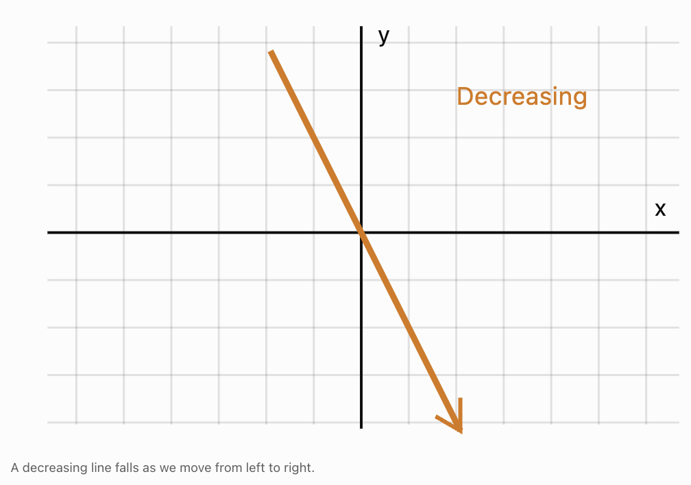
When moving from left to right along a graph, a decreasing function falls.
Example: A linear function
Consider:
y = −3x + 4
|
x |
y |
|---|---|
|
−2 |
10 |
|
−1 |
7 |
|
0 |
4 |
|
1 |
1 |
|
2 |
−2 |
As x increases, y decreases.
Therefore, the function is decreasing over its entire domain.
Mathematical definition
A function f is strictly decreasing on an interval if, whenever x₁ < x₂:
f(x₁) > f(x₂)
This means a larger input always gives a smaller output.
Constant Functions
Not every function is increasing or decreasing.
Consider:
y = 5
Regardless of the value of x, the output remains 5.
|
x |
y |
|---|---|
|
−2 |
5 |
|
−1 |
5 |
|
0 |
5 |
|
1 |
5 |
|
2 |
5 |
The graph is a horizontal line.
It is constant over its entire domain.
In strict terminology, a constant function is neither strictly increasing nor strictly decreasing.
Some textbooks also use non-decreasing and non-increasing:
-
Non-decreasing means outputs never go down as x increases.
-
Non-increasing means outputs never go up as x increases.
Under these broader definitions, a constant function is both non-decreasing and non-increasing.
For these notes, increasing and decreasing will generally mean strictly increasing and decreasing unless stated otherwise.
Understanding Intervals
Many functions are not increasing or decreasing everywhere.
Instead, their behaviour changes over different parts of their domains.
An interval is a continuous section of the x-axis.
For example:
−3 < x < 2
describes all x-values between −3 and 2.
In interval notation, this is written:
(−3, 2)
The parentheses indicate that the endpoints are not included.
Common interval notation
|
Notation |
Meaning |
|---|---|
|
(a, b) |
Between a and b, excluding both endpoints |
|
[a, b] |
Between a and b, including both endpoints |
|
(−∞, a) |
All values less than a |
|
(a, ∞) |
All values greater than a |
|
(−∞, ∞) |
All real numbers |
Infinity always uses parentheses because it is not a real endpoint.
Why interval notation matters
A function may increase over one interval and decrease over another.
We need a precise way to describe where each behaviour occurs.
Identifying Increasing and Decreasing Intervals from Graphs
To identify intervals:
-
Read the graph from left to right.
-
Identify sections where the graph rises.
-
Identify sections where the graph falls.
-
Locate any turning points.
-
Record the corresponding x-values using interval notation.
Worked Example: A quadratic function
Consider:
f(x) = x²
The graph is a U-shaped parabola with vertex at (0, 0).
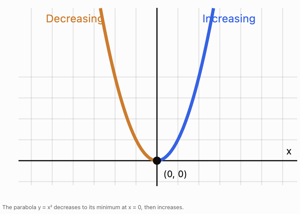
On the left side of the vertex, the graph falls as x increases.
On the right side, the graph rises.
Therefore:
Decreasing interval: (−∞, 0)
Increasing interval: (0, ∞)
The vertex at x = 0 is a turning point where the direction changes.
We usually use open intervals when reporting increasing and decreasing behaviour so that turning points clearly separate the intervals. For continuous functions, including the turning-point endpoint can also be mathematically valid when describing monotonicity on a closed or half-closed interval.
Increasing and Decreasing Quadratic Functions
The direction of a quadratic function depends on whether its parabola opens upward or downward.
The vertex is particularly important because it separates the increasing and decreasing intervals.
Upward-opening parabolas
Consider:
f(x) = (x − 3)² + 2
The vertex is:
(3, 2)
The graph opens upward, so it decreases until x = 3 and then increases.
-
Decreasing: (−∞, 3)
-
Increasing: (3, ∞)
-
Minimum value: 2
Downward-opening parabolas
Consider:
g(x) = −2(x + 1)² + 8
The vertex is:
(−1, 8)
The graph opens downward, so it increases until x = −1 and then decreases.
-
Increasing: (−∞, −1)
-
Decreasing: (−1, ∞)
-
Maximum value: 8
Comparing the two types
|
Feature |
Opens upward |
Opens downward |
|---|---|---|
|
Quadratic coefficient |
Positive |
Negative |
|
Left of vertex |
Decreasing |
Increasing |
|
Right of vertex |
Increasing |
Decreasing |
|
Vertex represents |
Minimum |
Maximum |
Worked Example: Finding intervals from standard form
Consider:
f(x) = 2x² − 8x + 5
The x-coordinate of the vertex is:
x = −b/(2a)
Here:
a = 2, b = −8
Substitute:
x = −(−8)/(2 × 2)
x = 8/4
x = 2
Because a is positive, the parabola opens upward.
Therefore:
Decreasing: (−∞, 2)
Increasing: (2, ∞)
To calculate the minimum:
f(2) = 2(2)² − 8(2) + 5
f(2) = 8 − 16 + 5
f(2) = −3
The minimum occurs at:
(2, −3)
Increasing and Decreasing Linear Functions
For a linear function:
y = mx + c
the gradient m determines its behaviour.
-
If m > 0, the function is increasing.
-
If m < 0, the function is decreasing.
-
If m = 0, the function is constant.
Worked Example
Compare:
A: y = 4x + 2
B: y = −2x + 7
C: y = 5
Function A has gradient 4, so it is increasing everywhere.
Function B has gradient −2, so it is decreasing everywhere.
Function C has gradient 0, so it is constant everywhere.
Both A and B have domains consisting of all real numbers.
Therefore:
-
A is increasing on (−∞, ∞).
-
B is decreasing on (−∞, ∞).
-
C is constant on (−∞, ∞).
Comparing rates of change
Consider:
f(x) = 2x + 1
g(x) = 5x + 1
Both functions are increasing.
However, g(x) increases more rapidly because its gradient is larger.
For each increase of 1 in x:
-
f(x) increases by 2.
-
g(x) increases by 5.
A function can therefore be increasing without increasing at the same rate as another function.
Increasing and Decreasing Absolute Value Functions
Consider the parent function:
f(x) = |x|
Its graph has a V shape.
The vertex is (0, 0).
To the left of the vertex, the function decreases.
To the right, it increases.
Therefore:
-
Decreasing: (−∞, 0)
-
Increasing: (0, ∞)
Worked Example: Transformed absolute value function
Consider:
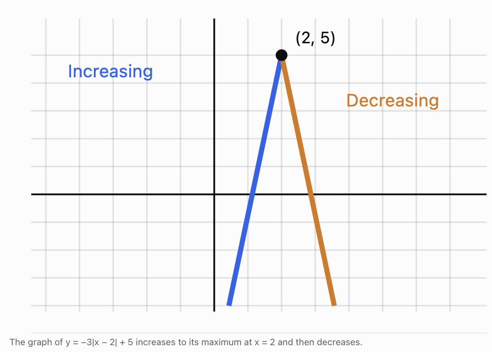
g(x) = −3|x − 2| + 5
The vertex is:
(2, 5)
The negative coefficient reflects the graph across the x-axis.
It becomes an upside-down V.
Therefore:
Increasing: (−∞, 2)
Decreasing: (2, ∞)
The function has a maximum value of 5.
Increasing and Decreasing Exponential Functions
Exponential functions are often used to model growth and decay.
Consider:
f(x) = 2ˣ
As x increases, the output increases.
For example:
|
x |
2ˣ |
|---|---|
|
−2 |
0.25 |
|
−1 |
0.5 |
|
0 |
1 |
|
1 |
2 |
|
2 |
4 |
The function is increasing on:
(−∞, ∞)
Now consider:
g(x) = (1/2)ˣ
|
x |
(1/2)ˣ |
|---|---|
|
−2 |
4 |
|
−1 |
2 |
|
0 |
1 |
|
1 |
0.5 |
|
2 |
0.25 |
The function is decreasing on:
(−∞, ∞)
General rule
For:
y = bˣ
where b > 0 and b ≠ 1:
-
If b > 1, the function is increasing.
-
If 0 < b < 1, the function is decreasing.
A vertical reflection can reverse these trends.
For example:
y = −2ˣ
is decreasing because it is the reflection of an increasing exponential function across the x-axis.
Functions with Several Increasing and Decreasing Intervals
Some functions change direction more than once.
Consider:
f(x) = x³ − 3x
This cubic function has two turning points.
The turning points are:
-
A local maximum at (−1, 2).
-
A local minimum at (1, −2).
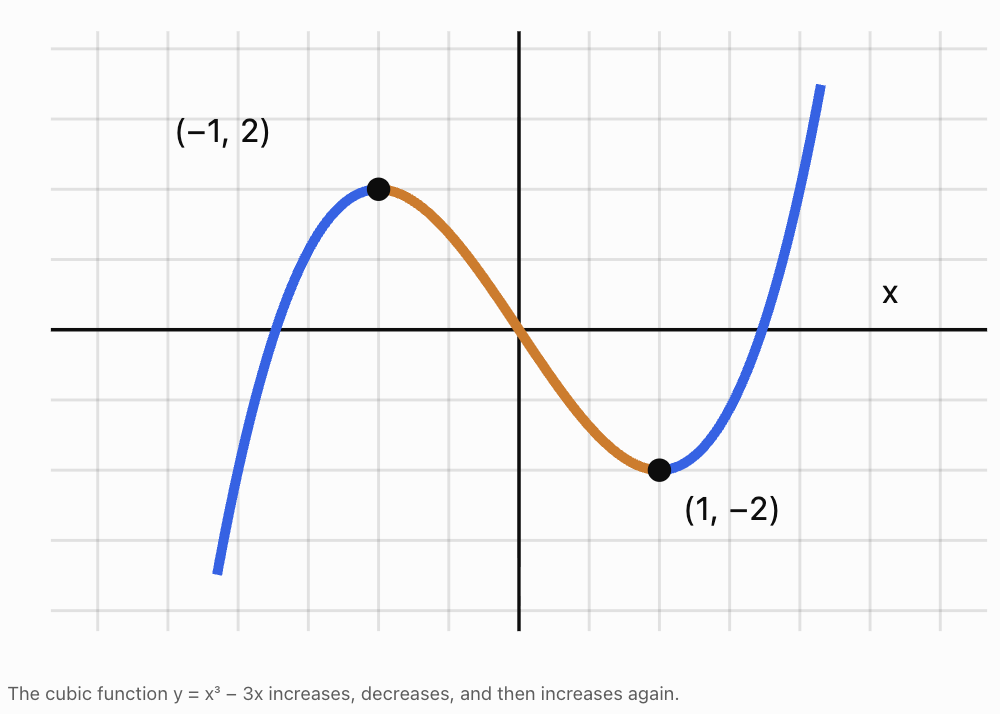
Read the graph from left to right:
-
It rises until x = −1.
-
It falls between x = −1 and x = 1.
-
It rises again after x = 1.
Therefore:
Increasing: (−∞, −1) and (1, ∞)
Decreasing: (−1, 1)
A function can have several separate increasing intervals.
We list these intervals individually rather than combining them into one interval that includes decreasing behaviour.
Using Tables to Identify Trends
Sometimes we have a table rather than a graph.
Consider:
|
Time |
Temperature (°C) |
|---|---|
|
8 |
18 |
|
9 |
21 |
|
10 |
24 |
|
11 |
26 |
|
12 |
26 |
|
13 |
25 |
|
14 |
23 |
From the table:
-
Temperature rises from 8:00 to 11:00.
-
Temperature stays unchanged between 11:00 and 12:00.
-
Temperature falls from 12:00 to 14:00.
We can describe the observed trend as:
Increasing: 8:00–11:00
Constant: 11:00–12:00
Decreasing: 12:00–14:00
However, a table only shows measured values.
Without additional information, we cannot be certain that the temperature increased continuously between every pair of measurements.
A graph or mathematical model can help estimate the behaviour between observations.
Comparing Function Behaviour
When comparing two functions, we can investigate more than whether they are increasing or decreasing.
We can also compare how rapidly their outputs change.
Example: Two increasing linear functions
Consider:
f(x) = 2x + 1
g(x) = 5x − 3
Both functions are increasing over all real numbers.
However, their gradients differ.
-
f(x) increases by 2 units for every increase of 1 in x.
-
g(x) increases by 5 units for every increase of 1 in x.
Therefore, g(x) increases more rapidly.
Example: Linear versus exponential growth
Consider:
f(x) = 2x + 1
g(x) = 2ˣ
Both functions are increasing.
However, their rates of change behave differently.
|
x |
f(x) = 2x + 1 |
g(x) = 2ˣ |
|---|---|---|
|
0 |
1 |
1 |
|
1 |
3 |
2 |
|
2 |
5 |
4 |
|
3 |
7 |
8 |
|
4 |
9 |
16 |
|
5 |
11 |
32 |
The linear function increases by a constant amount.
The exponential function increases by a constant percentage, so its absolute increases become larger.
At first, the linear function is larger.
Later, the exponential function becomes much larger.
Two functions can both be increasing while having very different long-term behaviour.
Average Rate of Change
The average rate of change measures how much a function's output changes per unit increase in its input over an interval.
For a function f(x), between x = a and x = b:
Average rate of change = [f(b) − f(a)]/(b − a)
where a ≠ b.
This is the gradient of the secant line joining the two points on the graph.
Worked Example
Consider:
f(x) = x²
Find the average rate of change between x = 1 and x = 3.
First calculate:
f(1) = 1
f(3) = 9
Then:
Average rate of change = (9 − 1)/(3 − 1)
= 8/2
= 4
Over this interval, the output increases by an average of 4 units for each increase of 1 in x.
Positive and negative average rates
-
A positive average rate means the output at the end is greater than at the start.
-
A negative average rate means the output at the end is smaller than at the start.
-
A zero average rate means the endpoint outputs are equal.
However, a positive average rate does not prove that the function increases throughout the interval.
For example, a graph could rise, fall, and then rise again while still ending higher than it started.
Local Maximum and Minimum Points
An increasing function may eventually stop increasing and begin decreasing.
The point where this happens is often a local maximum.
Similarly, a function may stop decreasing and begin increasing.
This point is often a local minimum.
Local maximum
A local maximum occurs when a function has a value greater than or equal to nearby function values.
For example:
f(x) = −(x − 2)² + 5
The graph increases until x = 2, then decreases.
The vertex (2, 5) is a local maximum.
It is also the absolute maximum of this function.
Local minimum
A local minimum occurs when a function has a value less than or equal to nearby function values.
For example:
g(x) = (x + 3)² − 4
The graph decreases until x = −3, then increases.
The vertex (−3, −4) is a local minimum.
It is also the absolute minimum.
Local versus absolute extrema
A local maximum is higher than nearby values.
An absolute maximum is the greatest value over the entire domain being considered.
Similarly, a local minimum is lower than nearby values, while an absolute minimum is the smallest value over the domain.
A function can have several local maxima and minima without having an absolute maximum or minimum.
How Transformations Affect Increasing and Decreasing Intervals
Graph transformations can change the intervals over which a function increases or decreases.
Vertical translations
Consider:
f(x) = x²
g(x) = x² + 5
Both functions:
-
Decrease on (−∞, 0).
-
Increase on (0, ∞).
A vertical translation does not change where the function increases or decreases.
Horizontal translations
Consider:
f(x) = x²
g(x) = (x − 4)²
For f(x):
-
Decreasing: (−∞, 0)
-
Increasing: (0, ∞)
For g(x):
-
Decreasing: (−∞, 4)
-
Increasing: (4, ∞)
The horizontal translation shifts the turning point and therefore shifts the interval boundaries.
Reflection across the x-axis
Consider:
f(x) = x²
g(x) = −x²
For f(x):
-
Decreasing: (−∞, 0)
-
Increasing: (0, ∞)
For g(x):
-
Increasing: (−∞, 0)
-
Decreasing: (0, ∞)
A reflection across the x-axis reverses increasing and decreasing behaviour.
Vertical stretches and compressions
Multiplying a function by a positive number does not change its increasing or decreasing intervals.
For example:
f(x) = x²
g(x) = 5x²
Both decrease for x < 0 and increase for x > 0.
The graph becomes narrower, but the direction of change remains the same.
Real-World Application: Projectile Motion
A ball is thrown upward from a platform.
Its height is modeled by:
h(t) = −5t² + 20t + 5
where:
-
h is height in metres.
-
t is time in seconds.
Step 1: Find the turning point
The vertex occurs at:
t = −b/(2a)
Here:
a = −5, b = 20
t = −20/[2(−5)]
t = 2
Step 2: Calculate the maximum height
h(2) = −5(2)² + 20(2) + 5
h(2) = −20 + 40 + 5
h(2) = 25
Maximum height:
25 m
Step 3: Identify the intervals
The ball rises from t = 0 to t = 2.
Therefore, height is increasing on:
(0, 2)
The ball then falls until it reaches the ground.
Solve:
−5t² + 20t + 5 = 0
t = 2 + √5 ≈ 4.24 s
Therefore, over the physical flight:
Decreasing: (2, 4.24), approximately
Interpretation
The ball's height increases while it rises and decreases while it falls.
Notice that the ball is moving during both intervals.
A decreasing height does not mean the ball has stopped moving; it means its vertical position is becoming smaller.
Real-World Application: Population Changes
Suppose a population is modeled by:
P(t) = 500(1.06)ᵗ
where t is time in years.
Since the exponential base 1.06 is greater than 1, the function is increasing.
The population grows by 6% each year under the model.
Now consider:
Q(t) = 500(0.94)ᵗ
Because 0.94 is between 0 and 1, the function is decreasing.
The population declines by 6% each year.
Comparing the models
Both populations begin at 500.
However:
-
P(t) represents exponential growth.
-
Q(t) represents exponential decay.
The difference becomes greater over time.
These models could represent populations under different environmental conditions, although actual populations are affected by many factors.
Real-World Application: Business Profit
Suppose a business models profit using:
P(x) = −2(x − 30)² + 1800
where x represents hundreds of products sold.
The parabola opens downward.
Its vertex is:
(30, 1800)
Therefore, the maximum modeled profit is $1,800 when 3,000 products are sold.
Increasing interval
For x < 30, profit increases as sales increase.
Within the practical domain x ≥ 0:
Increasing: (0, 30)
Decreasing interval
For x > 30, profit decreases as sales increase.
Decreasing: (30, ∞)
The second interval describes the mathematical model, although real-world production constraints may restrict its domain.
Interpretation
Selling more products does not always increase profit under this model.
Beyond the optimal sales level, additional costs or pricing effects may reduce profitability.
Real-World Application: Temperature Trends
Consider a simplified temperature model:
T(t) = −0.5(t − 14)² + 30
where t represents the hour of the day.
The vertex is:
(14, 30)
The maximum modeled temperature is 30°C at 14:00, or 2:00 p.m.
The function:
-
Increases before 14:00.
-
Decreases after 14:00.
Over the interval 8 ≤ t ≤ 20:
Increasing: (8, 14)
Decreasing: (14, 20)
This model could represent a simplified daily temperature pattern.
Actual temperatures may fluctuate and do not necessarily follow a perfect parabola.
Describing Function Trends
When describing a graph, it is useful to go beyond simply stating that it increases or decreases.
Consider the following descriptions:
|
Trend |
Meaning |
|---|---|
|
Increasing steadily |
Output rises at a constant rate |
|
Increasing more rapidly |
Output rises at an increasing rate |
|
Increasing more slowly |
Output rises, but its rate of increase becomes smaller |
|
Decreasing steadily |
Output falls at a constant rate |
|
Decreasing more rapidly |
Output falls at an increasingly negative rate |
|
Decreasing more slowly |
Output falls, but the rate of decrease becomes smaller |
|
Constant |
Output remains unchanged |
|
Fluctuating |
Output alternates between increases and decreases |
Example: Comparing two increasing functions
Consider:
f(x) = x
g(x) = x², for x ≥ 0
Both functions are increasing.
However:
-
f(x) increases at a constant rate.
-
g(x) increases more rapidly as x becomes larger.
Example: Increasing at a decreasing rate
Consider:
h(x) = √x, for x ≥ 0
The function increases as x increases.
However, the graph becomes progressively flatter.
For example:
|
x |
√x |
|---|---|
|
0 |
0 |
|
1 |
1 |
|
4 |
2 |
|
9 |
3 |
|
16 |
4 |
The output increases by 1 each time, but increasingly large changes in x are required.
Therefore, the function is increasing at a decreasing rate.
This distinction is important when analysing growth trends.
A Step-by-Step Method for Analysing Function Behaviour
When given an unfamiliar graph, use the following approach.
Step 1: Identify the domain.
Determine which x-values are included.
Step 2: Read the graph from left to right.
Observe whether the graph rises, falls, or stays horizontal.
Step 3: Locate turning points.
Identify where the direction changes.
Step 4: Record interval boundaries.
Use the x-coordinates of turning points and domain endpoints.
Step 5: Write increasing and decreasing intervals.
Use interval notation.
Step 6: Identify maximum and minimum values.
Determine whether turning points represent local or absolute extrema.
Step 7: Describe the trend in context.
Explain what increasing or decreasing means for the quantities being measured.
Step 8: Compare rates of change when appropriate.
Determine whether the function changes steadily, more rapidly, or more slowly.
Common Mistakes
Reading a graph from right to left
Increasing and decreasing intervals are determined by moving from left to right, in the direction of increasing x.
Confusing positive values with increasing functions
A function can have positive outputs while decreasing.
For example, y = 10 − x is decreasing even when y is positive.
Confusing negative values with decreasing functions
A function can have negative outputs while increasing.
For example, y = x − 10 is increasing everywhere.
Using y-values instead of x-values in interval notation
Increasing and decreasing intervals are described using input values.
Ignoring turning points
A quadratic function may increase over one interval and decrease over another.
Assuming a steeper graph always means an increasing function
A steep downward line is decreasing.
Steepness and direction are different properties.
Confusing decreasing with decreasing more rapidly
A function can decrease while becoming flatter, meaning its rate of decrease is slowing.
Assuming a positive average rate proves a function is increasing throughout
Average rate of change only compares the endpoints.
Ignoring the practical domain
A mathematical model may be defined beyond the time or quantity relevant to the real situation.
Assuming a stationary point must be a maximum or minimum
For example, y = x³ has a horizontal tangent at x = 0 but continues increasing through that point.
Key Terms
-
Increasing function: A function whose outputs rise as inputs increase.
-
Decreasing function: A function whose outputs fall as inputs increase.
-
Strictly increasing: Larger inputs always produce larger outputs within an interval.
-
Strictly decreasing: Larger inputs always produce smaller outputs within an interval.
-
Constant function: A function whose output remains unchanged.
-
Interval: A continuous set of input values.
-
Interval notation: A method of representing sets of values using brackets or parentheses.
-
Turning point: A point where a graph changes from increasing to decreasing or vice versa.
-
Local maximum: A function value greater than or equal to nearby values.
-
Local minimum: A function value less than or equal to nearby values.
-
Absolute maximum: The greatest output over a specified domain.
-
Absolute minimum: The smallest output over a specified domain.
-
Gradient: The rate of change of a straight-line graph.
-
Average rate of change: The change in output divided by the change in input over an interval.
-
Monotonic function: A function that is consistently non-decreasing or non-increasing over an interval.
-
Exponential growth: Growth by a constant percentage over equal input intervals.
-
Exponential decay: Decline by a constant percentage over equal input intervals.
-
Trend: The general direction or pattern of change in a graph or dataset.
-
Domain: The set of permitted input values.
-
Range: The set of possible output values.
Key Takeaways
-
A function is increasing when its outputs rise as x increases.
-
A function is decreasing when its outputs fall as x increases.
-
Increasing and decreasing intervals are identified by reading graphs from left to right.
-
Intervals are written using x-values, not y-values.
-
Linear functions with positive gradients are increasing.
-
Linear functions with negative gradients are decreasing.
-
Upward-opening parabolas decrease before their vertex and increase afterward.
-
Downward-opening parabolas increase before their vertex and decrease afterward.
-
Functions may have several increasing and decreasing intervals.
-
A turning point often separates intervals with different behaviour.
-
Increasing functions do not necessarily increase at constant rates.
-
Average rate of change measures the overall change between two input values.
-
Graph transformations can change increasing and decreasing intervals.
-
Understanding trends helps interpret real-world situations and make predictions.
Check Your Understanding
Recall and Understanding
1. Define an increasing function.
2. Define a decreasing function.
3. Explain how to identify increasing intervals from a graph.
4. What is the difference between a decreasing function and a constant function?
Application
5. Determine whether y = 5x − 3 is increasing or decreasing. State the interval.
6. Determine whether y = −4x + 7 is increasing or decreasing. State the interval.
7. Find the increasing and decreasing intervals of y = x² − 6x + 5.
8. Find the increasing and decreasing intervals of y = −2(x + 4)² + 9.
9. Determine the increasing and decreasing intervals of y = |x − 5|.
10. Calculate the average rate of change of f(x) = x² between x = 2 and x = 5.
Analysis and Challenge
11. Compare the behaviour of f(x) = 3x + 1 and g(x) = 7x − 2.
12. A ball's height is modeled by h(t) = −5t² + 30t + 2. Determine when its height is increasing and when it is decreasing during its flight.
13. Determine the increasing and decreasing intervals of f(x) = x³ − 12x, given that its turning points occur at x = −2 and x = 2.
14. Explain why y = √x is increasing but its rate of increase becomes smaller as x increases.
15. A business models profit using P(x) = −3(x − 20)² + 1500, where x is the number of products sold. Identify the increasing and decreasing intervals for x ≥ 0 and interpret the maximum.
Answers to Check Your Understanding
1. An increasing function has outputs that rise as its inputs increase. For a strictly increasing function, x₁ < x₂ implies f(x₁) < f(x₂).
2. A decreasing function has outputs that fall as its inputs increase. For a strictly decreasing function, x₁ < x₂ implies f(x₁) > f(x₂).
3. Read the graph from left to right. Identify sections where the graph rises and record the corresponding x-values using interval notation.
4. A decreasing function has outputs that become smaller as x increases. A constant function has outputs that remain unchanged.
5.
y = 5x − 3
Gradient = 5.
Since the gradient is positive, the function is increasing on:
(−∞, ∞)
6.
y = −4x + 7
Gradient = −4.
Since the gradient is negative, the function is decreasing on:
(−∞, ∞)
7.
y = x² − 6x + 5
a = 1, b = −6
Vertex x-coordinate:
x = −b/(2a)
x = 6/2 = 3
The parabola opens upward.
Decreasing: (−∞, 3)
Increasing: (3, ∞)
8.
y = −2(x + 4)² + 9
Vertex x-coordinate:
x = −4
The parabola opens downward.
Increasing: (−∞, −4)
Decreasing: (−4, ∞)
9.
y = |x − 5|
Vertex:
(5, 0)
The graph is V-shaped.
Decreasing: (−∞, 5)
Increasing: (5, ∞)
10.
f(x) = x²
f(2) = 4
f(5) = 25
Average rate of change:
= (25 − 4)/(5 − 2)
= 21/3
= 7
11.
f(x) = 3x + 1
g(x) = 7x − 2
Both functions are increasing on (−∞, ∞) because both gradients are positive.
However, g(x) increases more rapidly because its gradient is 7, compared with 3 for f(x).
12.
h(t) = −5t² + 30t + 2
The vertex occurs at:
t = −30/[2(−5)]
t = 3
Therefore, height increases until t = 3 seconds.
To find the landing time:
0 = −5t² + 30t + 2
5t² − 30t − 2 = 0
Using the quadratic formula:
t = [30 ± √(900 + 40)]/10
t = [30 ± √940]/10
The positive solution is approximately:
t ≈ 6.07 s
Therefore, during the physical flight:
Increasing: (0, 3)
Decreasing: (3, 6.07), approximately
13.
f(x) = x³ − 12x
The turning points occur at x = −2 and x = 2.
The function increases before x = −2, decreases between the turning points, and increases after x = 2.
Increasing: (−∞, −2) and (2, ∞)
Decreasing: (−2, 2)
14.
For y = √x, larger x-values produce larger y-values.
However, the graph becomes flatter as x increases.
For example:
-
From x = 0 to x = 1, y increases by 1.
-
From x = 1 to x = 4, y increases by 1 over 3 x-units.
-
From x = 4 to x = 9, y increases by 1 over 5 x-units.
The same increase in y requires increasingly large changes in x.
Therefore, the function is increasing at a decreasing rate.
15.
P(x) = −3(x − 20)² + 1500
The vertex is:
(20, 1500)
Because the parabola opens downward, the vertex represents a maximum.
For the practical domain x ≥ 0:
Increasing: (0, 20)
Decreasing: (20, ∞)
The maximum modeled profit is:
$1,500 when 20 products are sold.
The model suggests that increasing sales improves profit until 20 products are sold, after which further increases in sales reduce profit.
Final Summary
Increasing and decreasing functions describe how outputs change as inputs increase.
By examining graphs from left to right, identifying turning points, and using interval notation, we can determine where functions rise, fall, or remain constant.
These ideas allow us to compare function behaviour, understand maximum and minimum values, interpret rates of change, and describe trends in real-world situations.
The key distinction is between the value of a function and the direction in which that value is changing.
3. Maximums and Minimums
Learning outcomes
- I can identify maximum values.
- I can identify minimum values.
- I can locate turning points.
- I can interpret extrema in context.
- I can compare maximums and minimums across functions.
Introduction
Many real-world situations involve finding the greatest or smallest possible value of a quantity.
For example:
-
What is the maximum height reached by a ball thrown into the air?
-
What is the minimum cost of producing a product?
-
At what point does a business earn its greatest profit?
-
What is the lowest temperature recorded during a day?
-
How can an engineer design a structure using the least amount of material?
These questions involve maximums and minimums, also known as extrema.
In mathematics, extrema are important features of functions because they help us understand the behaviour of graphs, identify turning points, compare different models, and solve optimisation problems.
A maximum is a greatest value, while a minimum is a smallest value. However, we must distinguish between values that are greatest or smallest over an entire domain and those that are greatest or smallest only compared with nearby values.
Understanding this distinction is essential when analysing functions.
What Is a Maximum Value?
A maximum value is the greatest output a function reaches over a specified domain or interval.
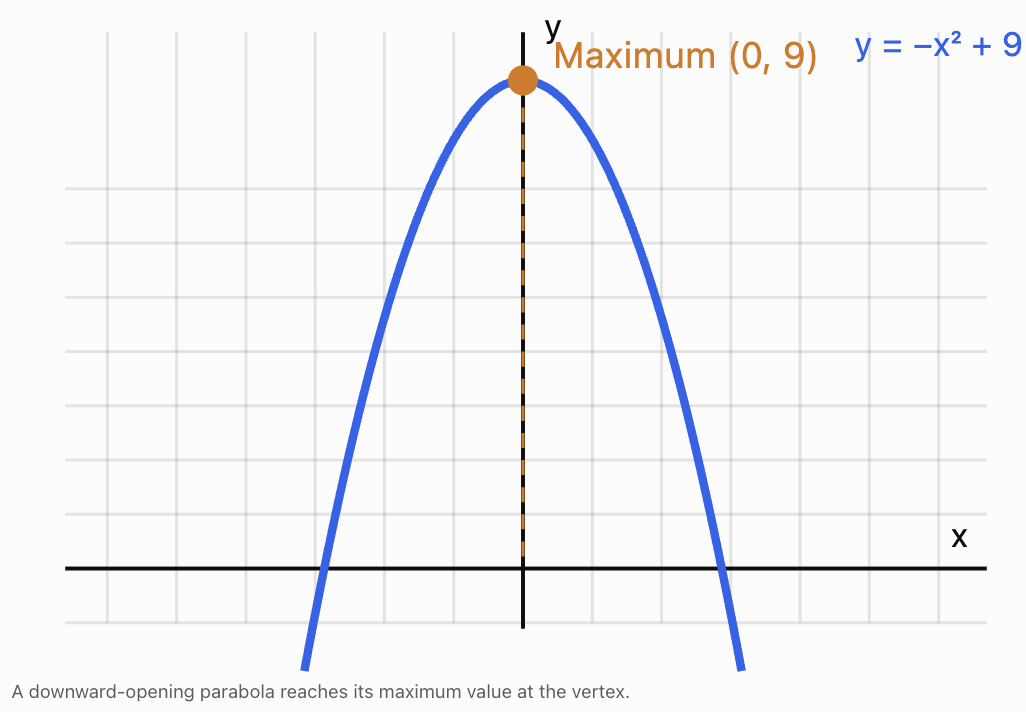
Consider the quadratic function:
f(x) = −x² + 9
Its graph is a downward-opening parabola.
The highest point is:
(0, 9)
Therefore:
-
The maximum value is 9.
-
The maximum occurs at x = 0.
-
The maximum point is (0, 9).
Notice the distinction between the maximum value and the point where it occurs.
The maximum value is a y-value.
The maximum point includes both the x-coordinate and the y-coordinate.
Maximum values and increasing or decreasing functions
For this graph:
-
The function increases as x approaches 0 from the left.
-
The function reaches its maximum at x = 0.
-
The function decreases as x moves to the right of 0.
A maximum often occurs where a graph changes from increasing to decreasing.
What Is a Minimum Value?
A minimum value is the smallest output a function reaches over a specified domain or interval.
Consider:
f(x) = x² − 4
The graph is an upward-opening parabola.
Its lowest point is:
(0, −4)
Therefore:
-
The minimum value is −4.
-
The minimum occurs at x = 0.
-
The minimum point is (0, −4).
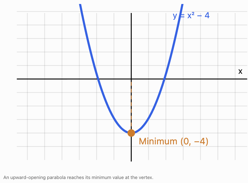
For this graph:
-
The function decreases until x = 0.
-
The function reaches its minimum.
-
The function then increases.
A minimum often occurs where a graph changes from decreasing to increasing.
Maximum and Minimum Points Versus Values
It is important to distinguish between three related ideas.
Consider:
f(x) = −2(x − 3)² + 10
The graph reaches its highest point at:
(3, 10)
We can describe this in three ways:
-
Maximum value: 10.
-
x-value where the maximum occurs: 3.
-
Maximum point: (3, 10).
These are not interchangeable.
If a question asks for the maximum value, the answer is 10.
If it asks where the maximum occurs, the answer is x = 3.
If it asks for the coordinates of the maximum point, the answer is (3, 10).
Local and Absolute Extrema
Not every maximum or minimum is the greatest or smallest value over an entire function.
We distinguish between local extrema and absolute extrema.
Local maximum
A local maximum occurs when a function's value is greater than or equal to nearby values.
The graph may rise to a peak, then fall.
However, another part of the graph may reach an even greater value.
Local minimum
A local minimum occurs when a function's value is less than or equal to nearby values.
The graph may fall into a valley, then rise.
However, another part of the graph may reach an even smaller value.
Absolute maximum
An absolute maximum is the greatest output of a function over its entire specified domain.
Absolute minimum
An absolute minimum is the smallest output of a function over its entire specified domain.
Type
Meaning
Local maximum
Greater than or equal to nearby outputs
Local minimum
Less than or equal to nearby outputs
Absolute maximum
Greatest output over the specified domain
Absolute minimum
Smallest output over the specified domain
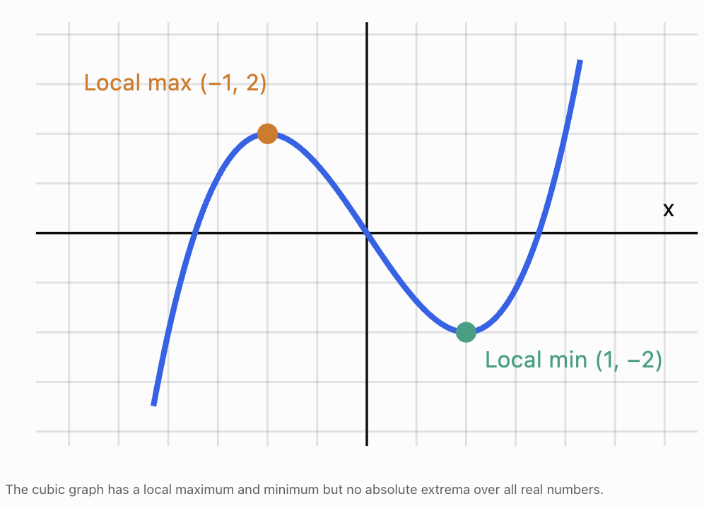
Example: A cubic function
Consider:
f(x) = x³ − 3x
This function has:
-
A local maximum at (−1, 2).
-
A local minimum at (1, −2).
However, over all real numbers, the function has no absolute maximum or absolute minimum.
As x becomes increasingly large and positive, f(x) increases without bound.
As x becomes increasingly negative, f(x) decreases without bound.
Turning Points
A turning point is a point where a graph changes direction.
There are two common types:
-
Increasing to decreasing: a local maximum.
-
Decreasing to increasing: a local minimum.
Identifying turning points visually
When reading a graph from left to right:
-
Find where the graph stops rising and starts falling.
-
Mark this as a possible local maximum.
-
Find where the graph stops falling and starts rising.
-
Mark this as a possible local minimum.
-
Read the coordinates of each point.
Turning points are especially important when analysing quadratic, cubic, and higher-degree polynomial functions.
Important distinction: Stationary points
A stationary point is a point where the derivative is zero, meaning the tangent is horizontal.
Some stationary points are turning points, but not all.
For example:
f(x) = x³
At x = 0, the graph has a horizontal tangent.
However, it continues increasing on both sides.
Therefore, (0, 0) is a stationary point but not a turning point.
Also, some turning points have sharp corners, such as the vertex of y = |x|, where the derivative is undefined.
This distinction becomes particularly important in calculus.
Finding Maximums and Minimums of Quadratic Functions
Quadratic functions are especially useful for studying extrema because their graphs have exactly one turning point.
The general form is:
f(x) = ax² + bx + c
where a ≠ 0.
The sign of a determines whether the vertex is a maximum or minimum.
-
If a > 0, the parabola opens upward and has a minimum.
-
If a < 0, the parabola opens downward and has a maximum.
The x-coordinate of the vertex is:
x = −b/(2a)
Once this x-value is known, substitute it into the function to find the maximum or minimum value.
Worked Example: Finding a minimum
Consider:
f(x) = 2x² − 12x + 11
Step 1: Identify the coefficients
a = 2
b = −12
c = 11
Because a is positive, the parabola opens upward.
Therefore, it has a minimum.
Step 2: Calculate the x-coordinate of the vertex
x = −b/(2a)
x = −(−12)/(2 × 2)
x = 12/4
x = 3
Step 3: Calculate the minimum value
Substitute x = 3:
f(3) = 2(3)² − 12(3) + 11
f(3) = 18 − 36 + 11
f(3) = −7
Answer:
-
Minimum value: −7
-
Minimum occurs at x = 3
-
Minimum point: (3, −7)
-
Axis of symmetry: x = 3
The function decreases on (−∞, 3) and increases on (3, ∞).
Worked Example: Finding a maximum
Consider:
g(x) = −3x² + 18x − 14
Because a = −3, the parabola opens downward.
The vertex occurs at:
x = −18/[2(−3)]
x = 3
Substitute:
g(3) = −3(3)² + 18(3) − 14
g(3) = −27 + 54 − 14
g(3) = 13
Answer:
-
Maximum value: 13
-
Maximum occurs at x = 3
-
Maximum point: (3, 13)
The function increases on (−∞, 3) and decreases on (3, ∞).
Finding Extrema Using Vertex Form
Quadratic functions can also be written in vertex form:
f(x) = a(x − h)² + k
The vertex is:
(h, k)
This makes it easy to identify the extremum without calculating −b/(2a).
Worked Example: Maximum
Consider:
f(x) = −4(x − 5)² + 20
The vertex is:
(5, 20)
Since a = −4, the parabola opens downward.
Therefore:
Maximum value = 20 at x = 5
Worked Example: Minimum
Consider:
g(x) = 0.5(x + 2)² − 6
Rewrite mentally as:
g(x) = 0.5(x − (−2))² − 6
The vertex is:
(−2, −6)
Since a = 0.5 is positive, the parabola opens upward.
Therefore:
Minimum value = −6 at x = −2
Why vertex form is useful
Vertex form makes three important properties immediately visible:
-
The horizontal position of the turning point.
-
The maximum or minimum value.
-
Whether the parabola opens upward or downward.
It is particularly useful in real-world optimisation problems.
Finding Extrema by Completing the Square
Sometimes a quadratic is given in standard form, but we want to rewrite it in vertex form.
This can be done by completing the square.
Worked Example
Find the minimum of:
f(x) = x² + 8x + 11
Start with:
f(x) = x² + 8x + 11
Half of 8 is 4.
Square 4 to get 16.
Rewrite:
f(x) = (x² + 8x + 16) − 16 + 11
Simplify:
f(x) = (x + 4)² − 5
The vertex is:
(−4, −5)
Because the squared expression cannot be negative:
(x + 4)² ≥ 0
Therefore:
(x + 4)² − 5 ≥ −5
The smallest possible output is −5.
Minimum value = −5 at x = −4
Completing the square does more than locate the vertex. It also explains algebraically why the value is a minimum.
Maximums and Minimums on Restricted Domains
A function's maximum and minimum values depend on the domain being considered.
For example:
f(x) = x²
Over all real numbers, the function has:
-
Absolute minimum: 0 at x = 0.
-
No absolute maximum.
However, suppose the domain is restricted to:
−2 ≤ x ≤ 3
Now the function has both an absolute minimum and an absolute maximum.
Calculate the important values:
f(−2) = 4
f(0) = 0
f(3) = 9
Therefore:
-
Absolute minimum: 0 at x = 0.
-
Absolute maximum: 9 at x = 3.
The maximum occurs at an endpoint, not at a turning point.
Worked Example: A restricted quadratic
Find the absolute maximum and minimum of:
f(x) = −x² + 4x + 1
on:
0 ≤ x ≤ 5
Step 1: Find the vertex
a = −1, b = 4
x = −4/[2(−1)]
x = 2
Step 2: Evaluate the vertex
f(2) = −4 + 8 + 1 = 5
Step 3: Evaluate the endpoints
f(0) = 1
f(5) = −25 + 20 + 1 = −4
Step 4: Compare
x
f(x)
0
1
2
5
5
−4
Therefore:
Absolute maximum = 5 at x = 2
Absolute minimum = −4 at x = 5
This example shows why checking only the vertex can give an incomplete answer.
For a continuous quadratic on a closed interval, evaluating the vertex when it lies inside the interval and evaluating both endpoints is sufficient to find its absolute extrema.
When a Maximum or Minimum Does Not Exist
Not every function reaches a greatest or smallest value.
Example: A linear function
Consider:
f(x) = 3x + 2
over all real numbers.
As x increases, f(x) increases without bound.
As x decreases, f(x) decreases without bound.
Therefore, the function has neither an absolute maximum nor an absolute minimum.
Example: An exponential function
Consider:
f(x) = 2ˣ
The function is always positive.
As x approaches negative infinity, its outputs approach zero.
However, the function never actually reaches zero.
Therefore:
-
It has no absolute minimum.
-
It has no absolute maximum.
Zero is the lower bound of its range, but it is not a minimum value.
Example: An open interval
Consider:
f(x) = x
with domain:
0 < x < 5
The function approaches zero and five but never reaches either endpoint.
Therefore, it has no absolute maximum or minimum on this domain.
This demonstrates an important distinction between a value that a function approaches and one that it actually reaches.
Finding Maximums and Minimums from Graphs
Sometimes we are given a graph without an equation.
In this situation, we estimate extrema visually.
Steps
-
Identify the domain shown on the graph.
-
Look for peaks and valleys.
-
Identify the x-coordinate of each peak or valley.
-
Read the corresponding y-value.
-
Determine whether each point is a local or absolute extremum.
-
Check the endpoints of the graph.
-
Use approximate values when the coordinates are not exact.
Example: A graph with several turning points
Suppose a graph has the following important points:
-
A local maximum at (−3, 5).
-
A local minimum at (0, −2).
-
Another local maximum at (4, 7).
The graph has at least two local maxima and one local minimum.
The greatest of the listed local maximum values is 7.
However, without knowing the entire graph and its domain, we cannot conclude that 7 is the absolute maximum.
Other parts of the function may reach greater values.
Estimating extrema from a graph
When a turning point lies between grid lines, estimate its coordinates.
For example, a maximum might appear near:
(2.4, 8.7)
We would write:
Approximate maximum value ≈ 8.7 at x ≈ 2.4
The approximation sign indicates that the coordinates were estimated rather than calculated exactly.
Comparing Extrema Across Different Functions
Maximum and minimum values provide useful information when comparing functions.
Consider three quadratic functions:
A: f(x) = −(x − 2)² + 8
B: g(x) = −2(x − 2)² + 12
C: h(x) = (x − 2)² − 3
Comparing their features
Feature
Function A
Function B
Function C
Opens
Downward
Downward
Upward
Vertex
(2, 8)
(2, 12)
(2, −3)
Extremum
Maximum
Maximum
Minimum
Extremum value
8
12
−3
x-value of extremum
2
2
2
Interpretation
Functions A and B both have maximum values, but B reaches a greater maximum.
Function C has a minimum rather than a maximum.
All three functions have their turning points at x = 2.
Therefore, their extrema occur at the same input value, even though their outputs and shapes differ.
Comparing graph widths
Function B has a larger absolute quadratic coefficient than Function A.
This means B is narrower.
However, the width of the parabola does not by itself determine the maximum or minimum value.
The vertical position of the vertex determines that value.
How Transformations Affect Extrema
Graph transformations are closely connected to maximums and minimums.
Start with:
f(x) = x²
Its minimum point is:
(0, 0)
Vertical translation
g(x) = x² + 5
The graph moves upward by 5.
The minimum changes from 0 to 5.
New minimum point:
(0, 5)
Horizontal translation
h(x) = (x − 3)²
The graph moves right by 3.
The minimum value remains 0, but it occurs at x = 3.
New minimum point:
(3, 0)
Reflection across the x-axis
p(x) = −x²
The graph is reflected vertically.
The original minimum becomes a maximum.
Maximum point:
(0, 0)
Vertical stretch
q(x) = 4(x − 2)² + 3
The graph is vertically stretched relative to the basic parabola, translated right by 2 and upward by 3.
Minimum point:
(2, 3)
The stretch changes the graph's width but does not change the vertex when applied to the squared term alone.
General conclusion
For:
y = a(x − h)² + k
-
h determines the horizontal position of the extremum.
-
k determines the extremum value.
-
The sign of a determines whether it is a maximum or minimum.
-
The magnitude of a determines the graph's vertical scaling.
Real-World Application: Maximum Height of a Projectile
Projectile motion is a common application of maximum values.
Suppose a ball is thrown upward from a platform.
Its height is modeled by:
h(t) = −5t² + 30t + 10
where:
-
h is height in metres.
-
t is time in seconds.
Step 1: Find the time of maximum height
The vertex occurs at:
t = −b/(2a)
a = −5, b = 30
t = −30/[2(−5)]
t = 3
Step 2: Find the maximum height
Substitute t = 3:
h(3) = −5(3)² + 30(3) + 10
h(3) = −45 + 90 + 10
h(3) = 55
Step 3: Interpret the result
Maximum height = 55 m
Time to maximum height = 3 s
The ball rises for the first 3 seconds, reaches its highest point, and then begins to fall.
This model assumes approximately constant gravitational acceleration and ignores air resistance.
Real-World Application: Maximum Business Profit
Businesses often try to identify the production or sales level that maximises profit.
Suppose profit is modeled by:
P(x) = −2x² + 120x − 1000
where:
-
x = number of products sold.
-
P(x) = profit in dollars.
Step 1: Determine the type of extremum
The coefficient of x² is negative.
Therefore, the parabola opens downward and has a maximum.
Step 2: Find the optimal sales quantity
x = −b/(2a)
x = −120/[2(−2)]
x = 30
Step 3: Find maximum profit
P(30) = −2(30)² + 120(30) − 1000
P(30) = −1800 + 3600 − 1000
P(30) = 800
Interpretation
Maximum modeled profit = $800
This occurs when 30 products are sold.
Selling fewer or more than 30 products produces a lower profit under the model.
The model is an idealised example; actual business decisions also depend on demand, production limits, and other costs.
Real-World Application: Minimising Costs
Not all optimisation problems involve finding a maximum.
Businesses and engineers often want to minimise costs.
Suppose the operating cost of a process is:
C(x) = 3(x − 12)² + 450
where x represents the number of operating hours per day.
The vertex is:
(12, 450)
Since the quadratic coefficient is positive, the graph opens upward.
Therefore:
Minimum cost = $450
This occurs at:
x = 12 hours
The model suggests that operating for either fewer or more than 12 hours increases the cost.
This might represent a process where very short operating periods create inefficiencies while very long periods lead to overtime or maintenance costs.
Real-World Application: Maximum Area
Optimisation is also important in geometry.
Suppose a farmer has 40 metres of fencing to enclose a rectangular field.
What dimensions give the greatest possible area?
Step 1: Write the perimeter equation
For a rectangle:
P = 2L + 2W
Since the perimeter is 40:
2L + 2W = 40
Divide by 2:
L + W = 20
Therefore:
L = 20 − W
Step 2: Write the area equation
Area = length × width
A = LW
Substitute L = 20 − W:
A(W) = W(20 − W)
Expand:
A(W) = −W² + 20W
Step 3: Find the maximum
The quadratic coefficient is negative, so the parabola opens downward.
The vertex occurs at:
W = −20/[2(−1)]
W = 10
Then:
L = 20 − 10
L = 10
Step 4: Calculate the area
A = 10 × 10
Maximum area = 100 m²
The greatest area occurs when the rectangle is a square measuring 10 m by 10 m.
Why this matters
The same mathematical idea can be applied to:
-
Designing gardens.
-
Minimising packaging materials.
-
Maximising storage capacity.
-
Optimising the dimensions of containers.
-
Reducing construction costs.
Real-World Application: Temperature Extremes
Suppose the temperature during part of a day is modeled by:
T(t) = −0.5(t − 14)² + 32
where t is the hour of the day.
The vertex is:
(14, 32)
The parabola opens downward.
Therefore:
Maximum temperature = 32°C at 14:00 (2:00 p.m.)
If the model applies only from 8:00 to 20:00, we can also determine the minimum over this interval.
At t = 8:
T(8) = −0.5(8 − 14)² + 32
T(8) = −18 + 32 = 14°C
At t = 20:
T(20) = −0.5(20 − 14)² + 32
T(20) = 14°C
Therefore, over the specified interval:
-
Maximum: 32°C at 14:00.
-
Minimum: 14°C at 8:00 and 20:00.
This is an illustrative temperature model rather than a prediction of actual weather.
Finding Extrema from Tables of Values
Sometimes a function is represented by a table rather than an equation or graph.
Consider the following measurements:
Time (min)
Temperature (°C)
0
18
5
23
10
28
15
31
20
29
25
24
30
20
The highest recorded temperature is 31°C at 15 minutes.
The lowest recorded temperature is 18°C at 0 minutes.
Therefore:
-
Recorded maximum: 31°C at 15 min.
-
Recorded minimum: 18°C at 0 min.
However, these are the extrema among the recorded measurements.
The temperature might have reached a slightly higher or lower value between measurements.
A continuous graph or mathematical model would be needed to investigate that possibility.
Comparing two datasets
Suppose two experiments produce the following results:
Time (min)
Experiment A
Experiment B
0
10
15
5
18
22
10
25
28
15
30
26
20
27
20
Experiment A has a recorded maximum of 30 at 15 minutes.
Experiment B has a recorded maximum of 28 at 10 minutes.
Therefore:
-
Experiment A reaches a higher recorded maximum.
-
Experiment B reaches its recorded maximum earlier.
-
The experiments have different trends after reaching their peaks.
Comparing extrema helps us understand not only how high or low a quantity becomes but also when important events occur.
Extrema of Other Function Families
Quadratic functions are not the only functions that can have maximums or minimums.
Absolute value functions
Consider:
f(x) = |x − 3| + 2
The graph has a V shape.
Its vertex is:
(3, 2)
Therefore:
Minimum value = 2 at x = 3
Now consider:
g(x) = −|x + 1| + 5
This graph is an upside-down V.
Its vertex is:
(−1, 5)
Therefore:
Maximum value = 5 at x = −1
These are examples of extrema at sharp turning points.
Cubic functions
Consider:
f(x) = x³ − 3x
The function has a local maximum at (−1, 2) and a local minimum at (1, −2).
Unlike a quadratic, it has more than one turning point.
Trigonometric functions
Consider:
f(x) = sin x
The sine function repeatedly reaches:
-
Maximum value: 1.
-
Minimum value: −1.
These extrema repeat periodically.
For a transformed sine function:
g(x) = 3 sin x + 2
The amplitude is 3 and the midline is y = 2.
Therefore:
Maximum = 2 + 3 = 5
Minimum = 2 − 3 = −1
Exponential functions
Consider:
f(x) = 2ˣ
Over all real numbers, this function has no maximum or minimum.
It increases without bound and approaches zero without reaching it.
These examples demonstrate that extrema depend on the function's shape and domain.
An Introduction to Calculus and Extrema
For more advanced functions, calculus provides a systematic method for locating possible extrema.
The derivative measures the instantaneous rate of change of a function.
It is commonly written as:
f′(x)
For a smooth function:
-
f′(x) > 0 means the function is increasing locally.
-
f′(x) < 0 means the function is decreasing locally.
-
f′(x) = 0 identifies a stationary point.
A stationary point may be a local maximum, local minimum, or neither.
Worked Example: Using the derivative
Consider:
f(x) = x³ − 3x
Differentiate:
f′(x) = 3x² − 3
Set the derivative equal to zero:
3x² − 3 = 0
3x² = 3
x² = 1
x = −1 or x = 1
These are the stationary points.
Evaluate the function:
f(−1) = (−1)³ − 3(−1)
f(−1) = −1 + 3 = 2
f(1) = 1 − 3 = −2
The stationary points are:
(−1, 2) and (1, −2)
Now examine the sign of the derivative:
Interval
Sign of f′(x)
Behaviour
x < −1
Positive
Increasing
−1 < x < 1
Negative
Decreasing
x > 1
Positive
Increasing
Therefore:
-
At x = −1, the function changes from increasing to decreasing: local maximum.
-
At x = 1, the function changes from decreasing to increasing: local minimum.
Important limitation
Finding f′(x) = 0 identifies possible extrema, but it does not guarantee an extremum.
We must also check where the derivative changes sign or use another appropriate test.
For absolute extrema on a closed interval, endpoints must also be considered.
For functions with corners or other nondifferentiable points, extrema can occur even when the derivative does not exist.
A Step-by-Step Strategy for Finding Extrema
When solving a maximum or minimum problem, use the following approach.
Identify the function.
Determine the equation or graph representing the quantity.
Identify the domain.
Decide which input values are allowed or meaningful.
Locate possible extrema.
For quadratics, find the vertex.
For graphs, identify peaks, valleys, and relevant endpoints.
For more advanced functions, investigate stationary points and points where the derivative is undefined.
Calculate the output values.
Substitute the relevant x-values into the function.
Compare the values.
Determine which is greatest or smallest over the specified domain.
Interpret the result.
Explain the meaning using appropriate units.
Check whether the result is realistic.
Consider restrictions such as time, cost, distance, and production capacity.
Common Mistakes
Confusing the maximum value with the x-coordinate where it occurs
If the maximum point is (3, 10), the maximum value is 10, not 3.
Assuming every turning point is an absolute extremum
A turning point may be only a local maximum or minimum.
Ignoring the domain
A function may have different extrema when its domain is restricted.
Forgetting to check endpoints
Absolute extrema on a closed interval may occur at endpoints.
Assuming every function has a maximum and minimum
Some functions increase or decrease without bound.
Confusing the sign of the vertex's y-coordinate with the type of extremum
A negative value can be a maximum, and a positive value can be a minimum.
Assuming all stationary points are turning points
The function y = x³ has a stationary point at the origin but no turning point there.
Misidentifying the direction of a parabola
For y = ax² + bx + c, a positive coefficient gives a minimum, while a negative coefficient gives a maximum.
Ignoring units in real-world problems
A maximum height must be expressed in units of length, while maximum profit is expressed in currency.
Treating recorded data extrema as exact continuous extrema
The greatest measured value may not be the greatest value reached between measurements.
Key Terms
-
Maximum value: The greatest output of a function over a specified domain.
-
Minimum value: The smallest output of a function over a specified domain.
-
Extremum: A maximum or minimum.
-
Extrema: The plural of extremum.
-
Local maximum: A value greater than or equal to nearby function values.
-
Local minimum: A value less than or equal to nearby function values.
-
Absolute maximum: The greatest output over the entire specified domain.
-
Absolute minimum: The smallest output over the entire specified domain.
-
Turning point: A point where a graph changes from increasing to decreasing or vice versa.
-
Vertex: The turning point of a parabola.
-
Axis of symmetry: A line dividing a symmetric graph into matching halves.
-
Stationary point: A point where the derivative equals zero.
-
Derivative: A measure of the instantaneous rate of change of a function.
-
Critical point: An interior point where the derivative is zero or undefined, under the usual calculus definition.
-
Optimisation: The process of finding the greatest or smallest possible value of a quantity.
-
Restricted domain: A specified subset of permitted input values.
-
Endpoint: A boundary value of an interval.
-
Quadratic function: A function with a squared variable as its highest power.
-
Vertex form: A quadratic equation written as y = a(x − h)² + k.
-
Completing the square: An algebraic method for rewriting a quadratic expression in squared form.
Key Takeaways
-
Maximums and minimums describe the greatest and smallest outputs of functions.
-
A maximum or minimum value is a y-value, while an extremum point includes both coordinates.
-
Local extrema describe behaviour near a point.
-
Absolute extrema describe the greatest or smallest values over the specified domain.
-
Turning points often occur where a graph changes between increasing and decreasing.
-
Upward-opening parabolas have a minimum at the vertex.
-
Downward-opening parabolas have a maximum at the vertex.
-
The vertex of y = ax² + bx + c occurs at x = −b/(2a).
-
Vertex form y = a(x − h)² + k makes the extremum easy to identify.
-
Restricted domains can change the absolute maximum and minimum.
-
Endpoints must be considered when finding absolute extrema on closed intervals.
-
Some functions have no absolute maximum or minimum.
-
Extrema are useful for solving real-world optimisation problems.
-
Comparing extrema helps us evaluate different functions, models, and situations.
Check Your Understanding
Recall and Understanding
1. Explain the difference between a maximum value and a maximum point.
2. What is the difference between a local maximum and an absolute maximum?
3. Describe how to identify a minimum point from a graph.
4. Explain why a linear function such as y = 3x + 2 has no absolute maximum or minimum over all real numbers.
Application
5. Find the minimum value and vertex of f(x) = x² − 8x + 10.
6. Find the maximum value and vertex of g(x) = −2x² + 12x − 7.
7. Identify the extremum of h(x) = 3(x − 4)² + 6.
8. Identify the extremum of p(x) = −5(x + 2)² + 11.
9. Find the absolute maximum and minimum of f(x) = x² − 4x + 1 on the interval 0 ≤ x ≤ 5.
10. Determine the maximum and minimum values of y = 4 sin x − 3.
Analysis and Challenge
11. A ball's height is modeled by h(t) = −5t² + 40t + 3. Find its maximum height and the time at which it occurs.
12. A company's profit is modeled by P(x) = −4x² + 160x − 900. Find the production quantity that maximises profit and calculate the maximum profit.
13. A rectangle has a perimeter of 60 cm. Find the dimensions that maximise its area and calculate that area.
14. Compare the extrema of:
A: f(x) = −(x − 3)² + 12
B: g(x) = −3(x − 3)² + 18
C: h(x) = 2(x − 3)² − 5
15. A student claims that the function f(x) = x³ − 3x has an absolute maximum at (−1, 2) because this point is a local maximum. Explain why the claim is incorrect.
Answers to Check Your Understanding
1. The maximum value is the greatest y-value of a function over a specified domain. The maximum point gives both the x-coordinate where it occurs and the maximum y-value.
For example, if the maximum point is (4, 10), the maximum value is 10.
2. A local maximum is greater than or equal to nearby outputs. An absolute maximum is the greatest output over the entire specified domain.
3. Look for a point where the graph stops decreasing and begins increasing. This is a local minimum. To determine whether it is an absolute minimum, compare it with all other relevant values, including endpoints.
4. The function y = 3x + 2 increases without bound as x increases and decreases without bound as x decreases. Therefore, it has neither an absolute maximum nor an absolute minimum over all real numbers.
5.
f(x) = x² − 8x + 10
a = 1, b = −8
x = −b/(2a)
x = 8/2 = 4
Substitute:
f(4) = 16 − 32 + 10
f(4) = −6
Minimum value = −6
Vertex = (4, −6)
6.
g(x) = −2x² + 12x − 7
a = −2, b = 12
x = −12/[2(−2)]
x = 3
Substitute:
g(3) = −2(9) + 12(3) − 7
g(3) = −18 + 36 − 7
g(3) = 11
Maximum value = 11
Vertex = (3, 11)
7.
h(x) = 3(x − 4)² + 6
The vertex is (4, 6).
Because the quadratic coefficient is positive, the parabola opens upward.
Minimum value = 6 at x = 4
8.
p(x) = −5(x + 2)² + 11
The vertex is (−2, 11).
Because the quadratic coefficient is negative, the parabola opens downward.
Maximum value = 11 at x = −2
9.
f(x) = x² − 4x + 1
Domain:
0 ≤ x ≤ 5
Find the vertex:
x = −(−4)/(2 × 1) = 2
Evaluate:
f(0) = 1
f(2) = 4 − 8 + 1 = −3
f(5) = 25 − 20 + 1 = 6
Compare:
-
f(0) = 1
-
f(2) = −3
-
f(5) = 6
Absolute minimum = −3 at x = 2
Absolute maximum = 6 at x = 5
10.
y = 4 sin x − 3
Since:
−1 ≤ sin x ≤ 1
Multiplying by 4:
−4 ≤ 4 sin x ≤ 4
Subtracting 3:
−7 ≤ 4 sin x − 3 ≤ 1
Therefore:
Maximum value = 1
Minimum value = −7
11.
h(t) = −5t² + 40t + 3
Find the vertex:
t = −40/[2(−5)]
t = 4
Calculate:
h(4) = −5(4)² + 40(4) + 3
h(4) = −80 + 160 + 3
h(4) = 83
Maximum height = 83 m
Time to maximum height = 4 s
12.
P(x) = −4x² + 160x − 900
The vertex occurs at:
x = −160/[2(−4)]
x = 20
Substitute:
P(20) = −4(20)² + 160(20) − 900
P(20) = −1600 + 3200 − 900
P(20) = 700
Optimal production quantity = 20 products
Maximum modeled profit = $700
13.
Let the rectangle have length L and width W.
Perimeter:
2L + 2W = 60
L + W = 30
L = 30 − W
Area:
A = LW
A(W) = W(30 − W)
A(W) = −W² + 30W
Find the vertex:
W = −30/[2(−1)]
W = 15
Therefore:
L = 30 − 15 = 15
Area:
A = 15 × 15 = 225
Dimensions = 15 cm × 15 cm
Maximum area = 225 cm²
14.
Function
Vertex
Extremum
A
(3, 12)
Maximum of 12
B
(3, 18)
Maximum of 18
C
(3, −5)
Minimum of −5
All three functions have their extrema at x = 3.
Function B has the greatest maximum value.
Function C opens upward and therefore has a minimum rather than a maximum.
Function B is narrower than Function A because its quadratic coefficient has a greater absolute value.
15.
The function:
f(x) = x³ − 3x
has a local maximum at (−1, 2).
However, it continues increasing without bound as x approaches positive infinity.
Therefore, there are values of x for which f(x) is greater than 2.
The point (−1, 2) is only a local maximum.
The function has no absolute maximum over all real numbers.
Final Summary
Maximums and minimums are essential features of functions because they help identify the greatest and smallest possible values of quantities.
By locating turning points, analysing quadratic equations, examining graphs, and considering restricted domains, we can determine where extrema occur and what they mean.
These skills are particularly important in optimisation problems involving height, profit, cost, area, temperature, and other real-world quantities.
The central idea is that finding an extremum requires understanding both the value of a function and the domain over which that value is being compared.
-
4. Function Features
Learning outcomes
- I can identify symmetry.
- I can identify intervals of positive and negative values.
- I can describe end behavior.
- I can compare important graph features.
- I can summarize the behavior of a graph.
Introduction
A graph provides much more information than simply showing how two variables are related. By examining its shape, position, intercepts, turning points, and overall direction, we can understand the behaviour of a function without calculating every possible output.
For example, consider the quadratic function:
f(x) = x² − 4
From its graph, we can determine that:
-
It is symmetric about the y-axis.
-
It has x-intercepts at (−2, 0) and (2, 0).
-
It has a minimum value of −4 at x = 0.
-
It is positive when x < −2 or x > 2.
-
It is negative when −2 < x < 2.
-
Both ends of the graph rise toward positive infinity.
These characteristics are called function features.
Understanding function features allows us to describe, compare, and interpret mathematical relationships in a systematic way.
This is useful in many areas of mathematics, including algebra, calculus, statistics, and mathematical modelling.
It is also important in science, engineering, economics, and other subjects where graphs are used to represent changing quantities.
What Are Function Features?
Function features are the important mathematical characteristics that describe a function's graph and behaviour.
Common features include:
-
Domain and range.
-
x-intercepts and y-intercepts.
-
Symmetry.
-
Increasing and decreasing intervals.
-
Maximum and minimum values.
-
Positive and negative intervals.
-
End behaviour.
-
Turning points.
-
Asymptotes.
-
Continuity.
Different function families have different combinations of these features.
For example, a straight line may have no turning points, while a quadratic function has one turning point.
A cubic function may have two turning points, and an exponential function may approach an asymptote without crossing it.
By identifying these features, we can build a complete mathematical description of a graph.
Symmetry of Functions
A graph has symmetry when parts of it match under a reflection or rotation.
Symmetry helps us understand graph shapes and predict values without calculating every point.
Two particularly important types of symmetry are:
-
Symmetry about the y-axis.
-
Symmetry about the origin.
These are associated with even functions and odd functions.
Even Functions: Symmetry About the y-Axis
An even function has a graph that is symmetric about the y-axis.
This means the left and right sides are mirror images.
The mathematical condition is:
f(−x) = f(x)
for every x in the domain.
The domain must also be symmetric about zero.
Example: A quadratic function
Consider:
f(x) = x²
Calculate:
f(2) = 2² = 4
f(−2) = (−2)² = 4
Therefore:
f(−2) = f(2)
The same relationship holds for every real x.
The function is even.
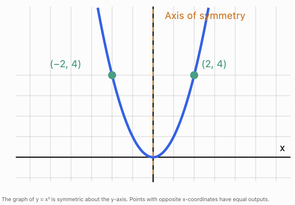
Other examples of even functions
-
f(x) = x⁴
-
f(x) = |x|
-
f(x) = cos x
-
f(x) = x² + 5
-
f(x) = 3x⁴ − 2x² + 1
For example:
f(x) = 3x⁴ − 2x² + 1
Substitute −x:
f(−x) = 3(−x)⁴ − 2(−x)² + 1
Because even powers remove negative signs:
f(−x) = 3x⁴ − 2x² + 1
Therefore:
f(−x) = f(x)
The function is even.
Odd Functions: Symmetry About the Origin
An odd function has symmetry about the origin.
This means that rotating its graph 180° around the origin produces the same graph.
The mathematical condition is:
f(−x) = −f(x)
for every x in the domain.
Example: A cubic function
Consider:
f(x) = x³
Calculate:
f(2) = 8
f(−2) = −8
Therefore:
f(−2) = −f(2)
The same relationship holds for every real x.
The function is odd.
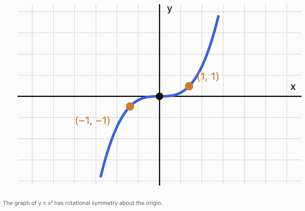
Other examples of odd functions
-
f(x) = x
-
f(x) = x⁵
-
f(x) = sin x
-
f(x) = 1/x, for x ≠ 0
-
f(x) = x³ − 4x
Worked Example
Determine whether:
f(x) = x³ − 4x
is odd.
Substitute −x:
f(−x) = (−x)³ − 4(−x)
f(−x) = −x³ + 4x
Factor out −1:
f(−x) = −(x³ − 4x)
Therefore:
f(−x) = −f(x)
The function is odd.
Functions That Are Neither Even Nor Odd
Some functions have neither y-axis symmetry nor origin symmetry.
Consider:
f(x) = x² + x
Substitute −x:
f(−x) = x² − x
This is not equal to f(x).
It is also not equal to −f(x).
Therefore, the function is neither even nor odd.
Important distinction
A graph can have a line of symmetry without being an even function.
For example:
f(x) = (x − 3)²
has a vertical line of symmetry:
x = 3
However, it is not symmetric about the y-axis, so it is not an even function.
Similarly, some graphs have rotational symmetry around a point other than the origin without being odd functions.
Symmetry comparison
|
Feature |
Even function |
Odd function |
|---|---|---|
|
Symmetry |
y-axis |
Origin |
|
Algebraic test |
f(−x) = f(x) |
f(−x) = −f(x) |
|
Typical example |
x² |
x³ |
|
Matching points |
(x, y) and (−x, y) |
(x, y) and (−x, −y) |
The zero function f(x) = 0 is a special case: it is both even and odd.
Positive and Negative Intervals
Another important feature of a function is whether its outputs are positive or negative.
A function is positive wherever its graph lies above the x-axis.
A function is negative wherever its graph lies below the x-axis.
Mathematically:
-
Positive: f(x) > 0
-
Negative: f(x) < 0
-
Zero: f(x) = 0
These intervals describe the sign of the function's outputs, not whether the graph is increasing or decreasing.
A function can be positive and decreasing at the same time.
Worked Example: A linear function
Consider:
f(x) = 2x − 6
First, find the x-intercept:
0 = 2x − 6
x = 3
The graph crosses the x-axis at (3, 0).
For x > 3:
2x − 6 > 0
Therefore, the function is positive.
For x < 3:
2x − 6 < 0
Therefore, the function is negative.
Positive interval: (3, ∞)
Negative interval: (−∞, 3)
At x = 3, the function equals zero, so this point belongs to neither interval.
Finding Positive and Negative Intervals of Quadratic Functions
Quadratic functions can have several sign patterns depending on their roots and the direction in which they open.
Worked Example: An upward-opening parabola
Consider:
f(x) = x² − 4
Factor:
f(x) = (x − 2)(x + 2)
The roots are:
x = −2 and x = 2
These divide the number line into three intervals:
-
x < −2
-
−2 < x < 2
-
x > 2
Test one value in each interval.
|
Interval |
Test x |
f(x) |
Sign |
|---|---|---|---|
|
x < −2 |
−3 |
5 |
Positive |
|
−2 < x < 2 |
0 |
−4 |
Negative |
|
x > 2 |
3 |
5 |
Positive |
Therefore:
Positive: (−∞, −2) and (2, ∞)
Negative: (−2, 2)
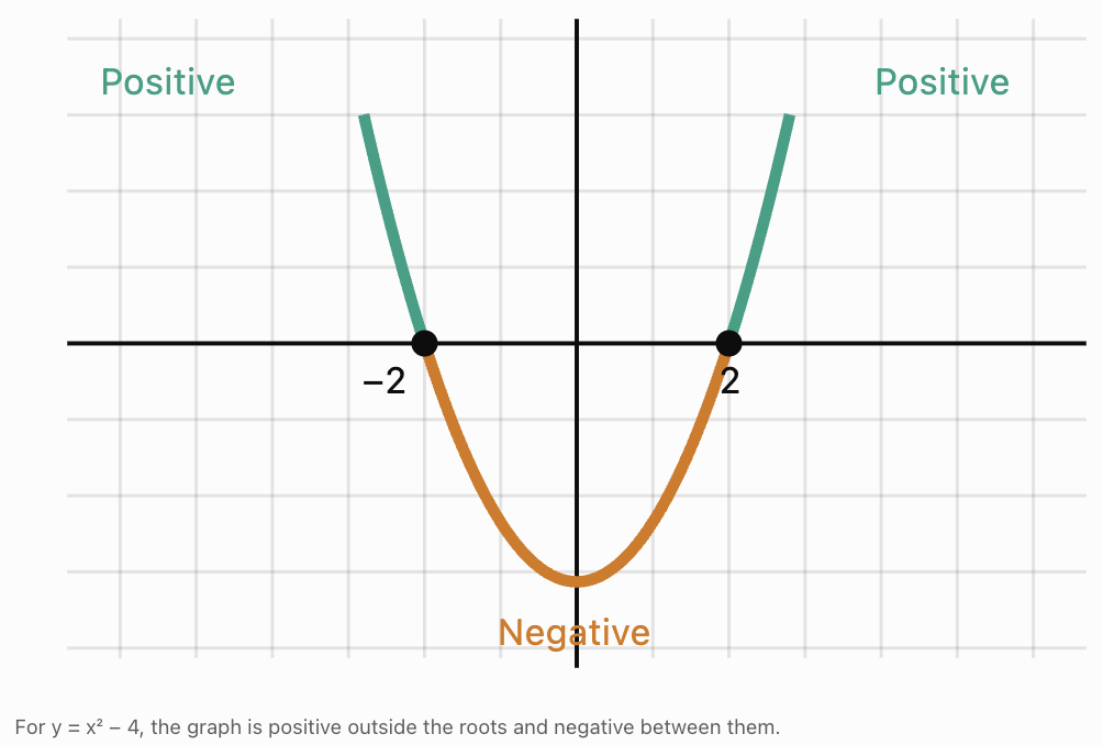
Worked Example: A downward-opening parabola
Consider:
g(x) = −x² + 9
Find the roots:
0 = −x² + 9
x² = 9
x = −3 or x = 3
Since the parabola opens downward, its graph lies above the x-axis between the roots and below the x-axis outside them.
Therefore:
Positive: (−3, 3)
Negative: (−∞, −3) and (3, ∞)
A parabola that never crosses the x-axis
Consider:
h(x) = x² + 2
Since x² ≥ 0:
x² + 2 ≥ 2
Therefore, the function is positive for every real x.
Positive: (−∞, ∞)
Negative: None
This demonstrates that a function does not need x-intercepts to have positive or negative intervals.
Sign Charts
A sign chart is a useful tool for identifying where a function is positive, negative, or zero.
Consider:
f(x) = (x + 3)(x − 1)
The roots are x = −3 and x = 1.
|
Interval |
x + 3 |
x − 1 |
f(x) |
|---|---|---|---|
|
x < −3 |
Negative |
Negative |
Positive |
|
−3 < x < 1 |
Positive |
Negative |
Negative |
|
x > 1 |
Positive |
Positive |
Positive |
Multiplying two negative numbers gives a positive result.
Multiplying a positive number and a negative number gives a negative result.
Therefore:
Positive: (−∞, −3) and (1, ∞)
Negative: (−3, 1)
Sign charts are particularly useful for polynomial and rational functions.
For rational functions, remember to exclude any values where the denominator equals zero.
Distinguishing Sign from Direction of Change
One of the most important skills in graph analysis is distinguishing between the sign of a function and whether it is increasing or decreasing.
Consider:
f(x) = −x + 5
This function is decreasing everywhere because its gradient is −1.
However:
-
It is positive for x < 5.
-
It equals zero at x = 5.
-
It is negative for x > 5.
The function is therefore positive and decreasing on (−∞, 5).
Similarly, the function:
g(x) = x − 5
is increasing everywhere but negative when x < 5.
|
Feature |
Question being answered |
|---|---|
|
Positive or negative |
Is the graph above or below the x-axis? |
|
Increasing or decreasing |
Does the graph rise or fall from left to right? |
|
Maximum or minimum |
Where does the graph reach a high or low value? |
These are different properties and should be analysed separately.
End Behaviour of Functions
End behaviour describes what happens to a function's outputs as x becomes very large and positive or very large and negative.
We examine two directions:
-
As x approaches positive infinity.
-
As x approaches negative infinity.
The symbol ∞ represents infinity.
The symbol −∞ represents negative infinity.
Infinity is not a number that a function eventually reaches. Instead, these expressions describe what happens as the input grows without bound.
End behaviour notation
We commonly write:
As x → ∞, f(x) → ∞
This means that as x becomes increasingly large and positive, the output increases without bound.
Similarly:
As x → −∞, f(x) → −∞
means that as x becomes increasingly large in the negative direction, the output decreases without bound.
End behaviour helps us understand the overall shape of a graph, especially outside the visible plotting window.
End Behaviour of Linear Functions
Consider:
f(x) = 2x + 3
The gradient is positive.
Therefore:
-
As x → ∞, f(x) → ∞.
-
As x → −∞, f(x) → −∞.
Now consider:
g(x) = −2x + 3
The gradient is negative.
Therefore:
-
As x → ∞, g(x) → −∞.
-
As x → −∞, g(x) → ∞.
The sign of the gradient determines the end behaviour of a nonconstant linear function.
End Behaviour of Quadratic Functions
For:
f(x) = ax² + bx + c
the sign of a determines the end behaviour.
Positive leading coefficient
If a > 0, the parabola opens upward.
Both ends rise:
As x → ∞, f(x) → ∞
As x → −∞, f(x) → ∞
Example:
f(x) = x² − 4x + 1
Negative leading coefficient
If a < 0, the parabola opens downward.
Both ends fall:
As x → ∞, f(x) → −∞
As x → −∞, f(x) → −∞
Example:
g(x) = −2x² + 3x + 5
The lower-degree terms affect the position and shape of the graph but do not change its end behaviour.
End Behaviour of Polynomial Functions
For polynomial functions, the highest-power term usually determines the end behaviour.
This term is called the leading term.
For example:
f(x) = 3x⁴ − 2x³ + 5x − 7
The leading term is:
3x⁴
Because the degree is even and the leading coefficient is positive, both ends rise.
Four common end behaviour patterns
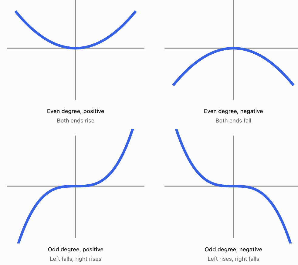
Summary table
|
Degree |
Leading coefficient |
Left end |
Right end |
|---|---|---|---|
|
Even |
Positive |
Rises |
Rises |
|
Even |
Negative |
Falls |
Falls |
|
Odd |
Positive |
Falls |
Rises |
|
Odd |
Negative |
Rises |
Falls |
Worked Example
Describe the end behaviour of:
f(x) = −4x⁵ + 3x² − 8
The leading term is:
−4x⁵
The degree is odd.
The leading coefficient is negative.
Therefore:
As x → −∞, f(x) → ∞
As x → ∞, f(x) → −∞
The graph rises on the left and falls on the right.
End Behaviour of Exponential Functions
Exponential functions behave differently from polynomials.
Consider:
f(x) = 2ˣ
As x becomes increasingly large:
f(x) increases without bound.
Therefore:
As x → ∞, f(x) → ∞
As x becomes increasingly negative:
f(x) approaches zero from above.
Therefore:
As x → −∞, f(x) → 0
The line y = 0 is a horizontal asymptote.
Exponential decay
Consider:
g(x) = (1/2)ˣ
As x → ∞:
g(x) → 0
As x → −∞:
g(x) → ∞
The function decreases from left to right and approaches zero on the right.
Vertical translations and asymptotes
Consider:
h(x) = 2ˣ + 3
This is the graph of 2ˣ translated upward by 3 units.
Its horizontal asymptote is:
y = 3
Therefore:
As x → −∞, h(x) → 3.
As x → ∞, h(x) → ∞.
The vertical translation changes the horizontal asymptote but does not change the overall direction of exponential growth.
End Behaviour of Rational Functions
Rational functions are ratios of polynomial expressions.
Consider:
f(x) = 1/x
As x becomes very large and positive:
f(x) approaches zero from above.
As x becomes very large and negative:
f(x) approaches zero from below.
Therefore:
-
As x → ∞, f(x) → 0.
-
As x → −∞, f(x) → 0.
The graph has a horizontal asymptote:
y = 0
It also has a vertical asymptote at:
x = 0
The function is undefined at x = 0.
Worked Example
Consider:
g(x) = 3 + 2/x
As x → ∞:
2/x → 0
Therefore:
g(x) → 3
As x → −∞:
2/x → 0
Therefore:
g(x) → 3
The horizontal asymptote is:
y = 3
This illustrates how a function can approach a finite value at both ends rather than increasing or decreasing without bound.
End Behaviour of Trigonometric Functions
Periodic functions such as sine and cosine behave differently again.
Consider:
f(x) = sin x
The function repeatedly oscillates between −1 and 1.
As x approaches positive or negative infinity, the function continues oscillating.
It does not approach one particular value.
Therefore, sin x has no single limiting value as x → ∞ or x → −∞.
This demonstrates that not all functions have end behaviour described by approaching infinity or a horizontal asymptote.
Comparing Important Graph Features
When comparing functions, it is useful to organise the information into a table.
Consider these four functions:
A: f(x) = x²
B: g(x) = −x²
C: h(x) = x³
D: p(x) = 2ˣ
Comparison table
|
Feature |
x² |
−x² |
x³ |
2ˣ |
|---|---|---|---|---|
|
Domain |
All real numbers |
All real numbers |
All real numbers |
All real numbers |
|
Range |
y ≥ 0 |
y ≤ 0 |
All real numbers |
y > 0 |
|
Symmetry |
Even |
Even |
Odd |
Neither |
|
x-intercept |
(0, 0) |
(0, 0) |
(0, 0) |
None |
|
y-intercept |
(0, 0) |
(0, 0) |
(0, 0) |
(0, 1) |
|
Extremum |
Minimum 0 |
Maximum 0 |
None |
None |
|
Positive intervals |
x ≠ 0 |
None |
x > 0 |
All real x |
|
Negative intervals |
None |
x ≠ 0 |
x < 0 |
None |
Comparing their end behaviour
f(x) = x²
Both ends rise.
g(x) = −x²
Both ends fall.
h(x) = x³
The left end falls and the right end rises.
p(x) = 2ˣ
The left end approaches zero, while the right end rises without bound.
Why comparisons matter
Although these functions may pass through some of the same points, their overall behaviour is very different.
For example, x² and x³ both pass through the origin, but:
-
x² is even.
-
x³ is odd.
-
x² has a minimum.
-
x³ has no local or absolute extrema over all real numbers.
-
x² is never negative.
-
x³ is negative for negative x-values.
Comparing several features gives a more complete understanding than looking at intercepts alone.
Summarising the Behaviour of a Graph
A complete graph description should combine several important features.
Rather than listing disconnected facts, we can explain how the function behaves as a whole.
Worked Example: A quadratic function
Consider:
f(x) = x² − 6x + 5
We will analyse its important features.
Finding the intercepts
For the x-intercepts, set f(x) = 0:
x² − 6x + 5 = 0
Factor:
(x − 1)(x − 5) = 0
Therefore:
x = 1 or x = 5
x-intercepts: (1, 0) and (5, 0)
For the y-intercept:
f(0) = 5
y-intercept: (0, 5)
Finding the turning point
Use:
x = −b/(2a)
Here a = 1 and b = −6.
x = 6/2 = 3
Substitute:
f(3) = 9 − 18 + 5
f(3) = −4
Vertex: (3, −4)
Since the parabola opens upward, this is a minimum.
Finding the symmetry
The axis of symmetry is:
x = 3
The graph is symmetric about this vertical line.
However, the function is neither even nor odd because it is not symmetric about the y-axis or origin.
Finding the positive and negative intervals
The roots are x = 1 and x = 5.
The parabola opens upward.
Therefore:
Positive: (−∞, 1) and (5, ∞)
Negative: (1, 5)
Finding increasing and decreasing intervals
The vertex occurs at x = 3.
Therefore:
Decreasing: (−∞, 3)
Increasing: (3, ∞)
Describing end behaviour
The leading term is x².
It has even degree and a positive leading coefficient.
Therefore:
-
As x → −∞, f(x) → ∞.
-
As x → ∞, f(x) → ∞.
Complete graph summary
|
Feature |
Description |
|---|---|
|
Function |
f(x) = x² − 6x + 5 |
|
Domain |
All real numbers |
|
Range |
y ≥ −4 |
|
x-intercepts |
(1, 0), (5, 0) |
|
y-intercept |
(0, 5) |
|
Minimum |
−4 at x = 3 |
|
Axis of symmetry |
x = 3 |
|
Even or odd |
Neither |
|
Increasing |
(3, ∞) |
|
Decreasing |
(−∞, 3) |
|
Positive |
(−∞, 1), (5, ∞) |
|
Negative |
(1, 5) |
|
End behaviour |
Both ends rise |
This is a complete mathematical description of the function's main features.
Real-World Application: Projectile Motion
A ball is thrown upward from a platform.
Its height is modeled by:
h(t) = −5t² + 20t + 5
where:
-
t is time in seconds.
-
h is height in metres.
Initial height
At t = 0:
h(0) = 5
The ball begins 5 m above the ground.
Maximum height
The vertex occurs at:
t = −20/[2(−5)]
t = 2
Calculate:
h(2) = −5(2)² + 20(2) + 5
h(2) = −20 + 40 + 5
h(2) = 25
Maximum height = 25 m at t = 2 s
When the ball reaches the ground
Set h(t) = 0:
−5t² + 20t + 5 = 0
Divide by −5:
t² − 4t − 1 = 0
Using the quadratic formula:
t = 2 ± √5
The positive solution is:
t ≈ 4.24 s
Interpreting the function features
Over the physical flight:
-
Height increases from t = 0 to t = 2 s.
-
Maximum height is 25 m.
-
Height decreases from t = 2 s to approximately t = 4.24 s.
-
Height is positive before the ball lands.
-
Height equals zero when the ball reaches the ground.
Although the mathematical quadratic has end behaviour extending to infinity, this is not physically meaningful for the ball's actual flight.
The practical domain is approximately:
0 ≤ t ≤ 4.24
This illustrates why real-world models must be interpreted within appropriate domains.
Real-World Application: Business Profit
Suppose a business models its profit using:
P(x) = −2(x − 30)² + 1800
where:
-
x is the number of products sold.
-
P(x) is profit in dollars.
Maximum profit
The vertex is:
(30, 1800)
Therefore:
Maximum modeled profit = $1,800
This occurs when 30 products are sold.
Positive and negative profit
A positive profit means the business earns more revenue than its costs.
A negative profit means the business operates at a loss.
Find the break-even points by setting P(x) = 0:
0 = −2(x − 30)² + 1800
2(x − 30)² = 1800
(x − 30)² = 900
x − 30 = ±30
x = 0 or x = 60
Therefore:
-
Profit is positive for 0 < x < 60.
-
Profit equals zero at x = 0 and x = 60.
-
The mathematical model gives negative profit for x > 60.
Interpreting trends
Profit increases until 30 products are sold and decreases afterward.
The function is symmetric about:
x = 30
This means equal deviations above and below 30 produce equal modeled profits.
For example:
P(20) = −2(20 − 30)² + 1800 = 1600
P(40) = −2(40 − 30)² + 1800 = 1600
Both production quantities produce a modeled profit of $1,600.
The model is illustrative and assumes the quadratic relationship remains appropriate over the quantities being considered.
Real-World Application: Population Growth
Consider:
P(t) = 500(1.08)ᵗ
where t is time in years.
The population starts at 500 and increases by 8% each year.
Function features
-
y-intercept: (0, 500).
-
Increasing for all real t mathematically.
-
Positive for all real t.
-
No x-intercept.
-
No maximum or minimum over all real t.
-
Horizontal asymptote: P = 0.
-
As t → ∞, P(t) → ∞.
-
As t → −∞, P(t) → 0.
For a real population model, we might restrict the domain to t ≥ 0.
Over this practical domain, the minimum modeled population is 500 at t = 0.
This is another example of how restricting the domain changes the extrema of a function.
A Systematic Method for Analysing Any Graph
When given a graph or equation, use the following process.
Identify the function family.
Determine whether the graph is linear, quadratic, cubic, exponential, rational, trigonometric, or another type.
Find the domain and range.
Determine the allowed input values and possible outputs.
Find the intercepts.
Calculate or estimate where the graph meets the coordinate axes.
Investigate symmetry.
Check whether the graph has y-axis symmetry, origin symmetry, or another line of symmetry.
Identify positive and negative intervals.
Find where the graph lies above and below the x-axis.
Identify increasing and decreasing intervals.
Read the graph from left to right and locate changes in direction.
Locate extrema.
Identify local and absolute maximums and minimums where they exist.
Describe end behaviour.
Explain what happens as x approaches positive and negative infinity, when this is appropriate for the domain.
Identify asymptotes or discontinuities.
Check whether the graph approaches particular lines or contains gaps.
Summarise the overall behaviour.
Combine the important features into a clear mathematical description.
Common Mistakes
Confusing symmetry about the y-axis with symmetry about another vertical line
A parabola with axis x = 3 is not necessarily an even function.
Assuming every function is even or odd
Many functions are neither.
Confusing positive intervals with increasing intervals
Positive means the output is above zero. Increasing means the output rises as x increases.
Including roots in strictly positive or negative intervals
At an x-intercept, f(x) = 0, so the function is neither positive nor negative.
Describing end behaviour using only the visible graph
A plotting window may not show the long-term behaviour of a function.
Ignoring the leading coefficient
For polynomial functions, the sign of the leading coefficient affects the direction of the graph's ends.
Assuming all functions approach infinity at their ends
Exponential and rational functions may approach finite asymptotes, while trigonometric functions may oscillate indefinitely.
Confusing an asymptote with an intercept
An asymptote describes limiting behaviour, while an intercept is a point on the graph.
Assuming symmetry guarantees a maximum or minimum
For example, y = x³ has origin symmetry but no maximum or minimum over all real numbers.
Ignoring domain restrictions
A real-world model may only apply over a limited interval, changing which features are relevant.
Key Terms
-
Function feature: A mathematical characteristic describing a graph or function.
-
Symmetry: A property in which a graph matches itself under a reflection or rotation.
-
Even function: A function satisfying f(−x) = f(x).
-
Odd function: A function satisfying f(−x) = −f(x).
-
Axis of symmetry: A line dividing a graph into mirror-image halves.
-
Origin symmetry: Symmetry under a 180° rotation about the origin.
-
Positive interval: An interval where f(x) > 0.
-
Negative interval: An interval where f(x) < 0.
-
Root or zero: An input value where f(x) = 0.
-
Sign chart: A table showing where an expression is positive or negative.
-
End behaviour: The behaviour of a function as its input approaches positive or negative infinity.
-
Leading term: The term containing the highest power in a polynomial.
-
Leading coefficient: The coefficient of the highest-power term.
-
Degree: The highest exponent of the variable in a polynomial.
-
Asymptote: A line that a graph approaches in a specified limiting direction.
-
Horizontal asymptote: A horizontal line approached by a graph as x approaches positive or negative infinity.
-
Vertical asymptote: A vertical line near which a function becomes unbounded on at least one side.
-
Increasing interval: An interval where outputs rise as inputs increase.
-
Decreasing interval: An interval where outputs fall as inputs increase.
-
Extremum: A maximum or minimum value.
-
Turning point: A point where a graph changes from increasing to decreasing or vice versa.
-
Domain: The set of allowed input values.
-
Range: The set of possible output values.
Key Takeaways
-
Function features provide a systematic way to describe and compare graphs.
-
Even functions have y-axis symmetry and satisfy f(−x) = f(x).
-
Odd functions have origin symmetry and satisfy f(−x) = −f(x).
-
A function may be neither even nor odd.
-
Positive intervals occur where the graph lies above the x-axis.
-
Negative intervals occur where the graph lies below the x-axis.
-
Positive and negative intervals are different from increasing and decreasing intervals.
-
End behaviour describes how a function behaves as x approaches positive or negative infinity.
-
The leading term determines the end behaviour of a nonconstant polynomial.
-
Exponential and rational functions may approach horizontal asymptotes.
-
Periodic functions may continue oscillating rather than approaching a single value.
-
Graphs can be compared using intercepts, symmetry, extrema, intervals, and end behaviour.
-
Real-world graph analysis must consider the practical domain and meaning of the variables.
Check Your Understanding
Recall and Understanding
1. What is an even function? State the algebraic condition used to identify one.
2. What is an odd function? Describe its graphical symmetry.
3. Explain the difference between a positive interval and an increasing interval.
4. What is meant by the end behaviour of a function?
5. Why is the leading term important when describing the end behaviour of a polynomial?
Application
6. Determine whether f(x) = 4x⁴ − 3x² + 2 is even, odd, or neither.
7. Determine whether g(x) = 2x³ − 5x is even, odd, or neither.
8. Find the positive and negative intervals of f(x) = x² − 9.
9. Find the positive and negative intervals of g(x) = −x² + 16.
10. Describe the end behaviour of f(x) = 3x⁴ − 2x + 7.
11. Describe the end behaviour of g(x) = −2x⁵ + x³ − 4.
12. Determine the horizontal asymptote and end behaviour of h(x) = 3ˣ + 2.
Analysis and Challenge
13. Analyse f(x) = x² − 4x + 3. Identify its intercepts, axis of symmetry, minimum, positive and negative intervals, increasing and decreasing intervals, and end behaviour.
14. Compare the symmetry, extrema, and end behaviour of f(x) = x² and g(x) = −x³.
15. A student claims that f(x) = (x − 2)² is even because its graph has a vertical axis of symmetry. Explain the error.
Answers to Check Your Understanding
1. An even function has symmetry about the y-axis and satisfies:
f(−x) = f(x)
for every input in its domain.
2. An odd function has symmetry about the origin. Rotating its graph 180° around the origin produces the same graph.
Its algebraic condition is:
f(−x) = −f(x)
3. A positive interval is where f(x) > 0, meaning the graph is above the x-axis. An increasing interval is where the output rises as x increases.
4. End behaviour describes what happens to the outputs as x approaches positive or negative infinity.
5. For a polynomial, the leading term dominates the lower-degree terms when the magnitude of x becomes very large. Its degree and coefficient determine the graph's end behaviour.
6.
f(x) = 4x⁴ − 3x² + 2
f(−x) = 4(−x)⁴ − 3(−x)² + 2
f(−x) = 4x⁴ − 3x² + 2
Therefore:
The function is even.
7.
g(x) = 2x³ − 5x
g(−x) = −2x³ + 5x
g(−x) = −g(x)
Therefore:
The function is odd.
8.
f(x) = x² − 9
Factor:
f(x) = (x − 3)(x + 3)
Roots:
x = −3 and x = 3
Since the parabola opens upward:
Positive: (−∞, −3) and (3, ∞)
Negative: (−3, 3)
9.
g(x) = −x² + 16
Set g(x) = 0:
x² = 16
x = −4 or x = 4
The parabola opens downward.
Positive: (−4, 4)
Negative: (−∞, −4) and (4, ∞)
10.
f(x) = 3x⁴ − 2x + 7
The leading term is 3x⁴.
It has even degree and a positive leading coefficient.
Therefore:
As x → −∞, f(x) → ∞
As x → ∞, f(x) → ∞
Both ends rise.
11.
g(x) = −2x⁵ + x³ − 4
The leading term is −2x⁵.
It has odd degree and a negative leading coefficient.
Therefore:
As x → −∞, g(x) → ∞
As x → ∞, g(x) → −∞
The left end rises and the right end falls.
12.
h(x) = 3ˣ + 2
The parent exponential function is shifted upward by 2.
Horizontal asymptote:
y = 2
End behaviour:
As x → −∞, h(x) → 2.
As x → ∞, h(x) → ∞.
13.
f(x) = x² − 4x + 3
Factor:
f(x) = (x − 1)(x − 3)
x-intercepts:
(1, 0) and (3, 0)
y-intercept:
f(0) = 3
(0, 3)
Vertex x-coordinate:
x = −(−4)/(2 × 1) = 2
Vertex y-coordinate:
f(2) = 4 − 8 + 3 = −1
Minimum point:
(2, −1)
Axis of symmetry:
x = 2
Positive intervals:
(−∞, 1) and (3, ∞)
Negative interval:
(1, 3)
Decreasing interval:
(−∞, 2)
Increasing interval:
(2, ∞)
End behaviour:
Both ends rise toward positive infinity.
The function is neither even nor odd.
14.
For f(x) = x²:
-
Even function.
-
Symmetric about the y-axis.
-
Minimum value 0 at x = 0.
-
Both ends rise toward positive infinity.
For g(x) = −x³:
-
Odd function.
-
Symmetric about the origin.
-
No local or absolute extrema over all real numbers.
-
Left end rises toward positive infinity.
-
Right end falls toward negative infinity.
Both functions pass through the origin, but their symmetry and end behaviour differ.
15.
The function:
f(x) = (x − 2)²
has a vertical axis of symmetry at:
x = 2
However, an even function must be symmetric specifically about the y-axis.
Check algebraically:
f(−x) = (−x − 2)² = (x + 2)²
This is not generally equal to (x − 2)².
Therefore:
The function is neither even nor odd.
Final Summary
Function features allow us to understand the overall behaviour of graphs by examining symmetry, positive and negative intervals, end behaviour, intercepts, extrema, and changes in direction.
By combining these characteristics, we can describe functions accurately, compare different mathematical relationships, and interpret graphs in real-world contexts.
A complete understanding of a graph comes from examining how its important features work together, rather than studying each feature separately.
5. Function Modeling Project
Learning outcomes
- I can collect data from a real-world situation.
- I can select an appropriate function model.
- I can create equations and graphs.
- I can interpret the results of my model.
- I can communicate my findings using mathematical language.
Introduction
Mathematics is not only about solving equations and drawing graphs. It is also a powerful tool for understanding real-world situations, identifying patterns, making predictions, and solving practical problems.
For example, mathematical functions can help us investigate questions such as:
-
How does the height of a bouncing ball change over time?
-
How quickly does a plant grow?
-
How does the cost of a taxi journey depend on the distance travelled?
-
How does the temperature of a hot drink change as it cools?
-
How does the area of a rectangle change when its dimensions change?
-
How can we predict future population growth?
These questions can be investigated through mathematical modelling.
Mathematical modelling is the process of representing a real-world situation using mathematical ideas such as equations, functions, tables, and graphs.
A mathematical model does not need to describe reality perfectly. Instead, it should capture the important relationships in a situation accurately enough to explain observations, make useful predictions, or support decisions.
In this project, we will explore how to collect data, identify patterns, select suitable functions, construct mathematical models, interpret results, and communicate conclusions.
What Is Mathematical Modelling?
A mathematical model is a simplified mathematical representation of a real-world situation.
Models may include:
-
Equations.
-
Functions.
-
Tables of values.
-
Graphs.
-
Diagrams.
-
Statistical relationships.
For example, suppose a bicycle rental company charges a fixed fee of $5 plus $3 per hour.
The total cost can be represented by:
C = 3h + 5
where:
-
C is the total cost in dollars.
-
h is the number of hours rented.
This equation is a mathematical model.
It allows us to calculate the rental cost for different durations.
For example, for 4 hours:
C(4) = 3(4) + 5
C(4) = 17
The total cost is $17.
The model also helps us understand the relationship:
-
The cost increases by $3 for every additional hour.
-
The initial fee is $5.
-
The relationship is linear.
-
The graph is a straight line.
A useful mathematical model should explain the observed relationship and make predictions that are reasonable within the situation being studied.
The Mathematical Modelling Cycle
Mathematical modelling is a process that often involves several stages.
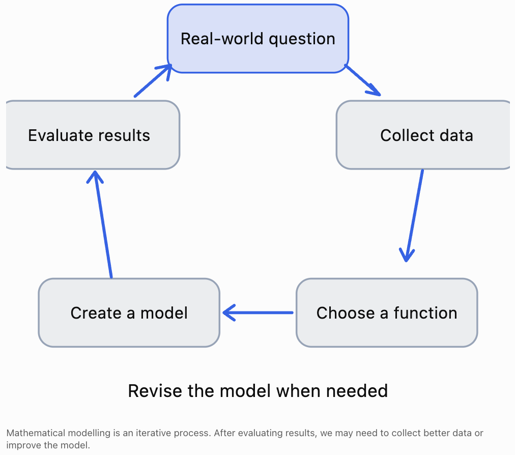
A typical modelling project follows these stages:
-
Identify a real-world question.
-
Decide which variables to investigate.
-
Collect reliable data.
-
Organise the data in tables and graphs.
-
Identify patterns.
-
Select an appropriate function.
-
Construct an equation.
-
Compare the model with the observed data.
-
Interpret results and make predictions.
-
Communicate findings and evaluate limitations.
The process is not always completed in a straight line.
For example, after plotting the data, we may realise that the original measurements were insufficient or that another function would describe the situation more accurately.
Revising a model is a normal and important part of mathematical investigation.
Choosing a Real-World Situation
The first stage of a modelling project is selecting a situation that can be investigated mathematically.
A suitable project should involve two quantities that can be measured or calculated.
Examples include:
|
Project idea |
Independent variable |
Dependent variable |
Possible function |
|---|---|---|---|
|
Bicycle rental cost |
Time |
Cost |
Linear |
|
Plant growth |
Time |
Height |
Linear, logistic, or another growth model |
|
Cooling drink |
Time |
Temperature |
Exponential decay toward room temperature |
|
Ball thrown upward |
Time |
Height |
Quadratic |
|
Square area |
Side length |
Area |
Quadratic |
|
Savings with compound interest |
Time |
Account balance |
Exponential growth |
|
Walking at steady speed |
Time |
Distance |
Linear |
|
Sound intensity with distance |
Distance |
Intensity |
Inverse-square relationship |
|
Seasonal temperature |
Time |
Temperature |
Periodic or sinusoidal |
|
Braking distance |
Speed |
Braking distance |
Approximately quadratic under fixed conditions |
The choice of function should depend on the observed relationship, not simply on the topic.
For example, plant growth may appear approximately linear over a short period but may slow down as the plant approaches its mature size.
Identifying Variables
A mathematical model usually describes how one variable depends on another.
Independent variable
The independent variable is the input.
It is often represented by x.
Examples include:
-
Time.
-
Distance travelled.
-
Number of products sold.
-
Side length.
-
Temperature.
Dependent variable
The dependent variable is the output.
It is often represented by y or f(x).
Examples include:
-
Total cost.
-
Height.
-
Profit.
-
Area.
-
Population.
Worked Example
Suppose we investigate how the distance travelled by a toy car changes over time.
The independent variable is:
Time (seconds)
The dependent variable is:
Distance travelled (metres)
We can write:
d = f(t)
This means that distance is modelled as a function of time.
Controlled conditions
In practical investigations, other variables may influence the results.
For example, when measuring toy car motion, we should consider:
-
Whether the car moves on the same surface.
-
Whether the starting position remains the same.
-
Whether the car travels along a straight path.
-
Whether the method of measuring time is consistent.
Controlling these conditions helps make the data more reliable.
Collecting Real-World Data
Reliable data is essential for developing a useful mathematical model.
Data can be collected through:
-
Direct measurements.
-
Scientific experiments.
-
Surveys.
-
Observations.
-
Public datasets.
-
Digital sensors.
-
Simulations.
Example: Measuring the motion of a toy car
Suppose a toy car travels along a straight track.
We record its distance from the starting point at regular time intervals.
The following is an illustrative dataset, not actual experimental measurements.
|
Time (s) |
Distance (m) |
|---|---|
|
0 |
0.0 |
|
1 |
1.5 |
|
2 |
3.1 |
|
3 |
4.4 |
|
4 |
6.2 |
|
5 |
7.6 |
|
6 |
9.1 |
The data suggests that distance increases approximately linearly with time.
However, the measurements are not perfectly aligned.
This could be caused by:
-
Measurement uncertainty.
-
Small changes in speed.
-
Human reaction time.
-
Surface friction.
-
Differences in how the car was released.
Real-world data often contains variation.
A mathematical model should describe the overall trend rather than necessarily passing through every measurement.
Organising Data in Tables
A data table should be clear and easy to interpret.
A good table includes:
-
Descriptive headings.
-
Correct units.
-
Consistent numerical precision.
-
Measurements arranged logically.
-
Enough observations to identify patterns.
For example:
|
Time (s) |
Distance (m) |
|---|---|
|
0 |
0.0 |
|
1 |
1.5 |
|
2 |
3.1 |
|
3 |
4.4 |
Avoid using headings such as simply "x" and "y" in a final scientific report when meaningful variable names are available.
Instead, write:
Time (s) and Distance (m)
This makes the data understandable to someone who did not conduct the experiment.
Creating Scatter Plots
A scatter plot represents pairs of measured values on a coordinate plane.
Each point represents one observation.
For the toy car experiment:
-
Time is placed on the horizontal axis.
-
Distance is placed on the vertical axis.
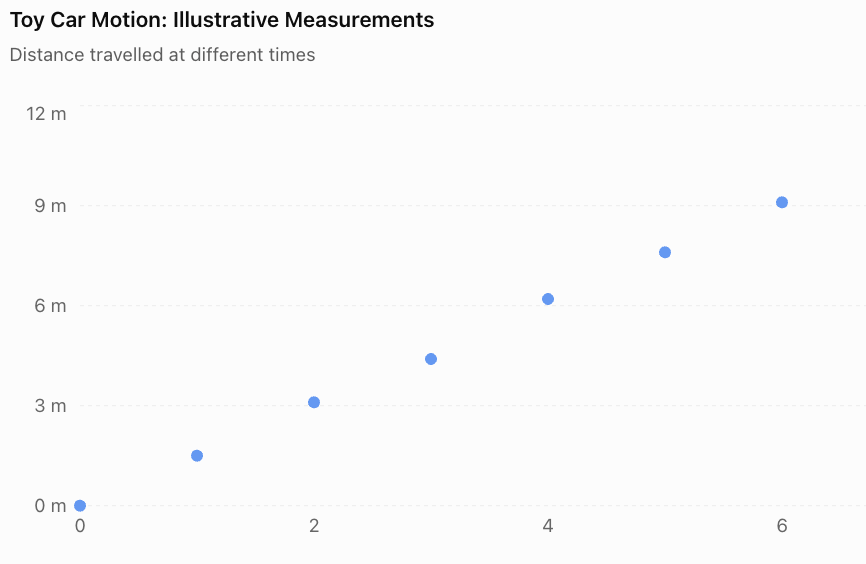
The plotted points show an upward trend.
This suggests that distance increases as time increases.
The points are also approximately arranged along a straight line.
Therefore, a linear function may be a suitable model.
Important distinction
A scatter plot shows the observed measurements.
A model graph represents the mathematical relationship used to describe those measurements.
The two should be compared, but they are not necessarily identical.
Recognising Function Patterns
One of the most important modelling skills is recognising the shape of a relationship.
Different function families produce different patterns.
Linear relationships
A linear function has the form:
y = mx + c
Its graph is a straight line.
A linear model is appropriate when the dependent variable changes by approximately the same amount for equal increases in the independent variable.
Examples include:
-
Distance travelled at constant speed.
-
Cost with a fixed fee and constant rate.
-
Earnings at a fixed hourly wage.
Quadratic relationships
A quadratic function has the form:
y = ax² + bx + c
Its graph is a parabola.
Quadratic models are useful when the rate of change changes approximately linearly with the input.
Examples include:
-
Height of a projectile under constant gravitational acceleration.
-
Area as a function of side length.
-
Some simplified profit and revenue models.
Exponential relationships
An exponential function has the form:
y = abˣ
where a ≠ 0, b > 0, and b ≠ 1.
Exponential models are useful when a quantity changes by approximately the same percentage over equal input intervals.
Examples include:
-
Compound interest.
-
Idealised population growth.
-
Radioactive decay.
-
Cooling toward a constant surrounding temperature, using a shifted exponential model.
Inverse relationships
An inverse function may have the form:
y = k/x
where x ≠ 0.
Examples include:
-
Time required to travel a fixed distance at different speeds.
-
Pressure and volume of an ideal gas at constant temperature, under suitable conditions.
Periodic relationships
Periodic functions repeat patterns over regular intervals.
Sine and cosine functions are commonly used:
y = A sin(B(x − h)) + k
Examples include:
-
Oscillations.
-
Seasonal patterns.
-
Tides.
-
Rotating machinery.
Comparing Function Families
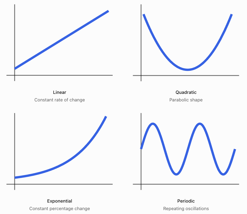
These graph shapes help us select possible models, but visual appearance alone is not enough.
We must also consider the context, mathematical assumptions, and how well the model matches the data.
Creating a Linear Model from Data
Return to the toy car measurements.
Suppose we estimate a line using two representative points:
(0, 0) and (6, 9.1)
The gradient is:
m = (y₂ − y₁)/(x₂ − x₁)
Substitute:
m = (9.1 − 0)/(6 − 0)
m ≈ 1.52
The y-intercept is approximately zero.
Therefore, a simple linear model is:
d(t) = 1.52t
where:
-
d is distance in metres.
-
t is time in seconds.
Interpreting the gradient
The gradient represents speed.
A gradient of 1.52 means the toy car travels approximately 1.52 metres per second under this model.
Making a prediction
How far will the car travel after 8 seconds?
d(8) = 1.52(8)
d(8) = 12.16
Predicted distance ≈ 12.16 m
This prediction assumes the car continues moving at approximately the same speed.
Evaluating the model
The model predicts:
Time (s)
Measured distance (m)
Predicted distance (m)
0
0.0
0.00
1
1.5
1.52
2
3.1
3.04
3
4.4
4.56
4
6.2
6.08
5
7.6
7.60
6
9.1
9.12
The predictions are reasonably close to the illustrative measurements.
This supports using a linear model over the observed interval.
However, the line was estimated from selected points rather than calculated using formal regression.
A least-squares regression line could provide a more systematic fit.
Residuals and Model Accuracy
A residual is the difference between an observed value and the value predicted by a model.
Residual = Observed value − Predicted value
Worked Example
At t = 3 seconds:
Observed distance = 4.4 m
Predicted distance = 1.52(3) = 4.56 m
Residual:
4.4 − 4.56 = −0.16 m
The negative residual means the model overestimated the observed distance by 0.16 m.
Interpreting residuals
-
Positive residual: the observed value is above the prediction.
-
Negative residual: the observed value is below the prediction.
-
Zero residual: the prediction matches the observation.
A good model generally has relatively small residuals with no strong systematic pattern.
If residuals consistently form a curve, a different function family may be more suitable.
A model with very small residuals is not automatically the best model, however. It must also make sense in the real-world situation and avoid unnecessary complexity.
Creating a Quadratic Model
Suppose we investigate the height of a ball thrown vertically upward.
Under a simplified model with constant gravitational acceleration and negligible air resistance:
h(t) = −4.9t² + v₀t + h₀
where:
-
h(t) = height in metres.
-
t = time in seconds.
-
v₀ = initial vertical velocity in metres per second.
-
h₀ = initial height in metres.
Suppose the ball is released from a height of 1.5 m with an initial upward velocity of 14.7 m/s.
Then:
h(t) = −4.9t² + 14.7t + 1.5
Finding the maximum height
The vertex occurs at:
t = −b/(2a)
Here:
a = −4.9
b = 14.7
Therefore:
t = −14.7/[2(−4.9)]
t = 1.5 s
Substitute:
h(1.5) = −4.9(1.5)² + 14.7(1.5) + 1.5
h(1.5) = −11.025 + 22.05 + 1.5
h(1.5) = 12.525
Maximum height ≈ 12.53 m
The ball reaches its maximum height after 1.5 seconds.
Finding when the ball reaches the ground
Set h(t) = 0:
0 = −4.9t² + 14.7t + 1.5
Using the quadratic formula, the positive solution is approximately:
t ≈ 3.10 s
The ball reaches the ground approximately 3.10 seconds after release.
Interpreting the model
The model predicts that:
-
The ball begins 1.5 m above the ground.
-
It rises until t = 1.5 s.
-
Its maximum height is approximately 12.53 m.
-
It then falls.
-
It reaches the ground at approximately 3.10 s.
The practical domain is approximately:
0 ≤ t ≤ 3.10
The model should not be used to predict the ball's height long after it hits the ground.
Creating an Exponential Model
Suppose a population of microorganisms starts at 200 and increases by 15% every hour.
The population can be modeled by:
P(t) = 200(1.15)ᵗ
where t is time in hours.
Understanding the equation
-
200 is the initial population.
-
1.15 is the growth factor.
-
0.15 represents a 15% increase per hour.
-
t is the number of hours.
Making predictions
After 4 hours:
P(4) = 200(1.15)⁴
P(4) ≈ 349.8
The model predicts approximately 350 microorganisms.
After 8 hours:
P(8) = 200(1.15)⁸
P(8) ≈ 611.8
The model predicts approximately 612 microorganisms.
Evaluating the model
Exponential growth may describe a population over a limited period.
However, real populations cannot increase indefinitely without constraints.
Factors such as food supply, space, competition, and waste accumulation may eventually slow growth.
Therefore, the model may be useful for short-term predictions but unsuitable for very long-term predictions.
Interpolation and Extrapolation
Models can be used to estimate values that were not directly measured.
Two important terms are interpolation and extrapolation.
Interpolation
Interpolation means estimating a value within the range of collected data.
For example, suppose we measured a car's distance between 0 and 6 seconds.
Using the model to estimate distance at 2.5 seconds is interpolation.
d(2.5) = 1.52(2.5)
d(2.5) = 3.8 m
Extrapolation
Extrapolation means predicting beyond the range of collected data.
Using the same model to estimate distance after 20 seconds is extrapolation.
d(20) = 1.52(20)
d(20) = 30.4 m
However, this prediction may be unreliable if the car slows down, changes direction, or reaches the end of the track.
Extrapolation generally requires greater caution because the relationship may change beyond the observed data.
Using Technology to Build Models
Digital tools make mathematical modelling easier.
Common options include:
-
Desmos — plotting functions and using regression tools.
-
GeoGebra — graphing, regression, and mathematical exploration.
-
Microsoft Excel — organising data, scatter plots, and trendlines.
-
Google Sheets — tables, charts, and regression calculations.
Example workflow using a spreadsheet
-
Enter the independent variable in the first column.
-
Enter the dependent variable in the second column.
-
Highlight the data.
-
Insert a scatter plot.
-
Add a trendline.
-
Choose a suitable model type.
-
Display the trendline equation when supported.
-
Compare the predicted values with the measurements.
-
Use the equation to make predictions.
Technology helps us fit models more efficiently, but we must still decide whether the model makes mathematical and practical sense.
Evaluating a Mathematical Model
A mathematical model should be evaluated rather than accepted automatically.
Useful evaluation questions include:
-
Does the model describe the observed data accurately?
-
Does the equation have a reasonable interpretation?
-
Are the units correct?
-
Does the model follow the expected scientific or mathematical relationship?
-
Are there large differences between observed and predicted values?
-
Is the model suitable for predictions outside the observed interval?
-
What assumptions were made?
-
What factors were ignored?
-
Could a different function provide a better model?
Accuracy versus usefulness
A model does not have to match every observation perfectly to be useful.
For example, a linear model may describe the motion of a toy car well enough to estimate its average speed, even if small variations occur in the measurements.
However, if the car accelerates significantly, a quadratic model may provide a better description of distance over time.
Model limitations
All mathematical models simplify reality.
Possible limitations include:
-
Measurement uncertainty.
-
Small sample sizes.
-
Uncontrolled variables.
-
Changes in environmental conditions.
-
Incorrect assumptions.
-
Limited data ranges.
-
Natural variation.
-
Instrument precision.
A strong modelling report explains these limitations rather than ignoring them.
Communicating Mathematical Findings
Mathematical modelling is not complete until the results are clearly communicated.
A good report should explain:
-
The question being investigated.
-
The data collection method.
-
The variables and their units.
-
The mathematical function selected.
-
The equation of the model.
-
The graph and important features.
-
The interpretation of coefficients.
-
Predictions made using the model.
-
Evidence supporting the model.
-
Limitations and possible improvements.
Example of mathematical communication
Suppose a student models bicycle rental cost using:
C
= 3h + 5
A weak explanation might be:
"The graph goes up and the equation works."
A stronger explanation would be:
"The relationship between rental duration and total cost is linear. The gradient of 3 represents the additional cost of $3 per hour, while the y-intercept of 5 represents the fixed rental fee. The model predicts a total cost of $17 for a four-hour rental. This model assumes that the hourly rate remains constant and that no additional charges apply."
The stronger explanation uses mathematical language and interprets the equation in context.
Student Project: Investigating a Real-World Function
Project Goal
Investigate a real-world relationship, collect or obtain data, construct a mathematical model, and evaluate how well the model describes the situation.
Project Instructions
Choose a research question
Select a situation involving two measurable variables.
Examples:
-
How does distance travelled change with time?
-
How does the height of a bouncing ball change between bounces?
-
How does the cost of a service change with usage?
-
How does the area of a square change with side length?
-
How does a hot drink's temperature change over time?
-
How does the length of a shadow change during the day?
Identify the variables
Clearly state:
-
Independent variable.
-
Dependent variable.
-
Units.
-
Relevant controlled conditions.
Collect data
Aim to collect at least 8–12 data points, where practical.
Record the data in a clear table.
If using a public dataset, identify the source.
Create a scatter plot
Label both axes with quantities and units.
Use an appropriate scale.
Choose a mathematical function
Consider whether the relationship is linear, quadratic, exponential, inverse, periodic, or another type.
Explain why the function was selected.
Construct an equation
Use calculations, graphing technology, or regression to determine a suitable equation.
Explain the meaning of the coefficients.
Analyse the model
Identify relevant features, such as:
-
Intercepts.
-
Increasing and decreasing intervals.
-
Maximum and minimum values.
-
Domain and range.
-
End behaviour.
-
Rate of change.
Not every feature will be relevant to every model.
Evaluate accuracy
Compare model predictions with observed data.
Calculate residuals for selected points.
Identify limitations.
Make predictions
Use the equation to make at least two predictions.
Include one interpolation prediction and, where reasonable, one cautious extrapolation prediction.
Communicate your findings
Present your results as a written report, infographic, or presentation, depending on the assignment requirements.
Suggested Project Report Structure
Research Question
State the relationship you are investigating.
Example:
"How does the distance travelled by a toy car change over time?"
Hypothesis
Predict the type of relationship.
Example:
"I predict that the distance travelled will increase approximately linearly with time if the toy car moves at a nearly constant speed."
Variables and Method
Identify the independent and dependent variables, equipment, and measurement procedure.
Data Table
Include all collected measurements and units.
Graph
Present a labelled scatter plot with the selected model.
Mathematical Model
State the equation and explain the coefficients.
Analysis
Discuss trends, intercepts, rates of change, extrema, and other relevant features.
Predictions
Show calculations and explain their meaning.
Evaluation
Discuss how well the model fits the data, its assumptions, and possible improvements.
Conclusion
Answer the research question using evidence from the model and observations.
Example Project Assessment Rubric
Suggested total: 20 marks
Criterion
Marks
Expectations
Data collection
4
Relevant, reliable data with appropriate units and method
Model selection
4
Suitable function chosen and justified
Equations and graphs
4
Correct equation, accurate graph, labelled axes
Interpretation and evaluation
4
Meaningful analysis, predictions, limitations
Mathematical communication
4
Clear explanations, correct terminology, logical presentation
Total
20
A high-quality project should demonstrate mathematical reasoning, not simply produce an attractive graph.
Common Mistakes
Choosing a function before examining the data
The function should be selected based on the observed pattern and the context.
Using too few data points
A small dataset may not reveal the true relationship.
Forgetting units
A gradient may represent metres per second, dollars per hour, or another meaningful quantity.
Confusing correlation with causation
Two variables changing together does not necessarily mean that one causes the other to change.
Assuming the model must pass through every point
Real measurements often contain uncertainty.
Using an equation without explaining its coefficients
A mathematical model should have a meaningful interpretation.
Making unrealistic extrapolations
A relationship observed over a short interval may not continue indefinitely.
Ignoring residuals
Large or patterned residuals may indicate that the selected function is unsuitable.
Confusing a prediction with a measurement
Predicted values come from the model; measured values come from observations.
Failing to evaluate limitations
A strong report recognises assumptions and sources of uncertainty.
Key Terms
-
Mathematical model: A mathematical representation of a real-world situation.
-
Modelling cycle: The process of developing, testing, and improving a mathematical model.
-
Independent variable: The input variable.
-
Dependent variable: The output variable.
-
Data point: A pair of measured or observed values.
-
Scatter plot: A graph displaying paired numerical observations.
-
Linear model: A model with a constant rate of change.
-
Quadratic model: A model based on a second-degree polynomial.
-
Exponential model: A model involving constant proportional growth or decay.
-
Regression: A statistical method for fitting a mathematical relationship to data.
-
Trendline: A line or curve representing the general pattern of data.
-
Residual: The difference between an observed value and a predicted value.
-
Interpolation: Estimating a value within the observed data range.
-
Extrapolation: Predicting a value outside the observed data range.
-
Domain: The set of permitted input values.
-
Range: The set of possible output values.
-
Gradient: The rate of change of a linear function.
-
Intercept: A point where a graph meets a coordinate axis.
-
Extremum: A maximum or minimum value.
-
Prediction: An estimated result obtained from a model.
-
Assumption: A condition accepted when constructing a model.
-
Limitation: A factor restricting the accuracy or usefulness of a model.
-
Validation: Checking whether a model describes observed reality adequately.
-
Mathematical communication: Explaining mathematical ideas using accurate terminology, equations, graphs, and reasoning.
Key Takeaways
-
Mathematical modelling connects functions to real-world situations.
-
A useful model begins with a clear question and relevant data.
-
Independent and dependent variables must be identified.
-
Tables and scatter plots help reveal patterns.
-
Linear functions describe approximately constant rates of change.
-
Quadratic functions can describe parabolic relationships.
-
Exponential functions describe constant proportional growth or decay.
-
The appropriate model depends on the data and context.
-
Equations allow us to calculate values and make predictions.
-
Residuals help evaluate the accuracy of a model.
-
Interpolation estimates values within the observed range.
-
Extrapolation predicts beyond the observed range and requires caution.
-
Models should be evaluated for accuracy, assumptions, and limitations.
-
Mathematical communication is essential for explaining and justifying findings.
Check Your Understanding
Recall and Understanding
1. Define mathematical modelling.
2. Explain the difference between an independent variable and a dependent variable.
3. Why is a scatter plot useful when selecting a mathematical model?
4. Explain the difference between interpolation and extrapolation.
5. What is a residual, and what does it tell us about a model?
Application
6. A taxi company charges a fixed fee of $4 plus $2.50 per kilometre. Write a linear model for the total cost and calculate the cost of a 12 km journey.
7. A population begins at 300 and grows by 10% per year. Write an exponential model and calculate the population after 3 years.
8. A ball's height is modeled by h(t) = −5t² + 20t + 2. Determine its maximum height and the time at which it occurs.
9. A linear model predicts a value of 18.5, while the observed value is 17.2. Calculate the residual and interpret it.
10. A student measures the side length and area of several squares. Which function family should they select, and why?
Analysis and Challenge
11. A dataset shows that a quantity increases by approximately 5 units every hour. Explain why a linear model may be appropriate.
12. A dataset shows that a quantity doubles every 3 hours. Explain why an exponential model may be more appropriate than a linear model.
13. A model describes a car travelling at a constant speed of 15 m/s. Explain why predicting its distance after 10 seconds is more reliable than predicting its distance after 10 hours if the original data covers only the first 20 seconds.
14. A student chooses a quadratic model because it passes through every measured data point, even though the data follows an approximately straight-line trend. Explain why this may not be the best modelling decision.
15. Design a brief mathematical modelling investigation involving a real-world relationship. Identify the research question, variables, expected function family, data collection method, and one limitation.
Answers to Check Your Understanding
1. Mathematical modelling is the process of representing real-world situations using mathematical relationships, equations, functions, tables, or graphs.
2. The independent variable is the input, while the dependent variable is the output that changes in response to the input.
3. A scatter plot reveals patterns in data and helps determine whether a linear, quadratic, exponential, or another model may be appropriate.
4. Interpolation estimates values within the range of observed data. Extrapolation predicts values outside that range.
5. A residual is the difference between an observed value and the model's prediction:
Residual = Observed − Predicted
Residuals help evaluate how accurately the model describes the data.
6.
Let d be distance in kilometres.
Cost model:
C(d) = 2.50d + 4
For 12 km:
C(12) = 2.50(12) + 4
C(12) = 30 + 4
Total cost = $34
7.
Initial population = 300
Growth factor = 1.10
Model:
P(t) = 300(1.10)ᵗ
After 3 years:
P(3) = 300(1.10)³
P(3) = 399.3
Predicted population ≈ 399
8.
h(t) = −5t² + 20t + 2
Vertex time:
t = −20/[2(−5)]
t = 2
Calculate:
h(2) = −5(2)² + 20(2) + 2
h(2) = −20 + 40 + 2
h(2) = 22
Maximum height = 22 m at t = 2 s
9.
Residual = Observed − Predicted
Residual = 17.2 − 18.5
Residual = −1.3
The model overestimated the observed value by 1.3 units.
10.
A quadratic model is appropriate because the area of a square is:
A = s²
where s is side length.
The relationship between side length and area is quadratic.
11.
A linear model is appropriate because the quantity changes by approximately the same amount for each equal increase in time.
This suggests a constant rate of change.
12.
An exponential model is appropriate because doubling over equal time intervals represents constant proportional growth.
A linear model would increase by a constant amount rather than a constant factor.
13.
A prediction after 10 seconds lies within the observed interval and is interpolation.
A prediction after 10 hours extends far beyond the observed interval and is extrapolation.
The car may change speed, stop, or change direction over such a long period.
Therefore, the 10-hour prediction is much less reliable.
14.
A model that passes through every measured point may be unnecessarily complicated or may fit measurement noise rather than the underlying relationship.
If the data follows an approximately straight-line trend, a linear model may be simpler, easier to interpret, and more appropriate for predictions.
15. Example investigation
Research question:
"How does the temperature of a hot drink change over time?"
Independent variable:
Time in minutes.
Dependent variable:
Temperature in °C.
Expected function family:
Exponential decay toward room temperature.
Data collection:
Measure the temperature every two minutes for 30 minutes using a thermometer.
Possible limitation:
The cooling rate may change because of air movement, the container, evaporation, or changes in surrounding temperature.
A suitable model could take the form:
T(t) = Tₐ + (T₀ − Tₐ)e^(−kt)
where:
-
Tₐ = surrounding temperature.
-
T₀ = initial temperature.
-
k = positive cooling constant.
-
t = time.
The parameters could be estimated from the measurements.
Final Summary
Mathematical modelling is a powerful method for connecting classroom mathematics with real-world problems.
By collecting data, identifying patterns, selecting suitable functions, constructing equations, and evaluating predictions, we can use mathematics to understand relationships and make informed decisions.
A successful modelling project requires more than finding an equation. It also requires explaining why the model is appropriate, interpreting its features, recognising limitations, and communicating conclusions clearly.
The most important goal of mathematical modelling is not simply to produce an equation, but to use mathematics to explain and understand a real-world situation.
-