Analyzing and Interpreting Graphs
2. Increasing and Decreasing Functions
Learning outcomes
- I can identify increasing intervals.
- I can identify decreasing intervals.
- I can compare function behavior.
- I can interpret changes in graphs.
- I can describe function trends.
Introduction
Graphs show more than the relationship between two variables. They also reveal how a quantity changes as its input increases.
For example, imagine tracking the height of a ball thrown into the air.
-
At first, the ball moves upward, so its height increases.
-
At its highest point, its height stops increasing.
-
As the ball falls, its height decreases.
These changes can be described mathematically using increasing and decreasing functions.
Understanding where a function increases or decreases allows us to identify trends, compare graphs, locate maximum and minimum values, and interpret real-world data.
This is useful in many subjects:
-
Physics: Describing changes in height, speed, and energy.
-
Biology: Studying population growth and decline.
-
Economics: Analysing changes in profit, revenue, and costs.
-
Chemistry: Investigating how concentrations change during reactions.
-
Environmental science: Interpreting changes in temperature and other measurements.
What Is an Increasing Function?
A function is increasing over an interval when its output increases as its input increases.
In simple terms:
As x increases, y increases.
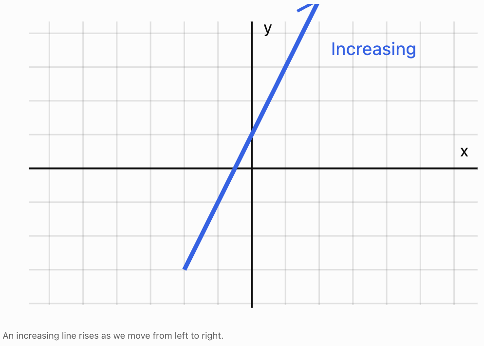
Imagine moving from left to right along a graph. If the graph rises, the function is increasing.
Example: A linear function
Consider:
y = 2x + 1
Calculate some values:
|
x |
y |
|---|---|
|
−2 |
−3 |
|
−1 |
−1 |
|
0 |
1 |
|
1 |
3 |
|
2 |
5 |
As x increases from −2 to 2, y increases from −3 to 5.
Therefore, the function is increasing over its entire domain.
Mathematical definition
A function f is strictly increasing on an interval if, whenever x₁ < x₂ in that interval:
f(x₁) < f(x₂)
This means a larger input always gives a larger output.
For example:
If x₁ = 1 and x₂ = 3, then for f(x) = 2x + 1:
f(1) = 3
f(3) = 7
Since 1 < 3 and 3 < 7, these values are consistent with an increasing function.
One pair of values alone does not prove that a function is increasing over an entire interval, but it helps illustrate the idea.
What Is a Decreasing Function?
A function is decreasing over an interval when its output decreases as its input increases.
In simple terms:
As x increases, y decreases.
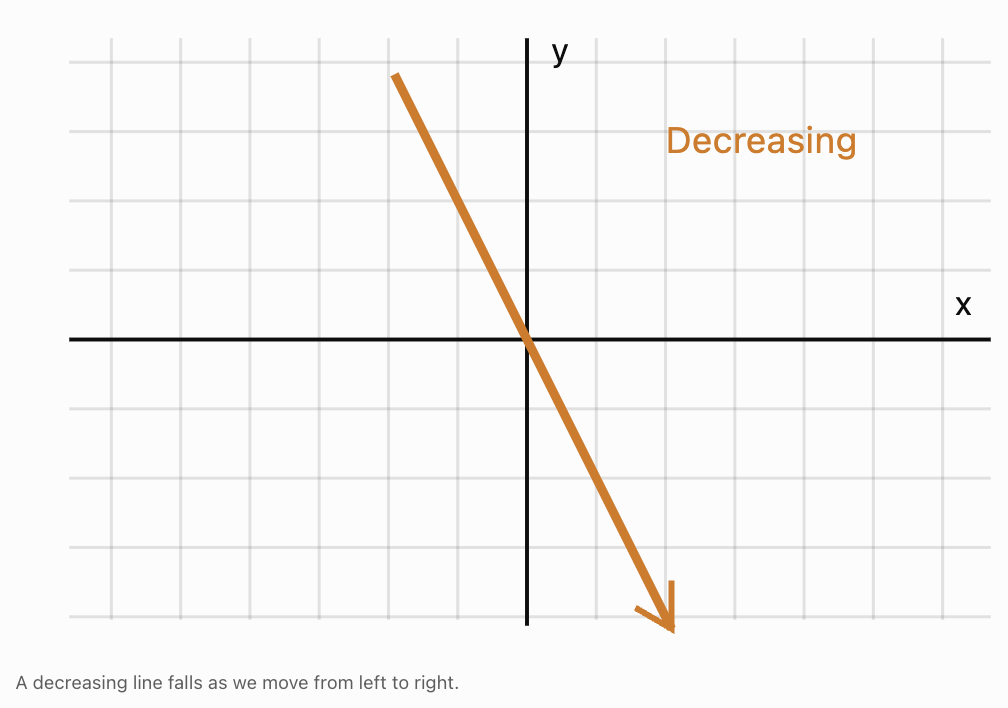
When moving from left to right along a graph, a decreasing function falls.
Example: A linear function
Consider:
y = −3x + 4
|
x |
y |
|---|---|
|
−2 |
10 |
|
−1 |
7 |
|
0 |
4 |
|
1 |
1 |
|
2 |
−2 |
As x increases, y decreases.
Therefore, the function is decreasing over its entire domain.
Mathematical definition
A function f is strictly decreasing on an interval if, whenever x₁ < x₂:
f(x₁) > f(x₂)
This means a larger input always gives a smaller output.
Constant Functions
Not every function is increasing or decreasing.
Consider:
y = 5
Regardless of the value of x, the output remains 5.
|
x |
y |
|---|---|
|
−2 |
5 |
|
−1 |
5 |
|
0 |
5 |
|
1 |
5 |
|
2 |
5 |
The graph is a horizontal line.
It is constant over its entire domain.
In strict terminology, a constant function is neither strictly increasing nor strictly decreasing.
Some textbooks also use non-decreasing and non-increasing:
-
Non-decreasing means outputs never go down as x increases.
-
Non-increasing means outputs never go up as x increases.
Under these broader definitions, a constant function is both non-decreasing and non-increasing.
For these notes, increasing and decreasing will generally mean strictly increasing and decreasing unless stated otherwise.
Understanding Intervals
Many functions are not increasing or decreasing everywhere.
Instead, their behaviour changes over different parts of their domains.
An interval is a continuous section of the x-axis.
For example:
−3 < x < 2
describes all x-values between −3 and 2.
In interval notation, this is written:
(−3, 2)
The parentheses indicate that the endpoints are not included.
Common interval notation
|
Notation |
Meaning |
|---|---|
|
(a, b) |
Between a and b, excluding both endpoints |
|
[a, b] |
Between a and b, including both endpoints |
|
(−∞, a) |
All values less than a |
|
(a, ∞) |
All values greater than a |
|
(−∞, ∞) |
All real numbers |
Infinity always uses parentheses because it is not a real endpoint.
Why interval notation matters
A function may increase over one interval and decrease over another.
We need a precise way to describe where each behaviour occurs.
Identifying Increasing and Decreasing Intervals from Graphs
To identify intervals:
-
Read the graph from left to right.
-
Identify sections where the graph rises.
-
Identify sections where the graph falls.
-
Locate any turning points.
-
Record the corresponding x-values using interval notation.
Worked Example: A quadratic function
Consider:
f(x) = x²
The graph is a U-shaped parabola with vertex at (0, 0).
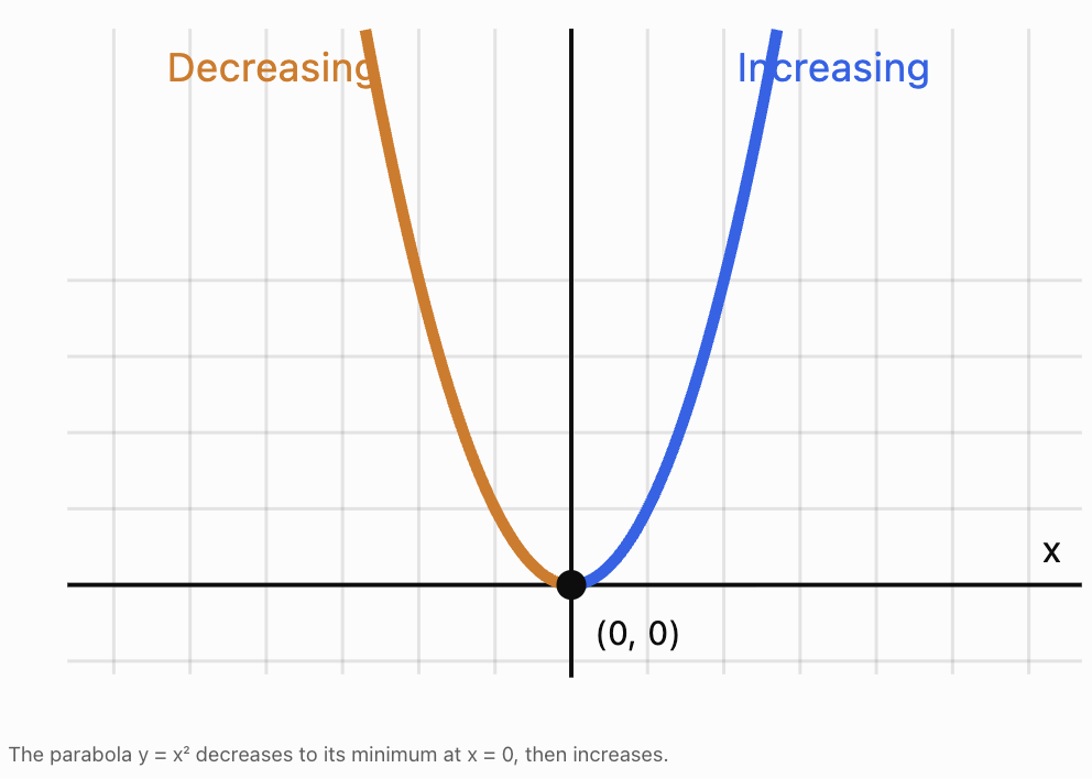
On the left side of the vertex, the graph falls as x increases.
On the right side, the graph rises.
Therefore:
Decreasing interval: (−∞, 0)
Increasing interval: (0, ∞)
The vertex at x = 0 is a turning point where the direction changes.
We usually use open intervals when reporting increasing and decreasing behaviour so that turning points clearly separate the intervals. For continuous functions, including the turning-point endpoint can also be mathematically valid when describing monotonicity on a closed or half-closed interval.
Increasing and Decreasing Quadratic Functions
The direction of a quadratic function depends on whether its parabola opens upward or downward.
The vertex is particularly important because it separates the increasing and decreasing intervals.
Upward-opening parabolas
Consider:
f(x) = (x − 3)² + 2
The vertex is:
(3, 2)
The graph opens upward, so it decreases until x = 3 and then increases.
-
Decreasing: (−∞, 3)
-
Increasing: (3, ∞)
-
Minimum value: 2
Downward-opening parabolas
Consider:
g(x) = −2(x + 1)² + 8
The vertex is:
(−1, 8)
The graph opens downward, so it increases until x = −1 and then decreases.
-
Increasing: (−∞, −1)
-
Decreasing: (−1, ∞)
-
Maximum value: 8
Comparing the two types
|
Feature |
Opens upward |
Opens downward |
|---|---|---|
|
Quadratic coefficient |
Positive |
Negative |
|
Left of vertex |
Decreasing |
Increasing |
|
Right of vertex |
Increasing |
Decreasing |
|
Vertex represents |
Minimum |
Maximum |
Worked Example: Finding intervals from standard form
Consider:
f(x) = 2x² − 8x + 5
The x-coordinate of the vertex is:
x = −b/(2a)
Here:
a = 2, b = −8
Substitute:
x = −(−8)/(2 × 2)
x = 8/4
x = 2
Because a is positive, the parabola opens upward.
Therefore:
Decreasing: (−∞, 2)
Increasing: (2, ∞)
To calculate the minimum:
f(2) = 2(2)² − 8(2) + 5
f(2) = 8 − 16 + 5
f(2) = −3
The minimum occurs at:
(2, −3)
Increasing and Decreasing Linear Functions
For a linear function:
y = mx + c
the gradient m determines its behaviour.
-
If m > 0, the function is increasing.
-
If m < 0, the function is decreasing.
-
If m = 0, the function is constant.
Worked Example
Compare:
A: y = 4x + 2
B: y = −2x + 7
C: y = 5
Function A has gradient 4, so it is increasing everywhere.
Function B has gradient −2, so it is decreasing everywhere.
Function C has gradient 0, so it is constant everywhere.
Both A and B have domains consisting of all real numbers.
Therefore:
-
A is increasing on (−∞, ∞).
-
B is decreasing on (−∞, ∞).
-
C is constant on (−∞, ∞).
Comparing rates of change
Consider:
f(x) = 2x + 1
g(x) = 5x + 1
Both functions are increasing.
However, g(x) increases more rapidly because its gradient is larger.
For each increase of 1 in x:
-
f(x) increases by 2.
-
g(x) increases by 5.
A function can therefore be increasing without increasing at the same rate as another function.
Increasing and Decreasing Absolute Value Functions
Consider the parent function:
f(x) = |x|
Its graph has a V shape.
The vertex is (0, 0).
To the left of the vertex, the function decreases.
To the right, it increases.
Therefore:
-
Decreasing: (−∞, 0)
-
Increasing: (0, ∞)
Worked Example: Transformed absolute value function
Consider:
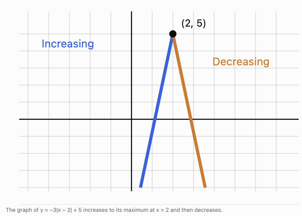
g(x) = −3|x − 2| + 5
The vertex is:
(2, 5)
The negative coefficient reflects the graph across the x-axis.
It becomes an upside-down V.
Therefore:
Increasing: (−∞, 2)
Decreasing: (2, ∞)
The function has a maximum value of 5.
Increasing and Decreasing Exponential Functions
Exponential functions are often used to model growth and decay.
Consider:
f(x) = 2ˣ
As x increases, the output increases.
For example:
|
x |
2ˣ |
|---|---|
|
−2 |
0.25 |
|
−1 |
0.5 |
|
0 |
1 |
|
1 |
2 |
|
2 |
4 |
The function is increasing on:
(−∞, ∞)
Now consider:
g(x) = (1/2)ˣ
|
x |
(1/2)ˣ |
|---|---|
|
−2 |
4 |
|
−1 |
2 |
|
0 |
1 |
|
1 |
0.5 |
|
2 |
0.25 |
The function is decreasing on:
(−∞, ∞)
General rule
For:
y = bˣ
where b > 0 and b ≠ 1:
-
If b > 1, the function is increasing.
-
If 0 < b < 1, the function is decreasing.
A vertical reflection can reverse these trends.
For example:
y = −2ˣ
is decreasing because it is the reflection of an increasing exponential function across the x-axis.
Functions with Several Increasing and Decreasing Intervals
Some functions change direction more than once.
Consider:
f(x) = x³ − 3x
This cubic function has two turning points.
The turning points are:
-
A local maximum at (−1, 2).
-
A local minimum at (1, −2).
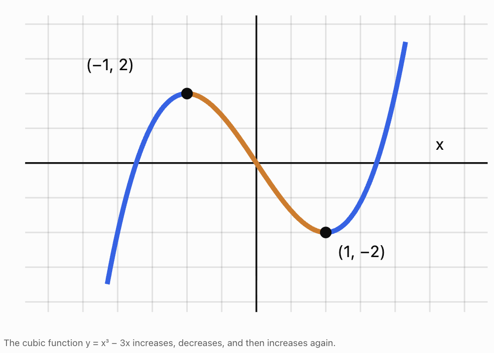
Read the graph from left to right:
-
It rises until x = −1.
-
It falls between x = −1 and x = 1.
-
It rises again after x = 1.
Therefore:
Increasing: (−∞, −1) and (1, ∞)
Decreasing: (−1, 1)
A function can have several separate increasing intervals.
We list these intervals individually rather than combining them into one interval that includes decreasing behaviour.
Using Tables to Identify Trends
Sometimes we have a table rather than a graph.
Consider:
|
Time |
Temperature (°C) |
|---|---|
|
8 |
18 |
|
9 |
21 |
|
10 |
24 |
|
11 |
26 |
|
12 |
26 |
|
13 |
25 |
|
14 |
23 |
From the table:
-
Temperature rises from 8:00 to 11:00.
-
Temperature stays unchanged between 11:00 and 12:00.
-
Temperature falls from 12:00 to 14:00.
We can describe the observed trend as:
Increasing: 8:00–11:00
Constant: 11:00–12:00
Decreasing: 12:00–14:00
However, a table only shows measured values.
Without additional information, we cannot be certain that the temperature increased continuously between every pair of measurements.
A graph or mathematical model can help estimate the behaviour between observations.
Comparing Function Behaviour
When comparing two functions, we can investigate more than whether they are increasing or decreasing.
We can also compare how rapidly their outputs change.
Example: Two increasing linear functions
Consider:
f(x) = 2x + 1
g(x) = 5x − 3
Both functions are increasing over all real numbers.
However, their gradients differ.
-
f(x) increases by 2 units for every increase of 1 in x.
-
g(x) increases by 5 units for every increase of 1 in x.
Therefore, g(x) increases more rapidly.
Example: Linear versus exponential growth
Consider:
f(x) = 2x + 1
g(x) = 2ˣ
Both functions are increasing.
However, their rates of change behave differently.
|
x |
f(x) = 2x + 1 |
g(x) = 2ˣ |
|---|---|---|
|
0 |
1 |
1 |
|
1 |
3 |
2 |
|
2 |
5 |
4 |
|
3 |
7 |
8 |
|
4 |
9 |
16 |
|
5 |
11 |
32 |
The linear function increases by a constant amount.
The exponential function increases by a constant percentage, so its absolute increases become larger.
At first, the linear function is larger.
Later, the exponential function becomes much larger.
Two functions can both be increasing while having very different long-term behaviour.
Average Rate of Change
The average rate of change measures how much a function's output changes per unit increase in its input over an interval.
For a function f(x), between x = a and x = b:
Average rate of change = [f(b) − f(a)]/(b − a)
where a ≠ b.
This is the gradient of the secant line joining the two points on the graph.
Worked Example
Consider:
f(x) = x²
Find the average rate of change between x = 1 and x = 3.
First calculate:
f(1) = 1
f(3) = 9
Then:
Average rate of change = (9 − 1)/(3 − 1)
= 8/2
= 4
Over this interval, the output increases by an average of 4 units for each increase of 1 in x.
Positive and negative average rates
-
A positive average rate means the output at the end is greater than at the start.
-
A negative average rate means the output at the end is smaller than at the start.
-
A zero average rate means the endpoint outputs are equal.
However, a positive average rate does not prove that the function increases throughout the interval.
For example, a graph could rise, fall, and then rise again while still ending higher than it started.
Local Maximum and Minimum Points
An increasing function may eventually stop increasing and begin decreasing.
The point where this happens is often a local maximum.
Similarly, a function may stop decreasing and begin increasing.
This point is often a local minimum.
Local maximum
A local maximum occurs when a function has a value greater than or equal to nearby function values.
For example:
f(x) = −(x − 2)² + 5
The graph increases until x = 2, then decreases.
The vertex (2, 5) is a local maximum.
It is also the absolute maximum of this function.
Local minimum
A local minimum occurs when a function has a value less than or equal to nearby function values.
For example:
g(x) = (x + 3)² − 4
The graph decreases until x = −3, then increases.
The vertex (−3, −4) is a local minimum.
It is also the absolute minimum.
Local versus absolute extrema
A local maximum is higher than nearby values.
An absolute maximum is the greatest value over the entire domain being considered.
Similarly, a local minimum is lower than nearby values, while an absolute minimum is the smallest value over the domain.
A function can have several local maxima and minima without having an absolute maximum or minimum.
How Transformations Affect Increasing and Decreasing Intervals
Graph transformations can change the intervals over which a function increases or decreases.
Vertical translations
Consider:
f(x) = x²
g(x) = x² + 5
Both functions:
-
Decrease on (−∞, 0).
-
Increase on (0, ∞).
A vertical translation does not change where the function increases or decreases.
Horizontal translations
Consider:
f(x) = x²
g(x) = (x − 4)²
For f(x):
-
Decreasing: (−∞, 0)
-
Increasing: (0, ∞)
For g(x):
-
Decreasing: (−∞, 4)
-
Increasing: (4, ∞)
The horizontal translation shifts the turning point and therefore shifts the interval boundaries.
Reflection across the x-axis
Consider:
f(x) = x²
g(x) = −x²
For f(x):
-
Decreasing: (−∞, 0)
-
Increasing: (0, ∞)
For g(x):
-
Increasing: (−∞, 0)
-
Decreasing: (0, ∞)
A reflection across the x-axis reverses increasing and decreasing behaviour.
Vertical stretches and compressions
Multiplying a function by a positive number does not change its increasing or decreasing intervals.
For example:
f(x) = x²
g(x) = 5x²
Both decrease for x < 0 and increase for x > 0.
The graph becomes narrower, but the direction of change remains the same.
Real-World Application: Projectile Motion
A ball is thrown upward from a platform.
Its height is modeled by:
h(t) = −5t² + 20t + 5
where:
-
h is height in metres.
-
t is time in seconds.
Step 1: Find the turning point
The vertex occurs at:
t = −b/(2a)
Here:
a = −5, b = 20
t = −20/[2(−5)]
t = 2
Step 2: Calculate the maximum height
h(2) = −5(2)² + 20(2) + 5
h(2) = −20 + 40 + 5
h(2) = 25
Maximum height:
25 m
Step 3: Identify the intervals
The ball rises from t = 0 to t = 2.
Therefore, height is increasing on:
(0, 2)
The ball then falls until it reaches the ground.
Solve:
−5t² + 20t + 5 = 0
t = 2 + √5 ≈ 4.24 s
Therefore, over the physical flight:
Decreasing: (2, 4.24), approximately
Interpretation
The ball's height increases while it rises and decreases while it falls.
Notice that the ball is moving during both intervals.
A decreasing height does not mean the ball has stopped moving; it means its vertical position is becoming smaller.
Real-World Application: Population Changes
Suppose a population is modeled by:
P(t) = 500(1.06)ᵗ
where t is time in years.
Since the exponential base 1.06 is greater than 1, the function is increasing.
The population grows by 6% each year under the model.
Now consider:
Q(t) = 500(0.94)ᵗ
Because 0.94 is between 0 and 1, the function is decreasing.
The population declines by 6% each year.
Comparing the models
Both populations begin at 500.
However:
-
P(t) represents exponential growth.
-
Q(t) represents exponential decay.
The difference becomes greater over time.
These models could represent populations under different environmental conditions, although actual populations are affected by many factors.
Real-World Application: Business Profit
Suppose a business models profit using:
P(x) = −2(x − 30)² + 1800
where x represents hundreds of products sold.
The parabola opens downward.
Its vertex is:
(30, 1800)
Therefore, the maximum modeled profit is $1,800 when 3,000 products are sold.
Increasing interval
For x < 30, profit increases as sales increase.
Within the practical domain x ≥ 0:
Increasing: (0, 30)
Decreasing interval
For x > 30, profit decreases as sales increase.
Decreasing: (30, ∞)
The second interval describes the mathematical model, although real-world production constraints may restrict its domain.
Interpretation
Selling more products does not always increase profit under this model.
Beyond the optimal sales level, additional costs or pricing effects may reduce profitability.
Real-World Application: Temperature Trends
Consider a simplified temperature model:
T(t) = −0.5(t − 14)² + 30
where t represents the hour of the day.
The vertex is:
(14, 30)
The maximum modeled temperature is 30°C at 14:00, or 2:00 p.m.
The function:
-
Increases before 14:00.
-
Decreases after 14:00.
Over the interval 8 ≤ t ≤ 20:
Increasing: (8, 14)
Decreasing: (14, 20)
This model could represent a simplified daily temperature pattern.
Actual temperatures may fluctuate and do not necessarily follow a perfect parabola.
Describing Function Trends
When describing a graph, it is useful to go beyond simply stating that it increases or decreases.
Consider the following descriptions:
|
Trend |
Meaning |
|---|---|
|
Increasing steadily |
Output rises at a constant rate |
|
Increasing more rapidly |
Output rises at an increasing rate |
|
Increasing more slowly |
Output rises, but its rate of increase becomes smaller |
|
Decreasing steadily |
Output falls at a constant rate |
|
Decreasing more rapidly |
Output falls at an increasingly negative rate |
|
Decreasing more slowly |
Output falls, but the rate of decrease becomes smaller |
|
Constant |
Output remains unchanged |
|
Fluctuating |
Output alternates between increases and decreases |
Example: Comparing two increasing functions
Consider:
f(x) = x
g(x) = x², for x ≥ 0
Both functions are increasing.
However:
-
f(x) increases at a constant rate.
-
g(x) increases more rapidly as x becomes larger.
Example: Increasing at a decreasing rate
Consider:
h(x) = √x, for x ≥ 0
The function increases as x increases.
However, the graph becomes progressively flatter.
For example:
|
x |
√x |
|---|---|
|
0 |
0 |
|
1 |
1 |
|
4 |
2 |
|
9 |
3 |
|
16 |
4 |
The output increases by 1 each time, but increasingly large changes in x are required.
Therefore, the function is increasing at a decreasing rate.
This distinction is important when analysing growth trends.
A Step-by-Step Method for Analysing Function Behaviour
When given an unfamiliar graph, use the following approach.
Step 1: Identify the domain.
Determine which x-values are included.
Step 2: Read the graph from left to right.
Observe whether the graph rises, falls, or stays horizontal.
Step 3: Locate turning points.
Identify where the direction changes.
Step 4: Record interval boundaries.
Use the x-coordinates of turning points and domain endpoints.
Step 5: Write increasing and decreasing intervals.
Use interval notation.
Step 6: Identify maximum and minimum values.
Determine whether turning points represent local or absolute extrema.
Step 7: Describe the trend in context.
Explain what increasing or decreasing means for the quantities being measured.
Step 8: Compare rates of change when appropriate.
Determine whether the function changes steadily, more rapidly, or more slowly.
Common Mistakes
Reading a graph from right to left
Increasing and decreasing intervals are determined by moving from left to right, in the direction of increasing x.
Confusing positive values with increasing functions
A function can have positive outputs while decreasing.
For example, y = 10 − x is decreasing even when y is positive.
Confusing negative values with decreasing functions
A function can have negative outputs while increasing.
For example, y = x − 10 is increasing everywhere.
Using y-values instead of x-values in interval notation
Increasing and decreasing intervals are described using input values.
Ignoring turning points
A quadratic function may increase over one interval and decrease over another.
Assuming a steeper graph always means an increasing function
A steep downward line is decreasing.
Steepness and direction are different properties.
Confusing decreasing with decreasing more rapidly
A function can decrease while becoming flatter, meaning its rate of decrease is slowing.
Assuming a positive average rate proves a function is increasing throughout
Average rate of change only compares the endpoints.
Ignoring the practical domain
A mathematical model may be defined beyond the time or quantity relevant to the real situation.
Assuming a stationary point must be a maximum or minimum
For example, y = x³ has a horizontal tangent at x = 0 but continues increasing through that point.
Key Terms
-
Increasing function: A function whose outputs rise as inputs increase.
-
Decreasing function: A function whose outputs fall as inputs increase.
-
Strictly increasing: Larger inputs always produce larger outputs within an interval.
-
Strictly decreasing: Larger inputs always produce smaller outputs within an interval.
-
Constant function: A function whose output remains unchanged.
-
Interval: A continuous set of input values.
-
Interval notation: A method of representing sets of values using brackets or parentheses.
-
Turning point: A point where a graph changes from increasing to decreasing or vice versa.
-
Local maximum: A function value greater than or equal to nearby values.
-
Local minimum: A function value less than or equal to nearby values.
-
Absolute maximum: The greatest output over a specified domain.
-
Absolute minimum: The smallest output over a specified domain.
-
Gradient: The rate of change of a straight-line graph.
-
Average rate of change: The change in output divided by the change in input over an interval.
-
Monotonic function: A function that is consistently non-decreasing or non-increasing over an interval.
-
Exponential growth: Growth by a constant percentage over equal input intervals.
-
Exponential decay: Decline by a constant percentage over equal input intervals.
-
Trend: The general direction or pattern of change in a graph or dataset.
-
Domain: The set of permitted input values.
-
Range: The set of possible output values.
Key Takeaways
-
A function is increasing when its outputs rise as x increases.
-
A function is decreasing when its outputs fall as x increases.
-
Increasing and decreasing intervals are identified by reading graphs from left to right.
-
Intervals are written using x-values, not y-values.
-
Linear functions with positive gradients are increasing.
-
Linear functions with negative gradients are decreasing.
-
Upward-opening parabolas decrease before their vertex and increase afterward.
-
Downward-opening parabolas increase before their vertex and decrease afterward.
-
Functions may have several increasing and decreasing intervals.
-
A turning point often separates intervals with different behaviour.
-
Increasing functions do not necessarily increase at constant rates.
-
Average rate of change measures the overall change between two input values.
-
Graph transformations can change increasing and decreasing intervals.
-
Understanding trends helps interpret real-world situations and make predictions.
Check Your Understanding
Recall and Understanding
1. Define an increasing function.
2. Define a decreasing function.
3. Explain how to identify increasing intervals from a graph.
4. What is the difference between a decreasing function and a constant function?
Application
5. Determine whether y = 5x − 3 is increasing or decreasing. State the interval.
6. Determine whether y = −4x + 7 is increasing or decreasing. State the interval.
7. Find the increasing and decreasing intervals of y = x² − 6x + 5.
8. Find the increasing and decreasing intervals of y = −2(x + 4)² + 9.
9. Determine the increasing and decreasing intervals of y = |x − 5|.
10. Calculate the average rate of change of f(x) = x² between x = 2 and x = 5.
Analysis and Challenge
11. Compare the behaviour of f(x) = 3x + 1 and g(x) = 7x − 2.
12. A ball's height is modeled by h(t) = −5t² + 30t + 2. Determine when its height is increasing and when it is decreasing during its flight.
13. Determine the increasing and decreasing intervals of f(x) = x³ − 12x, given that its turning points occur at x = −2 and x = 2.
14. Explain why y = √x is increasing but its rate of increase becomes smaller as x increases.
15. A business models profit using P(x) = −3(x − 20)² + 1500, where x is the number of products sold. Identify the increasing and decreasing intervals for x ≥ 0 and interpret the maximum.
Answers to Check Your Understanding
1. An increasing function has outputs that rise as its inputs increase. For a strictly increasing function, x₁ < x₂ implies f(x₁) < f(x₂).
2. A decreasing function has outputs that fall as its inputs increase. For a strictly decreasing function, x₁ < x₂ implies f(x₁) > f(x₂).
3. Read the graph from left to right. Identify sections where the graph rises and record the corresponding x-values using interval notation.
4. A decreasing function has outputs that become smaller as x increases. A constant function has outputs that remain unchanged.
5.
y = 5x − 3
Gradient = 5.
Since the gradient is positive, the function is increasing on:
(−∞, ∞)
6.
y = −4x + 7
Gradient = −4.
Since the gradient is negative, the function is decreasing on:
(−∞, ∞)
7.
y = x² − 6x + 5
a = 1, b = −6
Vertex x-coordinate:
x = −b/(2a)
x = 6/2 = 3
The parabola opens upward.
Decreasing: (−∞, 3)
Increasing: (3, ∞)
8.
y = −2(x + 4)² + 9
Vertex x-coordinate:
x = −4
The parabola opens downward.
Increasing: (−∞, −4)
Decreasing: (−4, ∞)
9.
y = |x − 5|
Vertex:
(5, 0)
The graph is V-shaped.
Decreasing: (−∞, 5)
Increasing: (5, ∞)
10.
f(x) = x²
f(2) = 4
f(5) = 25
Average rate of change:
= (25 − 4)/(5 − 2)
= 21/3
= 7
11.
f(x) = 3x + 1
g(x) = 7x − 2
Both functions are increasing on (−∞, ∞) because both gradients are positive.
However, g(x) increases more rapidly because its gradient is 7, compared with 3 for f(x).
12.
h(t) = −5t² + 30t + 2
The vertex occurs at:
t = −30/[2(−5)]
t = 3
Therefore, height increases until t = 3 seconds.
To find the landing time:
0 = −5t² + 30t + 2
5t² − 30t − 2 = 0
Using the quadratic formula:
t = [30 ± √(900 + 40)]/10
t = [30 ± √940]/10
The positive solution is approximately:
t ≈ 6.07 s
Therefore, during the physical flight:
Increasing: (0, 3)
Decreasing: (3, 6.07), approximately
13.
f(x) = x³ − 12x
The turning points occur at x = −2 and x = 2.
The function increases before x = −2, decreases between the turning points, and increases after x = 2.
Increasing: (−∞, −2) and (2, ∞)
Decreasing: (−2, 2)
14.
For y = √x, larger x-values produce larger y-values.
However, the graph becomes flatter as x increases.
For example:
-
From x = 0 to x = 1, y increases by 1.
-
From x = 1 to x = 4, y increases by 1 over 3 x-units.
-
From x = 4 to x = 9, y increases by 1 over 5 x-units.
The same increase in y requires increasingly large changes in x.
Therefore, the function is increasing at a decreasing rate.
15.
P(x) = −3(x − 20)² + 1500
The vertex is:
(20, 1500)
Because the parabola opens downward, the vertex represents a maximum.
For the practical domain x ≥ 0:
Increasing: (0, 20)
Decreasing: (20, ∞)
The maximum modeled profit is:
$1,500 when 20 products are sold.
The model suggests that increasing sales improves profit until 20 products are sold, after which further increases in sales reduce profit.
Final Summary
Increasing and decreasing functions describe how outputs change as inputs increase.
By examining graphs from left to right, identifying turning points, and using interval notation, we can determine where functions rise, fall, or remain constant.
These ideas allow us to compare function behaviour, understand maximum and minimum values, interpret rates of change, and describe trends in real-world situations.
The key distinction is between the value of a function and the direction in which that value is changing.