Transformations of Graphs

Introduction

Functions can undergo several transformations at the same time. A graph may be translated, reflected, stretched, or compressed, producing a new graph with a different position, orientation, or shape.

In earlier topics, we explored these transformations individually. However, many mathematical functions involve combinations of transformations.

For example, consider the parent function:

y = x²

Now consider:

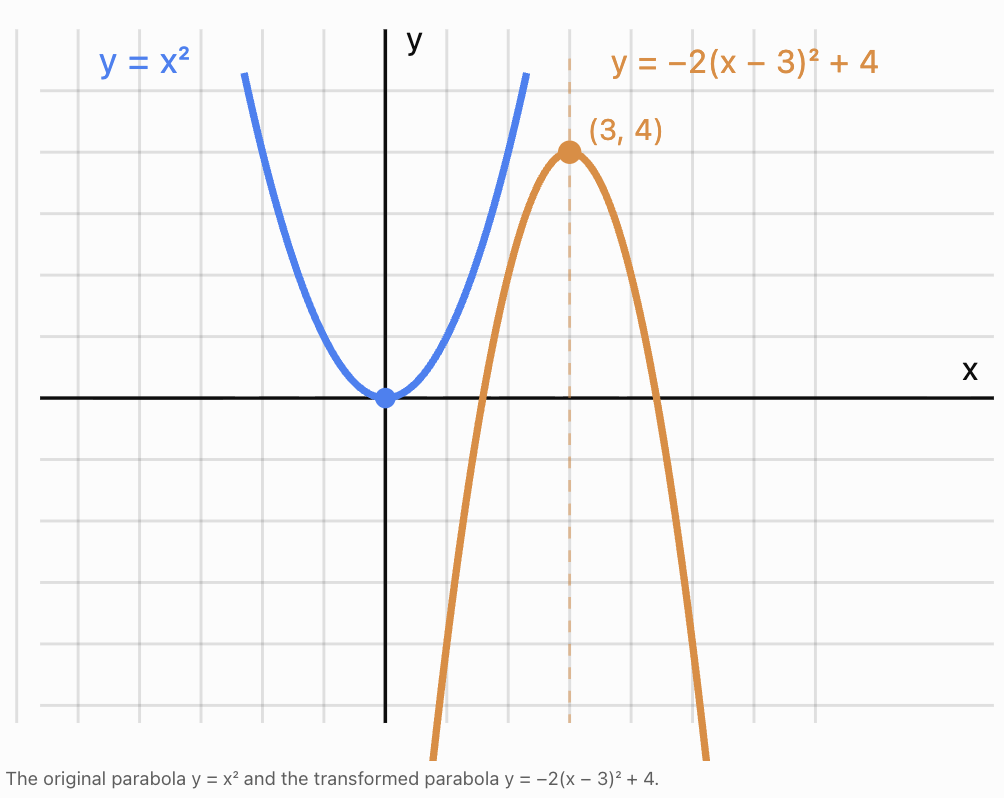
y = −2(x − 3)² + 4

This function includes several transformations:

• A horizontal translation 3 units right.

• A vertical stretch by a factor of 2.

• A reflection across the x-axis.

• A vertical translation 4 units up.

The resulting parabola opens downward, is narrower than the original, and has a vertex at (3, 4).

Understanding combined transformations allows us to interpret complicated equations, sketch graphs efficiently, and explain how different functions are related.

These skills are important when studying quadratic, absolute value, square root, exponential, and trigonometric functions, as well as mathematical models used in science and engineering.

What Are Combined Transformations?

A combined transformation occurs when two or more transformations are applied to the same graph.

The main transformations include:

• Translations: Move a graph horizontally or vertically.

• Reflections: Produce a mirror image across an axis.

• Vertical stretches: Multiply outputs by a factor greater than 1.

• Vertical compressions: Multiply outputs by a positive factor less than 1.

• Horizontal stretches: Increase horizontal distances from the y-axis.

• Horizontal compressions: Decrease horizontal distances from the y-axis.

These transformations can be combined to produce a wide variety of functions.

The challenge is recognising which transformations are present and understanding how their order affects the final graph.

General Form of Combined Transformations

A useful general form is:

g(x) = af(b(x − h)) + k

where:

• f(x) is the parent function.

• a controls vertical stretching, compression, and possible reflection across the x-axis.

• b controls horizontal stretching, compression, and possible reflection across the y-axis.

• h represents horizontal translation.

• k represents vertical translation.

The effects of the parameters are:

This form provides a systematic way to describe multiple transformations.

Understanding the Order of Transformations

The order in which transformations are applied can affect the final graph.

For example, consider:

y = x²

Suppose we want to apply:

• A vertical stretch by factor 2.

• A vertical translation 3 units up.

Method A: Stretch first, then translate

Start with:

y = x²

Stretch vertically by factor 2:

y = 2x²

Translate upward by 3:

y = 2x² + 3

Method B: Translate first, then stretch

Start with:

y = x²

Translate upward by 3:

y = x² + 3

Stretch vertically by factor 2:

y = 2(x² + 3)

y = 2x² + 6

The two final equations are different.

Therefore:

The order of transformations matters.

Important principle

When interpreting a function written in the form:

g(x) = af(b(x − h)) + k

one convenient sequence is:

1. Apply the horizontal scaling and any y-axis reflection.

2. Apply the horizontal translation.

3. Apply the vertical scaling and any x-axis reflection.

4. Apply the vertical translation.

This sequence is especially useful when transforming coordinates.

Other sequences can produce the same final graph if the translation distances are adjusted appropriately.

Coordinate Rules for Combined Transformations

Instead of transforming the entire equation repeatedly, we can transform individual points.

For:

g(x) = af(b(x − h)) + k

the coordinate rule is:

(x, y) → (x/b + h, ay + k)

provided b ≠ 0.

This rule combines horizontal scaling, horizontal translation, vertical scaling, and vertical translation.

Worked Example

Consider the transformation:

g(x) = 2f(x − 3) + 4

Here:

a = 2

b = 1

h = 3

k = 4

The coordinate rule is:

(x, y) → (x + 3, 2y + 4)

Suppose the original graph passes through:

(1, 2)

The transformed coordinates are:

x′ = 1 + 3 = 4

y′ = 2(2) + 4 = 8

Therefore:

(1, 2) → (4, 8)

The same rule applies to every point on the original graph.

Worked Example: Transforming a Parabola

Start with:

y = x²

Transform it into:

y = −2(x − 3)² + 4

Step 1: Identify the transformations

The equation contains:

• A horizontal translation 3 units right.

• A vertical stretch by factor 2.

• A reflection across the x-axis.

• A vertical translation 4 units up.

Step 2: Identify the new vertex

The original vertex is:

(0, 0)

Apply the coordinate rule:

(x, y) → (x + 3, −2y + 4)

Therefore:

(0, 0) → (3, 4)

The new vertex is:

(3, 4)

Step 3: Transform additional points

Original points on y = x²:

(−2, 4), (−1, 1), (0, 0), (1, 1), (2, 4)

Apply:

(x, y) → (x + 3, −2y + 4)

Step 4: Sketch the graph

Plot the transformed points and draw a smooth parabola.

The graph:

• Opens downward.

• Has vertex (3, 4).

• Has axis of symmetry x = 3.

• Is narrower than y = x².

• Has a maximum value of 4.

  

  Comparing Different Orders of Transformations

  Consider the parent function:

  y = |x|

  We will compare two transformation sequences.

  Sequence A: Reflect, then translate upward

  Reflect across the x-axis:

  y = −|x|

  Translate upward by 3:

  y = −|x| + 3

  The vertex is (0, 3).

  Sequence B: Translate upward, then reflect

  Translate upward by 3:

  y = |x| + 3

  Reflect across the x-axis:

  y = −(|x| + 3)

  y = −|x| − 3

  The vertex is (0, −3).

  The two graphs have different positions.

  This demonstrates that reflection and translation do not always commute.

  Two transformations commute when applying them in either order produces the same result.

  Some transformations commute, while others do not.

  For example, horizontal and vertical translations commute because they affect different coordinates.

  Combining Transformations of Absolute Value Functions

  Absolute value functions are useful for studying combined transformations because their V-shaped graphs have a clearly identifiable vertex.

  The parent function is:

  y = |x|

  Consider:

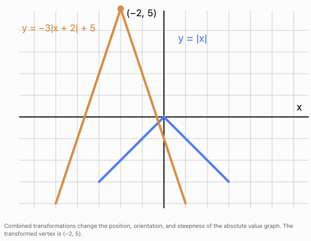
  y = −3|x + 2| + 5

  Step 1: Identify the transformations

  Compared with y = |x|:

  • Translate 2 units left.

  • Stretch vertically by a factor of 3.

  • Reflect across the x-axis.

  • Translate 5 units up.

  Step 2: Identify the vertex

  The parent vertex is (0, 0).

  The new vertex is:

  (−2, 5)

  Because the coefficient is negative, the graph opens downward.

  Step 3: Calculate key points

  Use:

  y = −3|x + 2| + 5

  x	y
  −4	−1
  −3	2
  −2	5
  −1	2
  0	−1

  

  Combining Transformations of Square Root Functions

  Consider the parent function:

  y = √x

  Its graph starts at (0, 0) and extends rightward and upward.

  Now consider:

  y = −2√(x − 4) + 3

  Identify the transformations

  • Translate 4 units right.

  • Stretch vertically by a factor of 2.

  • Reflect across the x-axis.

  • Translate 3 units up.

  Determine the starting point

  The original starting point is (0, 0).

  Using the coordinate rule:

  (x, y) → (x + 4, −2y + 3)

  The new starting point is:

  (4, 3)

  Transform other points

  Original point	Transformed point
  (0, 0)	(4, 3)
  (1, 1)	(5, 1)
  (4, 2)	(8, −1)
  (9, 3)	(13, −3)

  Domain and range

  For the square root to be defined:

  x − 4 ≥ 0

  Therefore:

  Domain: x ≥ 4

  Because the square root is non-negative and multiplied by −2:

  −2√(x − 4) ≤ 0

  Adding 3:

  Range: y ≤ 3

  The transformed graph starts at (4, 3) and curves downward to the right.

  Combining Horizontal and Vertical Scaling

  When a function contains coefficients both inside and outside its expression, we must distinguish horizontal and vertical scaling.

  Consider:

  g(x) = 2f(3x)

  The transformations are:

  • Horizontal compression by a factor of 1/3.

  • Vertical stretch by a factor of 2.

  The coordinate rule is:

  (x, y) → (x/3, 2y)

  For example, if the original function contains the point (6, 4), the transformed point is:

  (6/3, 2 × 4)

  (2, 8)

  Worked Example: Including translations

  Consider:

  g(x) = 3f(2(x − 4)) − 5

  Identify the parameters:

  a = 3

  b = 2

  h = 4

  k = −5

  Therefore:

  • Horizontal compression by a factor of 1/2.

  • Translation 4 units right.

  • Vertical stretch by a factor of 3.

  • Translation 5 units down.

  Coordinate rule:

  (x, y) → (x/2 + 4, 3y − 5)

  If the parent function contains the point (2, 3):

  x′ = 2/2 + 4 = 5

  y′ = 3(3) − 5 = 4

  The transformed point is:

  (5, 4)

  Why brackets matter

  Compare:

  g(x) = f(2(x − 4))

  and:

  g(x) = f(2x − 4)

  The first can be read as a horizontal compression by 1/2 followed by a translation 4 units right.

  The second can be rewritten as:

  g(x) = f(2(x − 2))

  It represents a horizontal compression by 1/2 followed by a translation 2 units right.

  The two equations do not describe the same transformation.

  Always factor the coefficient inside the function before identifying the horizontal translation.

  Combining Transformations of Exponential Functions

  Consider the parent function:

  y = 2ˣ

  Now consider:

  y = −3(2⁽ˣ ⁻ ²⁾) + 4

  Identify the transformations

  • Translate 2 units right.

  • Stretch vertically by a factor of 3.

  • Reflect across the x-axis.

  • Translate 4 units up.

  Transform key points

  The original function passes through:

  (0, 1), (1, 2), (2, 4)

  Apply:

  (x, y) → (x + 2, −3y + 4)

  Original point	Transformed point
  (0, 1)	(2, 1)
  (1, 2)	(3, −2)
  (2, 4)	(4, −8)

  Determine the asymptote

  The original horizontal asymptote is:

  y = 0

  The vertical stretch and reflection leave this asymptote at y = 0.

  The upward translation moves it to:

  y = 4

  The transformed graph approaches y = 4 from below.

  Its domain is all real numbers, and its range is:

  y < 4

  Combining Transformations of Trigonometric Functions

  Trigonometric functions often involve several transformations.

  Consider:

  y = 3 sin(2(x − π/4)) + 1

  Compared with y = sin x:

  • Vertical stretch by a factor of 3.

  • Horizontal compression by a factor of 1/2.

  • Translation π/4 units right.

  • Translation 1 unit up.

  The amplitude is:

  3

  The period is:

  2π/2 = π

  The midline is:

  y = 1

  The maximum value is:

  1 + 3 = 4

  The minimum value is:

  1 − 3 = −2

  7.7: Modeling with Trigonometric Functions - Mathematics LibreTexts

   

   

   

  These combined transformations are important in modeling sound waves, alternating electrical currents, vibrations, and periodic motion.

  Identifying Transformations from Equations

  A useful strategy is to compare the transformed equation with a familiar parent function.

  Example A

  y = 4(x + 3)² − 2

  Compared with y = x²:

  • Vertical stretch by factor 4.

  • Translation 3 units left.

  • Translation 2 units down.

  Example B

  y = −0.5|x − 6| + 1

  Compared with y = |x|:

  • Vertical compression by factor 0.5.

  • Reflection across the x-axis.

  • Translation 6 units right.

  • Translation 1 unit up.

  Example C

  y = √(2(x + 1)) − 4

  Compared with y = √x:

  • Horizontal compression by factor 1/2.

  • Translation 1 unit left.

  • Translation 4 units down.

  Example D

  y = −2f(−3(x − 5)) + 7

  Compared with y = f(x):

  • Horizontal compression by factor 1/3.

  • Reflection across the y-axis.

  • Translation 5 units right.

  • Vertical stretch by factor 2.

  • Reflection across the x-axis.

  • Translation 7 units up.

  The corresponding coordinate rule is:

  (x, y) → (−x/3 + 5, −2y + 7)

  Comparing Multiple Transformed Graphs

  Consider these three functions:

  A: y = (x − 2)² + 3

  B: y = 2(x − 2)² + 3

  C: y = −0.5(x − 2)² + 3

  All three have the same vertex:

  (2, 3)

  However, their shapes differ.

  Feature	Graph A	Graph B	Graph C
  Vertex	(2, 3)	(2, 3)	(2, 3)
  Opens	Upward	Upward	Downward
  Vertical scale	1	2	0.5
  Width	Standard	Narrower	Wider
  Extreme value	Minimum 3	Minimum 3	Maximum 3
  Axis of symmetry	x = 2	x = 2	x = 2

  This comparison shows how coefficients can change graph shape and orientation while leaving the vertex unchanged.

  Sketching Combined Transformations

  A reliable method for sketching transformed functions is to use key points from the parent graph.

  Step 1: Identify the parent function

  For example:

  y = x²

  Step 2: Identify the transformation parameters

  Suppose:

  y = −0.5(x + 2)² + 3

  Then:

  a = −0.5

  h = −2

  k = 3

  Step 3: Write the coordinate rule

  (x, y) → (x − 2, −0.5y + 3)

  Step 4: Select key points

  For y = x²:

  (−2, 4), (−1, 1), (0, 0), (1, 1), (2, 4)

  Step 5: Transform the points

  Original	Transformed
  (−2, 4)	(−4, 1)
  (−1, 1)	(−3, 2.5)
  (0, 0)	(−2, 3)
  (1, 1)	(−1, 2.5)
  (2, 4)	(0, 1)

  Step 6: Draw and label the graph

  The graph is a downward-opening parabola with:

  • Vertex (−2, 3).

  • Axis of symmetry x = −2.

  • Maximum value 3.

  • A wider shape than y = x².

  Step 7: Verify the sketch

  Substitute a few plotted x-values into the equation to confirm their y-values.

  Determining an Equation from a Graph

  Sometimes we are given the final graph and must work backwards to identify its equation.

  Worked Example: Quadratic graph

  A parabola has:

  • Vertex (3, −2).

  • Opens downward.

  • Passes through (4, −5).

  Assume it has the form:

  y = a(x − h)² + k

  The vertex gives:

  h = 3

  k = −2

  Therefore:

  y = a(x − 3)² − 2

  Use the point (4, −5):

  −5 = a(4 − 3)² − 2

  −5 = a − 2

  a = −3

  The equation is:

  y = −3(x − 3)² − 2

  Compared with y = x², this graph has:

  • Vertical stretch by factor 3.

  • Reflection across the x-axis.

  • Translation 3 units right.

  • Translation 2 units down.

  Verification

  At x = 4:

  y = −3(1)² − 2

  y = −5 ✓

  Applications of Combined Transformations

  Physics: Projectile motion

  The height of a projectile may be modeled by:

  h(t) = −5(t − 2)² + 25

  This is a transformed quadratic function.

  Compared with y = x²:

  • Vertical stretch by factor 5.

  • Reflection across the x-axis.

  • Translation 2 units right.

  • Translation 25 units up.

  The vertex is:

  (2, 25)

  This means the projectile reaches a maximum height of 25 m after 2 seconds.

  The equation can also be expanded:

  h(t) = −5(t² − 4t + 4) + 25

  h(t) = −5t² + 20t + 5

  The initial height is 5 m.

  Curso Multimedia y web 2.0: MOVIMIENTO PARABOLICO

   

   

   

  Business: Revenue modeling

  Suppose a company's revenue is modeled by:

  R(x) = −2(x − 50)² + 5000

  This parabola opens downward.

  Its maximum occurs at:

  x = 50

  The maximum revenue is:

  R = 5000

  The vertex form makes it easy to identify the maximum without expanding the equation.

  The vertical stretch factor determines how rapidly revenue decreases as x moves away from the optimal value.

  Biology: Periodic measurements

  Suppose a periodic biological measurement is modeled by:

  P(t) = 5 sin(2(t − 1)) + 12

  This model includes:

  • Vertical stretch by factor 5.

  • Horizontal compression by factor 1/2.

  • Translation 1 unit right.

  • Translation 12 units up.

  The amplitude is 5.

  The midline is 12.

  The period is π time units.

  The model's maximum value is 17, and its minimum value is 7.

  This type of model can represent idealised rhythmic processes, although actual biological measurements may not follow perfect sine waves.

  Evaluating Transformation Descriptions

  A single transformed graph can sometimes be described using different combinations of transformations.

  For example:

  y = 4x²

  Compared with y = x², this is a vertical stretch by factor 4.

  But:

  y = (2x)² = 4x²

  Therefore, it can also be described as a horizontal compression by factor 1/2.

  Both descriptions are valid.

  Similarly, for exponential functions:

  2(2ˣ) = 2⁽ˣ ⁺ ¹⁾

  A vertical stretch by factor 2 produces the same graph as a translation 1 unit left.

  The equation and parent function must be considered together when identifying transformations.

  This is why different-looking transformation sequences can sometimes produce identical final graphs.

  Common Mistakes

  Applying transformations in the wrong order

  A vertical stretch followed by a vertical translation may produce a different result from performing the translation first.

  For example:

  2(x² + 3) = 2x² + 6

  is different from:

  2x² + 3

  Confusing horizontal translations

  In y = f(x − 4), the graph moves 4 units right, not left.

  Forgetting to factor horizontal coefficients

  For:

  y = f(3x − 6)

  rewrite the input as:

  3x − 6 = 3(x − 2)

  The horizontal translation is 2 units right, not 6 units right.

  Confusing vertical and horizontal scaling

  In y = 3f(x), outputs are multiplied by 3.

  In y = f(3x), horizontal distances are divided by 3.

  Forgetting reflections

  A negative coefficient outside a function introduces reflection across the x-axis.

  A negative coefficient multiplying the input introduces reflection across the y-axis.

  Moving the vertex without transforming other points

  Every point must follow the same coordinate transformation rule.

  Assuming all transformations change the graph visibly

  Some functions have symmetries that make particular reflections leave the graph unchanged.

  Ignoring domain and range restrictions

  A transformed square root function may have a new starting point and different domain or range.

  Confusing different but equivalent transformation descriptions

  For some function families, horizontal scaling can produce the same graph as vertical scaling.

  Failing to verify the final graph

  Check key points, intercepts, turning points, asymptotes, and domain restrictions.

  Key Terms

  • Combined transformation: Two or more transformations applied to a graph.

  • Parent function: A basic function used as the starting point for transformations.

  • Translation: A movement of a graph without changing its shape or orientation.

  • Reflection: A transformation producing a mirror image across a line.

  • Vertical stretch: Multiplying outputs by a factor greater than 1.

  • Vertical compression: Multiplying outputs by a positive factor less than 1.

  • Horizontal stretch: Increasing horizontal distances by a specified factor.

  • Horizontal compression: Decreasing horizontal distances by a specified factor.

  • Scale factor: A number describing how coordinates or distances are multiplied.

  • Coordinate transformation rule: A rule mapping original points to transformed points.

  • Vertex: A turning point of a parabola or the corner of an absolute value graph.

  • Axis of symmetry: A line dividing a graph into mirror-image halves.

  • Amplitude: The maximum displacement of a periodic function from its midline.

  • Period: The length of one complete cycle of a periodic function.

  • Midline: The central horizontal line around which a periodic function oscillates.

  • Domain: The set of permitted input values.

  • Range: The set of possible output values.

  • Asymptote: A line approached by a graph in a specified limiting direction.

  • Commutative transformations: Transformations that produce the same result when their order is reversed.

  • Equivalent transformations: Different transformation descriptions that produce the same final graph.

  Key Takeaways

  • Combined transformations involve applying several changes to the same function.

  • The general form g(x) = af(b(x − h)) + k describes vertical and horizontal scaling, reflections, and translations.

  • The coordinate rule is (x, y) → (x/b + h, ay + k), where b ≠ 0.

  • The order of transformations can affect the final graph.

  • Horizontal and vertical scaling must be distinguished carefully.

  • Factoring expressions inside a function helps identify horizontal translations correctly.

  • Negative scaling coefficients can introduce reflections.

  • Vertices, endpoints, intercepts, and asymptotes are useful for sketching transformed graphs.

  • Domain and range restrictions may change under transformations.

  • Comparing transformed graphs helps reveal the effects of individual parameters.

  • Different transformation sequences can sometimes produce the same final function.

  • Verifying key points and features helps ensure accurate graph sketches.

   

  Check Your Understanding

  Recall and Understanding

  1. What is meant by a combined transformation?

  2. Explain why the order of transformations can affect the final graph.

  3. State the coordinate transformation rule for g(x) = af(b(x − h)) + k.

  4. Explain the difference between a vertical stretch by factor 3 and a horizontal compression by factor 1/3.

  Application

  5. Describe all transformations from y = x² to:

  y = 3(x − 4)² + 2

  6. Describe all transformations from y = |x| to:

  y = −0.5|x + 3| − 2

  7. The point (2, 5) undergoes the transformation:

  (x, y) → (x + 4, −2y + 3)

  Find its new coordinates.

  8. Write the equation obtained by transforming y = x² using a vertical stretch by factor 2, a reflection across the x-axis, a translation 3 units left, and a translation 5 units up.

  9. Determine the vertex, axis of symmetry, and range of:

  y = −2(x − 1)² + 6

  10. Describe the transformations represented by:

  g(x) = 4f(2(x − 3)) − 1

  Analysis and Challenge

  11. A parabola has vertex (−2, 5), opens downward, and passes through (0, −3). Determine its equation in vertex form.

  12. A student claims that y = 2(x² + 4) and y = 2x² + 4 represent the same transformation. Explain why this is incorrect.

  13. Transform the points (−2, 4), (0, 0), and (2, 4) using:

  g(x) = −3f(2(x − 1)) + 5

  14. Compare the graphs:

  A: y = (x − 2)² + 1

  B: y = −2(x − 2)² + 1

  Describe their similarities and differences.

  15. The function y = √x is transformed into:

  y = −2√(x + 4) + 3

  Describe the transformations, state the starting point, and determine the domain and range.

  Answers to Check Your Understanding

  1. A combined transformation involves applying two or more transformations, such as translations, reflections, stretches, or compressions, to the same graph.

  2. Transformations can affect the positions of points differently depending on their order. For example, stretching a graph vertically after translating it upward also scales the translation distance, whereas stretching first and then translating does not.

  3.

  For:

  g(x) = af(b(x − h)) + k

  the coordinate rule is:

  (x, y) → (x/b + h, ay + k)

  where b ≠ 0.

  4. A vertical stretch by factor 3 multiplies y-coordinates by 3. A horizontal compression by factor 1/3 divides x-coordinates by 3. These are different transformations, although they can sometimes produce the same graph for particular functions.

  5.

  From y = x² to y = 3(x − 4)² + 2:

  • Vertical stretch by factor 3.

  • Translation 4 units right.

  • Translation 2 units up.

  Vertex: (4, 2).

  6.

  From y = |x| to y = −0.5|x + 3| − 2:

  • Vertical compression by factor 0.5.

  • Reflection across the x-axis.

  • Translation 3 units left.

  • Translation 2 units down.

  Vertex: (−3, −2).

  7.

  (x, y) → (x + 4, −2y + 3)

  For (2, 5):

  x′ = 2 + 4 = 6

  y′ = −2(5) + 3 = −7

  Answer: (6, −7)

  8.

  Start with y = x².

  Apply the stretch and reflection:

  y = −2x²

  Translate 3 units left:

  y = −2(x + 3)²

  Translate 5 units up:

  y = −2(x + 3)² + 5

  9.

  Given:

  y = −2(x − 1)² + 6

  Vertex:

  (1, 6)

  Axis of symmetry:

  x = 1

  The parabola opens downward, so its maximum value is 6.

  Range:

  y ≤ 6

  10.

  g(x) = 4f(2(x − 3)) − 1

  Transformations:

  • Horizontal compression by factor 1/2.

  • Translation 3 units right.

  • Vertical stretch by factor 4.

  • Translation 1 unit down.

  11.

  Use vertex form:

  y = a(x − h)² + k

  The vertex is (−2, 5), so:

  y = a(x + 2)² + 5

  Substitute (0, −3):

  −3 = a(0 + 2)² + 5

  −3 = 4a + 5

  4a = −8

  a = −2

  Therefore:

  y = −2(x + 2)² + 5

  Verification:

  At x = 0:

  y = −2(2²) + 5 = −3 ✓

  12.

  The equations are:

  y = 2(x² + 4)

  and:

  y = 2x² + 4

  Expand the first equation:

  y = 2x² + 8

  The second equation is:

  y = 2x² + 4

  They differ by 4 vertical units.

  In the first equation, the graph is translated upward by 4 and then stretched vertically by factor 2.

  In the second, the graph is stretched vertically by factor 2 and then translated upward by 4.

  The transformations do not produce the same graph.

  13.

  Given:

  g(x) = −3f(2(x − 1)) + 5

  Coordinate rule:

  (x, y) → (x/2 + 1, −3y + 5)

  For (−2, 4):

  x′ = −2/2 + 1 = 0

  y′ = −3(4) + 5 = −7

  Result: (0, −7)

  For (0, 0):

  x′ = 0/2 + 1 = 1

  y′ = −3(0) + 5 = 5

  Result: (1, 5)

  For (2, 4):

  x′ = 2/2 + 1 = 2

  y′ = −3(4) + 5 = −7

  Result: (2, −7)

  Transformed points: (0, −7), (1, 5), (2, −7)

  14.

  Graph A:

  y = (x − 2)² + 1

  Graph B:

  y = −2(x − 2)² + 1

  Similarities:

  • Both have vertex (2, 1).

  • Both have axis of symmetry x = 2.

  • Both have domain consisting of all real numbers.

  Differences:

  • Graph A opens upward.

  • Graph B opens downward.

  • Graph B is vertically stretched by factor 2 compared with Graph A.

  • Graph A has a minimum value of 1.

  • Graph B has a maximum value of 1.

  15.

  Original:

  y = √x

  Transformed:

  y = −2√(x + 4) + 3

  Transformations:

  • Translation 4 units left.

  • Vertical stretch by factor 2.

  • Reflection across the x-axis.

  • Translation 3 units up.

  Original starting point:

  (0, 0)

  New starting point:

  (−4, 3)

  Domain:

  x + 4 ≥ 0

  x ≥ −4

  Range:

  Because √(x + 4) ≥ 0:

  −2√(x + 4) + 3 ≤ 3

  y ≤ 3

   

  Final Summary

  Combining transformations allows us to construct and interpret complex functions using familiar mathematical operations.

  The general form:

  g(x) = af(b(x − h)) + k

  provides a framework for understanding horizontal and vertical scaling, reflections, and translations.

  By recognising the effects of each parameter, applying coordinate rules, and comparing key graph features, we can sketch transformed functions accurately and explain how they relate to their parent functions.

  The most important skill is understanding how the transformations work together, rather than memorising isolated rules.