Transformations of Graphs
| Site: | Young Education |
| Cours: | Functions and Graphs |
| Livre: | Transformations of Graphs |
| Imprimé par: | Guest user |
| Date: | lundi, 9 novembre 2026, 16:38 |
1. Translations
Learning outcomes
- I can describe horizontal translations.
- I can describe vertical translations.
- I can predict translated graphs.
- I can relate equations to translations.
- I can sketch translated graphs.
Introduction
A translation is a transformation that moves a graph from one position to another without changing its shape, size, or orientation.
Translations are one of the most important transformations in mathematics because they help us understand how changing an equation affects the position of its graph.
For example, consider the quadratic function:
y = x²
Its graph is a parabola with a vertex at (0, 0).
If we change the equation to:
y = x² + 3
the entire parabola moves 3 units upward.
If we change the equation to:
y = (x − 4)²
the parabola moves 4 units to the right.
These changes are examples of vertical and horizontal translations.
Translations are useful when studying linear functions, quadratic functions, absolute value functions, exponential functions, trigonometric functions, and many other mathematical relationships.
In this topic, we will explore how to describe translations, predict their effects on graphs, relate equations to movements, and sketch translated functions accurately.
What Is a Translation?
A translation is a transformation in which every point of a graph moves the same distance in the same direction.
During a translation:
-
The shape of the graph remains unchanged.
-
The size of the graph remains unchanged.
-
The orientation remains unchanged.
-
Every point moves by the same horizontal and vertical amounts.
-
The domain and range may change depending on the translation.
For example, suppose a point A is located at (2, 3).
If the point moves 4 units right and 2 units up, its new coordinates are:
A′ = (2 + 4, 3 + 2)
A′ = (6, 5)
The same movement can be applied to every point on a graph.
Coordinate rule for translations
A translation of h units horizontally and k units vertically follows the rule:
(x, y) → (x + h, y + k)
where:
-
h > 0 means moving right.
-
h < 0 means moving left.
-
k > 0 means moving up.
-
k < 0 means moving down.
For example:
(x, y) → (x + 3, y − 2)
represents a translation 3 units right and 2 units down.
Visualising a Translation
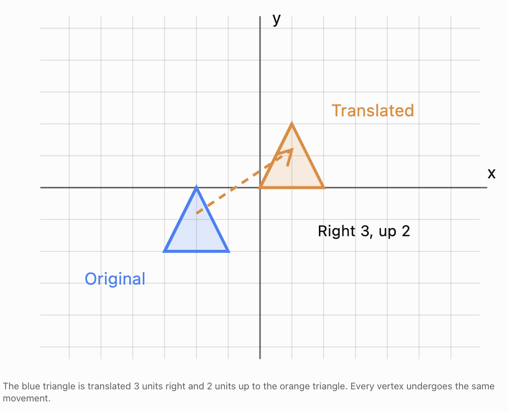
Although this illustration uses a triangle, exactly the same principle applies to graphs of functions.
Horizontal Translations
A horizontal translation moves a graph to the left or right.
Suppose the original function is:
y = f(x)
A horizontal translation is represented by:
y = f(x − h)
where h is the horizontal movement.
-
If h is positive, the graph moves right.
-
If h is negative, the graph moves left.
This can initially seem confusing because the sign inside the brackets appears opposite to the direction of movement.
Horizontal translation rules
|
Equation |
Translation |
|---|---|
|
y = f(x − 2) |
2 units right |
|
y = f(x − 5) |
5 units right |
|
y = f(x + 3) |
3 units left |
|
y = f(x + 7) |
7 units left |
Why does the sign appear reversed?
Consider:
y = x²
The original vertex occurs when x = 0.
Now consider:
y = (x − 3)²
The squared expression is zero when:
x − 3 = 0
x = 3
Therefore, the vertex moves from (0, 0) to (3, 0).
The graph moves right, even though the equation contains subtraction.
Worked Example: Translating a Parabola Right
Original function:
y = x²
Translated function:
y = (x − 2)²
The graph moves 2 units to the right.
Compare corresponding points:
|
Original point |
Translated point |
|---|---|
|
(−2, 4) |
(0, 4) |
|
(−1, 1) |
(1, 1) |
|
(0, 0) |
(2, 0) |
|
(1, 1) |
(3, 1) |
|
(2, 4) |
(4, 4) |
Notice that every x-coordinate increases by 2 while the y-coordinate remains unchanged.
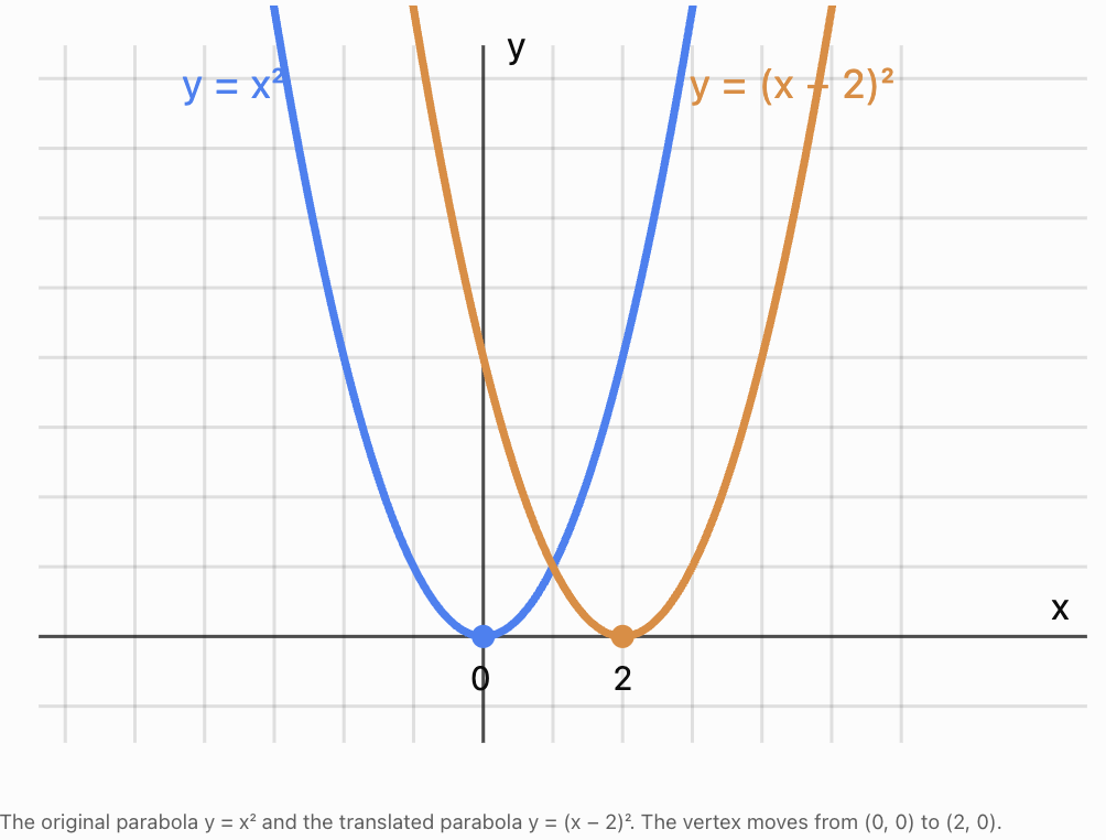
The graph's shape does not change. Only its position changes.
Worked Example: Translating a Graph Left
Original function:
y = |x|
Translated function:
y = |x + 4|
The graph moves 4 units left.
The original vertex is:
(0, 0)
The translated vertex is:
(−4, 0)
For example, the original point (2, 2) becomes:
(−2, 2)
The original point (−2, 2) becomes:
(−6, 2)
Every point moves left by 4 units.
Vertical Translations
A vertical translation moves a graph upward or downward.
For an original function:
y = f(x)
A vertical translation is represented by:
y = f(x) + k
where k is the vertical movement.
-
If k is positive, the graph moves upward.
-
If k is negative, the graph moves downward.
Vertical translation rules
|
Equation |
Translation |
|---|---|
|
y = f(x) + 3 |
3 units up |
|
y = f(x) + 8 |
8 units up |
|
y = f(x) − 2 |
2 units down |
|
y = f(x) − 6 |
6 units down |
Unlike horizontal translations, the sign of the constant outside the function directly matches the direction of movement.
Worked Example: Translating a Parabola Up
Original function:
y = x²
Translated function:
y = x² + 3
Every point moves 3 units upward.
|
Original point |
Translated point |
|---|---|
|
(−2, 4) |
(−2, 7) |
|
(−1, 1) |
(−1, 4) |
|
(0, 0) |
(0, 3) |
|
(1, 1) |
(1, 4) |
|
(2, 4) |
(2, 7) |
The x-coordinates remain unchanged.
The y-coordinates increase by 3.
The vertex moves from (0, 0) to (0, 3).
Worked Example: Translating a Graph Down
Original function:
y = √x
Translated function:
y = √x − 4
The graph moves 4 units downward.
The original starting point is:
(0, 0)
The translated starting point is:
(0, −4)
Other points translate as follows:
|
Original point |
Translated point |
|---|---|
|
(0, 0) |
(0, −4) |
|
(1, 1) |
(1, −3) |
|
(4, 2) |
(4, −2) |
|
(9, 3) |
(9, −1) |
The graph retains its original shape.
Combining Horizontal and Vertical Translations
A graph can be translated horizontally and vertically at the same time.
The general form is:
y = f(x − h) + k
where:
-
h represents the horizontal translation.
-
k represents the vertical translation.
For the point transformation:
(x, y) → (x + h, y + k)
Worked Example: Translating a parabola
Consider:
y = (x − 3)² + 2
Compare this with:
y = x²
The graph moves:
-
3 units right.
-
2 units up.
The original vertex is (0, 0).
The new vertex is (3, 2).
Other corresponding points include:
|
Original point |
Translated point |
|---|---|
|
(−2, 4) |
(1, 6) |
|
(−1, 1) |
(2, 3) |
|
(0, 0) |
(3, 2) |
|
(1, 1) |
(4, 3) |
|
(2, 4) |
(5, 6) |
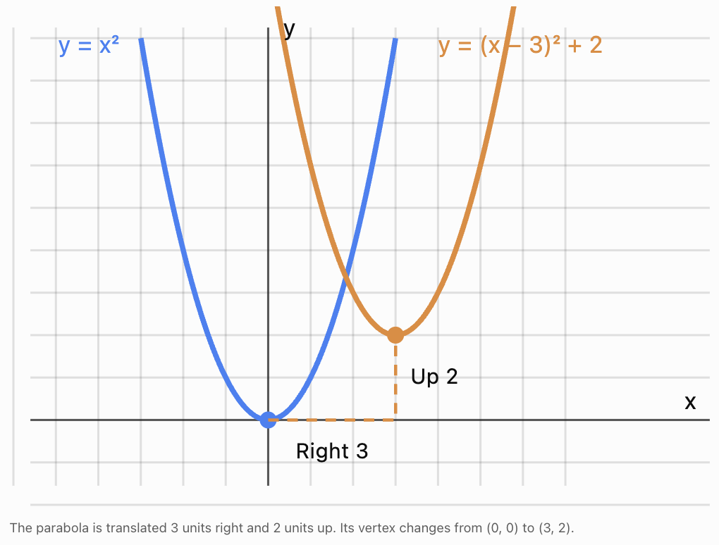
Worked Example: Left and down
Describe the transformation:
y = (x + 5)² − 4
Compared with y = x²:
-
The +5 inside the bracket means 5 units left.
-
The −4 outside the bracket means 4 units down.
The vertex is:
(−5, −4)
The shape and width of the parabola remain unchanged.
Predicting Translated Graphs
We do not always need to plot many points to predict the position of a translated graph.
Instead, we can identify important features of the original graph and move them according to the translation rule.
Important features include:
-
Vertices.
-
Turning points.
-
Endpoints.
-
Intercepts.
-
Asymptotes.
-
Points of symmetry.
-
Maximum and minimum values.
Worked Example: Translating a linear function
Original function:
y = 2x + 1
Translate the graph 3 units right and 4 units up.
Use:
g(x) = f(x − 3) + 4
Substitute:
g(x) = 2(x − 3) + 1 + 4
Expand:
g(x) = 2x − 6 + 5
g(x) = 2x − 1
The original line and translated line have the same gradient, 2.
The translated line is parallel to the original.
An important observation is that different combinations of horizontal and vertical translations can produce the same final line. For a non-horizontal straight line, the individual translations cannot always be determined uniquely from the original and final equations alone.
Worked Example: Translating an exponential function
Original function:
y = 2ˣ
Translate the graph 2 units right and 3 units down.
The translated equation is:
y = 2⁽ˣ ⁻ ²⁾ − 3
The original horizontal asymptote is:
y = 0
After translating down by 3 units, the new horizontal asymptote is:
y = −3
The original point (0, 1) becomes:
(2, −2)
The graph retains its exponential shape.
Translations of Different Function Families
The same translation rules apply to many kinds of functions.
|
Parent function |
Translated function |
Translation |
|---|---|---|
|
y = x² |
y = (x − 4)² + 1 |
Right 4, up 1 |
|
y = |x| |
y = |x + 2| − 3 |
Left 2, down 3 |
|
y = √x |
y = √(x − 5) + 2 |
Right 5, up 2 |
|
y = x³ |
y = (x + 1)³ − 4 |
Left 1, down 4 |
|
y = 2ˣ |
y = 2⁽ˣ ⁺ ³⁾ + 1 |
Left 3, up 1 |
|
y = sin x |
y = sin(x − π/2) + 2 |
Right π/2, up 2 |
The general translation rule remains:
g(x) = f(x − h) + k
The original function's shape is preserved.
Translations and the Domain and Range
Translations can change the domain and range of a function.
The domain is the set of permitted input values.
The range is the set of possible output values.
Worked Example: Square root function
Original:
y = √x
Domain:
x ≥ 0
Range:
y ≥ 0
Now translate the graph 4 units right and 2 units down:
y = √(x − 4) − 2
For the square root to be defined over the real numbers:
x − 4 ≥ 0
Therefore:
Domain: x ≥ 4
The minimum output occurs when x = 4:
y = √0 − 2 = −2
Therefore:
Range: y ≥ −2
The starting point moves from (0, 0) to (4, −2).
Worked Example: Quadratic function
Original:
y = x²
Range:
y ≥ 0
Translated:
y = (x + 3)² − 5
The vertex is (−3, −5).
Because the parabola still opens upward:
Range: y ≥ −5
The domain remains all real numbers.
General rule
If the original function has domain D and range R, a translation right by h and up by k gives:
-
New domain: every value in D increased by h.
-
New range: every value in R increased by k.
This is particularly useful when translating functions with restricted domains or ranges.
How Translations Affect Intercepts
Translations move every point of a graph, but the new x- and y-intercepts do not always come directly from translating the original intercepts.
An intercept is defined by its position on an axis.
After translation, a point that was originally on an axis may no longer be on that axis.
Worked Example
Original:
y = x²
Translated:
y = (x − 2)² − 4
The vertex is (2, −4).
To find the x-intercepts, set y = 0:
0 = (x − 2)² − 4
(x − 2)² = 4
x − 2 = ±2
Therefore:
x = 0 or x = 4
The x-intercepts are:
(0, 0) and (4, 0)
To find the y-intercept, set x = 0:
y = (0 − 2)² − 4
y = 0
The y-intercept is:
(0, 0)
This example shows that intercepts should be recalculated from the translated equation when needed.
Sketching Translated Graphs
A systematic method makes sketching translations much easier.
Step 1: Identify the parent function
For example:
y = x²
Recognise the familiar U-shaped parabola.
Step 2: Identify the translations
For:
y = (x − 2)² + 3
The graph moves 2 units right and 3 units up.
Step 3: Move the key points
The vertex moves:
(0, 0) → (2, 3)
Other points:
(−1, 1) → (1, 4)
(1, 1) → (3, 4)
(−2, 4) → (0, 7)
(2, 4) → (4, 7)
Step 4: Plot the points
Mark the new vertex and several corresponding points.
Step 5: Draw the graph
Connect the points using the same shape as the original function.
Step 6: Label important features
Include the equation, vertex, axes, and any important intercepts or asymptotes.
Describing a Translation from Two Equations
Sometimes we are given an original function and a transformed function and must describe the movement.
Worked Example
Original:
y = x²
Transformed:
y = (x + 6)² + 4
The graph moves:
6 units left and 4 units up.
Worked Example
Original:
y = |x|
Transformed:
y = |x − 3| − 7
The graph moves:
3 units right and 7 units down.
Worked Example
Original:
y = √x
Transformed:
y = √(x + 2) + 5
The graph moves:
2 units left and 5 units up.
Finding the Equation from a Translation
We can also work backwards.
Worked Example: From a description
The graph of y = x² is translated 5 units right and 2 units down.
Start with:
y = f(x)
Apply:
g(x) = f(x − 5) − 2
Therefore:
y = (x − 5)² − 2
Worked Example: From a new vertex
A parabola has the same shape and orientation as y = x², but its vertex is (−3, 4).
The equation is:
y = (x + 3)² + 4
Worked Example: Translating an absolute value graph
The graph of y = |x| is translated 4 units left and 1 unit down.
The equation is:
y = |x + 4| − 1
The vertex is (−4, −1).
Applications of Translations
Graph translations are useful because they allow mathematical models to be adjusted without rebuilding them from the beginning.
Physics: Vertical motion
Suppose the height of an object is modeled by:
h(t) = −5t² + 20t
where h is height in metres and t is time in seconds.
If the object is launched from a platform 15 m above the original reference level, its height becomes:
H(t) = −5t² + 20t + 15
The new graph is translated 15 units upward relative to the original height-time graph.
The parabolic shape remains unchanged.
This model assumes the same initial vertical velocity and gravitational acceleration, with air resistance neglected.
Business: Fixed operating costs
Suppose the variable production cost for n products is:
C = 8n
If a business also has a fixed cost of $200, the new cost function is:
C = 8n + 200
The graph moves upward by 200 units.
The gradient remains 8, meaning the cost still increases by $8 per additional product.
Biology: Shifting a growth model
Suppose an idealised growth model is:
P(t) = 100(1.1)ᵗ
If the same growth pattern begins 3 years later, its equation can be written:
P(t) = 100(1.1)⁽ᵗ ⁻ ³⁾
This represents a horizontal translation 3 years to the right.
The model has been shifted in time without changing its exponential growth pattern.
Comparing Translations with Other Transformations
Not every change to an equation represents a translation.
Consider the parent function:
y = x²
|
Equation |
Transformation |
|---|---|
|
y = x² + 4 |
Translation 4 units up |
|
y = (x − 4)² |
Translation 4 units right |
|
y = 2x² |
Vertical stretch by factor 2 |
|
y = −x² |
Reflection in the x-axis |
|
y = (2x)² |
Horizontal compression by factor 1/2 |
|
y = (x − 3)² + 2 |
Right 3 and up 2 |
A translation changes position without changing shape or orientation.
A stretch or compression changes the dimensions of the graph.
A reflection changes its orientation.
These distinctions become especially important when studying combined function transformations.
Common Mistakes
Confusing horizontal directions
For horizontal translations, the sign inside the function appears opposite to the movement.
y = f(x − 3) moves right 3 units.
y = f(x + 3) moves left 3 units.
Confusing vertical directions
Vertical translations follow the sign outside the function.
y = f(x) + 4 moves up 4 units.
y = f(x) − 4 moves down 4 units.
Changing the shape of the graph
Translations do not stretch, compress, or reflect a graph.
Moving only the vertex
Every point on the graph must move by the same amount.
Incorrectly translating coordinates
A translation right 4 and down 2 changes (x, y) to (x + 4, y − 2), not (x − 4, y + 2).
Forgetting brackets
The equations y = (x − 3)² and y = x² − 3 represent different translations.
Assuming intercepts simply remain intercepts
A translated point that was originally an intercept may no longer lie on an axis. Recalculate intercepts when necessary.
Ignoring domain and range changes
Horizontal translations may change the domain, while vertical translations may change the range.
Key Terms
-
Transformation: A change to the position, size, or orientation of a graph or shape.
-
Translation: A transformation that moves every point the same distance in the same direction.
-
Horizontal translation: A movement left or right.
-
Vertical translation: A movement up or down.
-
Parent function: A basic function used as a reference for transformations.
-
Translated function: A function obtained by shifting a parent function.
-
Coordinate rule: A rule describing how point coordinates change under a transformation.
-
Vertex: The turning point of a parabola or the corner of an absolute value graph.
-
Domain: The set of allowed input values.
-
Range: The set of possible output values.
-
Intercept: A point where a graph crosses or touches a coordinate axis.
-
Asymptote: A line that a graph approaches in a specified limiting direction.
-
Function notation: A way of expressing a function using symbols such as f(x).
-
Invariant shape: A shape that remains unchanged under a transformation.
-
Graph sketching: Representing the main features of a function on coordinate axes.
Key Takeaways
-
A translation moves every point of a graph by the same amount.
-
Translations preserve shape, size, and orientation.
-
Horizontal translations are represented by y = f(x − h).
-
Vertical translations are represented by y = f(x) + k.
-
The combined translation rule is y = f(x − h) + k.
-
Positive h moves a graph right; negative h moves it left.
-
Positive k moves a graph up; negative k moves it down.
-
A point (x, y) becomes (x + h, y + k).
-
Key points such as vertices, endpoints, and asymptotes help us sketch translated graphs.
-
The domain and range may change after a translation.
-
Intercepts should be recalculated when necessary.
-
Translation rules apply to quadratic, linear, absolute value, square root, exponential, trigonometric, and other functions.
Check Your Understanding
Recall and Understanding
1. Define a translation and explain which properties of a graph remain unchanged.
2. Describe the difference between horizontal and vertical translations.
3. Explain why y = (x − 4)² represents a translation to the right rather than to the left.
4. State the general equation for translating y = f(x) by h units horizontally and k units vertically.
Application
5. Describe the translation from y = x² to y = (x − 5)².
6. Describe the translation from y = |x| to y = |x + 3| − 4.
7. The point (2, 7) is translated 4 units left and 6 units down. Find its new coordinates.
8. Write the equation of y = x² after translating it 3 units right and 5 units up.
9. The graph of y = √x is translated 2 units left and 3 units down. Write its new equation and state its domain and range.
10. The graph of y = 2ˣ is translated 4 units right and 2 units up. Write the transformed equation and state its horizontal asymptote.
Analysis and Challenge
11. A parabola has the same shape and orientation as y = x², but its vertex is (−4, 6). Write its equation.
12. The graph of y = (x − 2)² + 3 is translated 5 units left and 4 units down. Find the resulting equation and vertex.
13. A function passes through the points (−2, 3), (0, 1), and (4, 5). Find the coordinates of these points after translating the graph 3 units right and 2 units down.
14. A quadratic function is given by y = (x − 3)² − 9. Determine its vertex, x-intercepts, and y-intercept.
15. A student claims that y = (x + 5)² − 2 is obtained from y = x² by moving 5 units right and 2 units down. Explain the error and give the correct translation.
Answers to Check Your Understanding
1. A translation moves every point of a graph by the same amount and in the same direction. Its shape, size, and orientation remain unchanged.
2. A horizontal translation moves a graph left or right and changes the input of the function. A vertical translation moves a graph up or down and changes the output.
3. The expression x − 4 equals zero when x = 4, so the vertex moves from x = 0 to x = 4. Therefore, the graph moves 4 units right.
4. The general equation is:
y = f(x − h) + k
5. The graph moves 5 units right.
6. The graph moves 3 units left and 4 units down.
7.
(2, 7) → (2 − 4, 7 − 6)
(−2, 1)
8.
y = (x − 3)² + 5
9.
New equation:
y = √(x + 2) − 3
Domain:
x ≥ −2
Range:
y ≥ −3
10.
New equation:
y = 2⁽ˣ ⁻ ⁴⁾ + 2
Horizontal asymptote:
y = 2
11.
Vertex = (−4, 6)
y = (x + 4)² + 6
12.
Original vertex:
(2, 3)
Translate left 5:
x = 2 − 5 = −3
Translate down 4:
y = 3 − 4 = −1
New vertex:
(−3, −1)
New equation:
y = (x + 3)² − 1
13.
Apply:
(x, y) → (x + 3, y − 2)
(−2, 3) → (1, 1)
(0, 1) → (3, −1)
(4, 5) → (7, 3)
14.
Given:
y = (x − 3)² − 9
Vertex:
(3, −9)
For x-intercepts, set y = 0:
(x − 3)² − 9 = 0
(x − 3)² = 9
x − 3 = ±3
x = 0 or x = 6
x-intercepts:
(0, 0) and (6, 0)
For the y-intercept, set x = 0:
y = (0 − 3)² − 9 = 0
y-intercept:
(0, 0)
15.
The student has confused the direction of the horizontal translation.
The expression x + 5 means the graph moves 5 units left, not right.
The −2 outside the squared expression means the graph moves 2 units down.
Correct translation: 5 units left and 2 units down.
The new vertex is (−5, −2).
Final Summary
Translations allow us to move graphs horizontally and vertically while preserving their shape and orientation.
By understanding how changes inside and outside a function affect its graph, we can predict transformations, sketch graphs accurately, and connect algebraic equations with geometric movements.
The most important relationship is:
y = f(x − h) + k
This represents a translation of h units horizontally and k units vertically.
Mastering translations provides an essential foundation for studying more advanced function transformations, graph analysis, and mathematical modeling.
2. Reflections
Learning outcomes
- I can reflect graphs across the x-axis.
- I can reflect graphs across the y-axis.
- I can predict reflected equations.
- I can compare original and reflected graphs.
- I can identify reflections from graphs.
Introduction
A reflection is a transformation that produces a mirror image of a graph across a line.
In coordinate geometry, two of the most important reflections are:
-
Reflection across the x-axis.
-
Reflection across the y-axis.
Reflections change the orientation of a graph while preserving its shape and size.
For example, consider the quadratic function:
y = x²
Its graph is a parabola opening upward.
If we reflect it across the x-axis, the equation becomes:
y = −x²
The new parabola opens downward.
Now consider:
y = (x − 2)²
Reflecting this graph across the y-axis gives:
y = (x + 2)²
The vertex moves from (2, 0) to (−2, 0).
Reflections are important because they help us understand how negative signs affect functions, how graphs behave under transformations, and how algebraic equations are connected to geometric symmetry.
In this topic, we will explore how to reflect graphs, predict reflected equations, compare original and transformed functions, and recognise reflections from graphs.
What Is a Reflection?
A reflection is a transformation in which every point on a graph is moved to the opposite side of a fixed line, called the line of reflection.
Each point and its reflected image are the same perpendicular distance from the line of reflection.
For example, if a point lies 3 units above the x-axis, its reflection across the x-axis lies 3 units below it.
During a reflection:
-
The shape remains unchanged.
-
The size remains unchanged.
-
Distances between points remain unchanged.
-
The graph's orientation is reversed.
-
Points on the line of reflection remain fixed.
A reflection is therefore a rigid transformation, also called an isometry.
Visualising Reflections
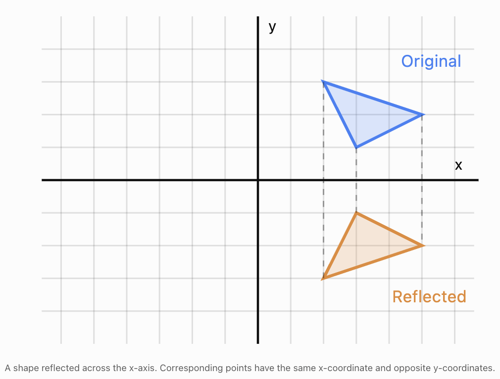
The same principle applies to graphs of mathematical functions.
Reflections Across the x-Axis
A reflection across the x-axis changes the sign of every y-coordinate.
The coordinate rule is:
(x, y) → (x, −y)
For example:
-
(2, 3) becomes (2, −3).
-
(−4, 5) becomes (−4, −5).
-
(3, −2) becomes (3, 2).
-
(0, 0) remains (0, 0).
The x-coordinate does not change.
Equation rule
If the original function is:
y = f(x)
its reflection across the x-axis is:
y = −f(x)
The negative sign is placed outside the entire function.
This means every output is multiplied by −1.
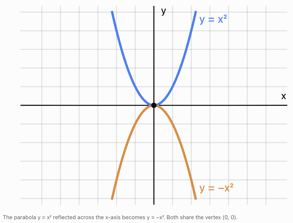
Worked Example: Reflecting a parabola
Original:
y = x²
Reflection across the x-axis:
y = −x²
The original graph opens upward.
The reflected graph opens downward.
|
x |
Original y = x² |
Reflected y = −x² |
|---|---|---|
|
−2 |
4 |
−4 |
|
−1 |
1 |
−1 |
|
0 |
0 |
0 |
|
1 |
1 |
−1 |
|
2 |
4 |
−4 |
Every y-value changes sign.
Reflecting More Complicated Functions Across the x-Axis
The reflection rule applies to the entire function, not just one term.
Worked Example: Linear function
Original:
y = 2x + 3
Reflection across the x-axis:
y = −(2x + 3)
Distribute the negative sign:
y = −2x − 3
The original line has gradient 2 and y-intercept 3.
The reflected line has gradient −2 and y-intercept −3.
Worked Example: Quadratic function
Original:
y = x² − 4x + 1
Reflection across the x-axis:
y = −(x² − 4x + 1)
Expand:
y = −x² + 4x − 1
Every term changes sign.
Worked Example: Absolute value function
Original:
y = |x − 3| + 2
Reflection across the x-axis:
y = −(|x − 3| + 2)
Simplify:
y = −|x − 3| − 2
The original graph has a minimum at (3, 2).
The reflected graph has a maximum at (3, −2).
Reflections Across the y-Axis
A reflection across the y-axis changes the sign of every x-coordinate.
The coordinate rule is:
(x, y) → (−x, y)
For example:
-
(3, 4) becomes (−3, 4).
-
(−2, 5) becomes (2, 5).
-
(4, −3) becomes (−4, −3).
-
(0, 2) remains (0, 2).
The y-coordinate does not change.
Equation rule
If the original function is:
y = f(x)
its reflection across the y-axis is:
y = f(−x)
We replace every occurrence of x with −x.
Worked Example: Reflecting a linear function
Original:
y = 3x + 2
Replace x with −x:
y = 3(−x) + 2
Simplify:
y = −3x + 2
The original line has gradient 3.
The reflected line has gradient −3.
The y-intercept remains 2 because points on the y-axis are unchanged.
Worked Example: Reflecting a parabola
Original:
y = (x − 4)²
Reflect across the y-axis:
y = (−x − 4)²
Factor out −1 inside the bracket:
y = [−(x + 4)]²
Since squaring removes the negative sign:
y = (x + 4)²
The original vertex is (4, 0).
The reflected vertex is (−4, 0).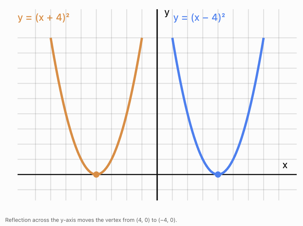
Reflecting Polynomial Functions Across the y-Axis
When reflecting a polynomial across the y-axis, replace every x with −x and simplify.
Worked Example
Original:
y = x³ + 2x² − 5x + 4
Replace x with −x:
y = (−x)³ + 2(−x)² − 5(−x) + 4
Simplify each term:
(−x)³ = −x³
(−x)² = x²
−5(−x) = 5x
Therefore:
y = −x³ + 2x² + 5x + 4
Notice:
-
Odd powers of x change sign.
-
Even powers of x do not change sign.
-
Constant terms remain unchanged.
This pattern can make reflections of polynomial functions much faster.
Comparing Reflections Across the x-Axis and y-Axis
Although both transformations create mirror images, they affect coordinates and equations differently.
|
Feature |
Reflection across x-axis |
Reflection across y-axis |
|---|---|---|
|
Coordinate rule |
(x, y) → (x, −y) |
(x, y) → (−x, y) |
|
Function rule |
y = −f(x) |
y = f(−x) |
|
Coordinate that changes sign |
y |
x |
|
Axis containing fixed points |
x-axis |
y-axis |
|
Effect on outputs |
Negates outputs |
Reverses inputs |
|
Example from y = 2x + 3 |
y = −2x − 3 |
y = −2x + 3 |
The distinction is especially important when reflecting functions that are not symmetric.
Even and Odd Functions
Some graphs have natural symmetry.
This can cause a reflection to produce exactly the same graph.
Even functions
A function is even if:
f(−x) = f(x)
Its graph is symmetric about the y-axis.
Examples include:
-
f(x) = x²
-
f(x) = x⁴
-
f(x) = |x|
-
f(x) = cos x
For example:
f(x) = x²
f(−x) = (−x)² = x²
Therefore, reflecting y = x² across the y-axis produces the same graph.
Odd functions
A function is odd if:
f(−x) = −f(x)
Its graph is symmetric about the origin.
Examples include:
-
f(x) = x
-
f(x) = x³
-
f(x) = sin x
For example:
f(x) = x³
f(−x) = (−x)³ = −x³
Therefore:
f(−x) = −f(x)
A reflection of an odd function across the y-axis produces the same graph as reflecting it across the x-axis.
Reflecting Absolute Value Functions
Absolute value graphs are particularly useful for understanding reflections because they have a distinctive V-shape.
Worked Example: Across the x-axis
Original:
y = |x|
Reflected:
y = −|x|
The original graph opens upward.
The reflected graph opens downward.
The vertex remains at (0, 0).
Worked Example: Across the y-axis
Original:
y = |x − 3|
Reflected:
y = |−x − 3|
Simplify:
y = |x + 3|
The vertex moves from (3, 0) to (−3, 0).
Worked Example: A translated absolute value function
Original:
y = |x − 2| + 4
Reflect across the x-axis:
y = −(|x − 2| + 4)
y = −|x − 2| − 4
Reflect the original across the y-axis instead:
y = |−x − 2| + 4
y = |x + 2| + 4
These transformations produce different graphs.
Reflecting Square Root Functions
Square root functions have restricted domains, making them useful for understanding how reflections affect domain and range.
Worked Example: Across the x-axis
Original:
y = √x
Domain:
x ≥ 0
Range:
y ≥ 0
Reflect across the x-axis:
y = −√x
Domain:
x ≥ 0
Range:
y ≤ 0
The graph is now below or on the x-axis.
Worked Example: Across the y-axis
Original:
y = √x
Reflect across the y-axis:
y = √(−x)
For the square root to be defined:
−x ≥ 0
Therefore:
x ≤ 0
Domain:
x ≤ 0
Range:
y ≥ 0
The graph now extends to the left of the y-axis.
Worked Example: Reflecting a translated square root function
Original:
y = √(x − 4) + 2
Its starting point is (4, 2).
Reflect across the y-axis:
y = √(−x − 4) + 2
The starting point becomes:
(−4, 2)
The reflected domain is:
x ≤ −4
The range remains:
y ≥ 2
Reflecting Exponential Functions
Exponential graphs can also be reflected.
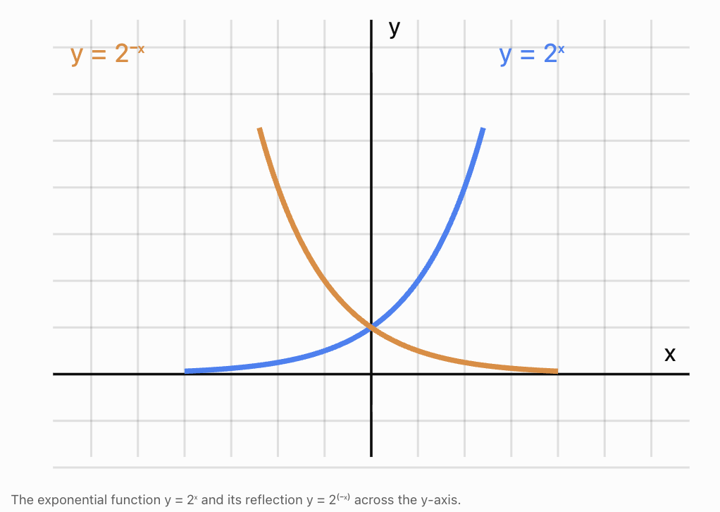
Consider:
y = 2ˣ
Reflection across the x-axis
y = −2ˣ
This means y = −(2ˣ).
The graph lies below the x-axis.
Its horizontal asymptote remains y = 0.
Reflection across the y-axis
y = 2⁽⁻ˣ⁾
This can also be written as:
y = (1/2)ˣ
The original function increases as x increases.
The reflected function decreases as x increases.
Reflecting Graphs with Translations
Reflections can be combined with horizontal and vertical translations.
Consider:
y = −(x − 3)² + 4
Starting with:
y = x²
We can describe the transformations as:
-
Translate 3 units right.
-
Reflect across the x-axis.
-
Translate 4 units up.
The final vertex is:
(3, 4)
The parabola opens downward.
The transformations must be interpreted carefully because changing their order can sometimes change the final result.
Worked Example: Combining transformations
Start with:
y = |x|
Reflect across the x-axis:
y = −|x|
Translate 2 units left:
y = −|x + 2|
Translate 3 units down:
y = −|x + 2| − 3
The final vertex is (−2, −3).
The graph opens downward.
Identifying Reflections from Graphs
Sometimes we are given two graphs rather than equations.
To determine whether one is a reflection of the other, compare corresponding points and key features.
Reflection across the x-axis
Look for:
-
Matching x-coordinates.
-
Opposite y-coordinates.
-
Equal distances above and below the x-axis.
-
Reversed vertical orientation.
For example:
Original vertex: (2, 5)
Reflected vertex: (2, −5)
This is consistent with reflection across the x-axis.
Reflection across the y-axis
Look for:
-
Opposite x-coordinates.
-
Matching y-coordinates.
-
Equal distances left and right of the y-axis.
-
Reversed horizontal orientation.
For example:
Original vertex: (4, −2)
Reflected vertex: (−4, −2)
This is consistent with reflection across the y-axis.
Important limitation
A single matching pair of points does not prove that an entire graph has been reflected.
To confirm a reflection, the same coordinate rule must apply to every corresponding point.
Reflecting Graphs Step by Step
A reliable sketching method is:
Identify the original function.
Recognise its basic shape and important features.
Choose the line of reflection.
Determine whether the reflection is across the x-axis or y-axis.
Apply the coordinate rule.
Across the x-axis:
(x, y) → (x, −y)
Across the y-axis:
(x, y) → (−x, y)
Reflect important points.
These may include vertices, endpoints, intercepts, and turning points.
Sketch the reflected graph.
Preserve the original shape and size.
Check symmetry.
Corresponding points should be equally distant from the reflection axis.
Reflections and the Domain and Range
Reflections can affect the domain and range of functions.
Reflection across the x-axis
The x-values remain unchanged, so the domain remains the same.
The y-values change sign, so the range is reflected across zero.
Example:
Original:
y = x² + 2
Domain: all real numbers
Range: y ≥ 2
Reflected:
y = −x² − 2
Domain: all real numbers
Range: y ≤ −2
Reflection across the y-axis
The y-values remain unchanged, so the range remains the same.
The x-values change sign, so the domain is reflected across zero.
Example:
Original:
y = √(x − 3)
Domain: x ≥ 3
Range: y ≥ 0
Reflected:
y = √(−x − 3)
Domain: x ≤ −3
Range: y ≥ 0
These rules are particularly important for functions with restricted domains and ranges.
Reflecting Across Both Axes
A graph can be reflected across the x-axis and then across the y-axis.
Starting with:
y = f(x)
Reflect across the x-axis:
y = −f(x)
Then reflect across the y-axis:
y = −f(−x)
The coordinate rule is:
(x, y) → (−x, −y)
This is equivalent to a rotation of 180° about the origin.
Worked Example
Original:
y = x³ + 2
Reflect across both axes:
y = −f(−x)
Substitute:
y = −[(−x)³ + 2]
Simplify:
y = −[−x³ + 2]
y = x³ − 2
The final graph is equivalent to translating the original cubic graph downward by 4 units, although the transformation used here is a pair of reflections.
Applications of Reflections
Physics: Opposite directions
Suppose the vertical position of an object relative to a reference level is represented by:
y = f(t)
If we reverse the sign convention for vertical position, the new coordinate becomes:
y = −f(t)
The graph is reflected across the horizontal axis.
This is useful when comparing upward-positive and downward-positive coordinate systems.
Economics: Profit and loss
Suppose a function P(x) represents profit.
The function:
L(x) = −P(x)
represents the negative of profit, which may be interpreted as a loss balance under a suitable sign convention.
The graph of L(x) is the reflection of P(x) across the x-axis.
Signal processing
Signals can be reflected in two important ways.
Amplitude inversion:
g(t) = −f(t)
This reflects the signal across the horizontal axis.
Time reversal:
g(t) = f(−t)
This reflects the signal across the vertical axis.
These transformations are important in mathematics, physics, electronics, and signal analysis.
Common Mistakes
Confusing reflections across the two axes
Across the x-axis, change the sign of the output.
Across the y-axis, change the sign of the input.
Negating only one term
For an x-axis reflection:
y = −(x² + 3x + 2)
Correct:
y = −x² − 3x − 2
Not:
y = −x² + 3x + 2
Forgetting to replace every x
For a y-axis reflection, every occurrence of x must be replaced by −x.
Assuming all reflections change the graph
Some functions are symmetric about an axis, so reflecting them across that axis produces the same graph.
Confusing reflections with translations
Translations move graphs without reversing their orientation. Reflections produce mirror images.
Incorrectly simplifying powers
(−x)² = x²
(−x)³ = −x³
Ignoring domain and range changes
Reflections may change domain or range restrictions.
Assuming the reflection of every function is different
Even functions are unchanged by y-axis reflection.
Key Terms
-
Reflection: A transformation that produces a mirror image across a line.
-
Line of reflection: The fixed line across which a graph is reflected.
-
x-axis reflection: A transformation changing (x, y) to (x, −y).
-
y-axis reflection: A transformation changing (x, y) to (−x, y).
-
Transformation: A change to the position, size, or orientation of a graph.
-
Rigid transformation: A transformation preserving distances and shape.
-
Coordinate rule: A rule describing how points move under a transformation.
-
Function notation: A way of representing functions using symbols such as f(x).
-
Even function: A function satisfying f(−x) = f(x).
-
Odd function: A function satisfying f(−x) = −f(x).
-
Symmetry: A property in which a graph matches itself under a specified transformation.
-
Vertex: A turning point of a parabola or the corner of an absolute value graph.
-
Domain: The set of permitted input values.
-
Range: The set of possible output values.
-
Intercept: A point where a graph meets a coordinate axis.
-
Asymptote: A line that a graph approaches in a specified limiting direction.
-
Amplitude inversion: A transformation changing f(x) to −f(x).
-
Time reversal: A transformation changing f(t) to f(−t).
Key Takeaways
-
Reflections produce mirror images of graphs.
-
Reflecting across the x-axis changes (x, y) to (x, −y).
-
Reflecting across the y-axis changes (x, y) to (−x, y).
-
The equation for an x-axis reflection is y = −f(x).
-
The equation for a y-axis reflection is y = f(−x).
-
Reflections preserve the shape and size of a graph.
-
Reflecting across the x-axis changes the sign of every output.
-
Reflecting across the y-axis reverses the sign of every input.
-
Even functions are symmetric about the y-axis.
-
Odd functions are symmetric about the origin.
-
Reflections can be combined with translations and other transformations.
-
Domain and range restrictions must be considered when reflecting graphs.
-
Reflected graphs can be identified by comparing corresponding points and their distances from the reflection axis.
Check Your Understanding
Recall and Understanding
1. Define a reflection and explain which properties of a graph remain unchanged.
2. State the coordinate rule for reflection across the x-axis.
3. State the coordinate rule for reflection across the y-axis.
4. Explain the difference between y = −f(x) and y = f(−x).
Application
5. Reflect the point (4, −7) across the x-axis.
6. Reflect the point (−3, 5) across the y-axis.
7. Write the equation obtained by reflecting y = 3x + 4 across the x-axis.
8. Write the equation obtained by reflecting y = x² − 6x + 2 across the y-axis.
9. Reflect y = |x − 5| + 3 across the x-axis. State the vertex of the reflected graph.
10. Reflect y = √(x − 4) across the y-axis. State the domain of the reflected function.
Analysis and Challenge
11. A parabola has equation y = (x − 3)² − 4. Reflect it across the y-axis and state its new vertex.
12. A function is defined by f(x) = x³ − 2x. Determine whether it is even, odd, or neither.
13. Reflect y = 2ˣ across both the x-axis and y-axis. Write the resulting equation.
14. A graph passes through (−2, 3), (0, −1), and (4, 5). Find the coordinates of the reflected points after reflection across the x-axis.
15. A student claims that reflecting y = x² + 4 across the y-axis produces y = −x² + 4. Explain the error and give the correct equation.
Answers to Check Your Understanding
1. A reflection produces a mirror image across a line. Shape, size, and distances between points remain unchanged.
2.
(x, y) → (x, −y)
3.
(x, y) → (−x, y)
4.
y = −f(x) reflects a graph across the x-axis by negating the outputs.
y = f(−x) reflects a graph across the y-axis by reversing the inputs.
5.
(4, −7) → (4, 7)
6.
(−3, 5) → (3, 5)
7.
Original:
y = 3x + 4
Reflected:
y = −(3x + 4)
y = −3x − 4
8.
Original:
y = x² − 6x + 2
Replace x with −x:
y = (−x)² − 6(−x) + 2
y = x² + 6x + 2
9.
Original:
y = |x − 5| + 3
Reflect across the x-axis:
y = −(|x − 5| + 3)
y = −|x − 5| − 3
Vertex:
(5, −3)
10.
Original:
y = √(x − 4)
Reflect across the y-axis:
y = √(−x − 4)
For the square root to be defined:
−x − 4 ≥ 0
Domain: x ≤ −4
11.
Original:
y = (x − 3)² − 4
Reflect across the y-axis:
y = (−x − 3)² − 4
Simplify:
y = (x + 3)² − 4
New vertex:
(−3, −4)
12.
f(x) = x³ − 2x
Calculate:
f(−x) = (−x)³ − 2(−x)
= −x³ + 2x
= −(x³ − 2x)
Therefore:
f(−x) = −f(x)
The function is odd.
13.
Original:
y = 2ˣ
Reflect across the x-axis:
y = −2ˣ
Reflect across the y-axis:
y = −2⁽⁻ˣ⁾
Equivalent form:
y = −(1/2)ˣ
14.
Reflect across the x-axis using:
(x, y) → (x, −y)
(−2, 3) → (−2, −3)
(0, −1) → (0, 1)
(4, 5) → (4, −5)
15.
The student has confused reflection across the y-axis with reflection across the x-axis.
For a y-axis reflection, replace x with −x:
y = (−x)² + 4
Since (−x)² = x²:
y = x² + 4
The original graph is symmetric about the y-axis, so the reflection produces the same graph.
Final Summary
Reflections are fundamental graph transformations that produce mirror images across coordinate axes.
Understanding how reflections affect coordinates and function equations allows us to predict, sketch, and compare transformed graphs accurately.
The two most important rules are:
Across the x-axis: y = −f(x)
Across the y-axis: y = f(−x)
These principles provide an important foundation for understanding symmetry, function transformations, and more advanced mathematical relationships.
3. Stretches and Compressions
Learning outcomes
- I can describe vertical stretches.
- I can describe vertical compressions.
- I can compare transformed graphs.
- I can identify transformations from equations.
- I can sketch transformed graphs.
Introduction
Not all graph transformations involve moving a graph to a different position or reflecting it across an axis. Some transformations change the graph's shape by stretching or compressing it.
A stretch makes a graph larger in a particular direction, while a compression makes it smaller in that direction.
For example, consider the quadratic function:
y = x²
Its graph is a parabola with a vertex at (0, 0).
Now consider:
y = 3x²
For every value of x, the output is three times the original output. This is called a vertical stretch by a factor of 3.
Alternatively:
y = 0.5x²
Every output is half its original value. This is a vertical compression by a factor of 0.5.
These transformations are important because they allow us to change the shape of a graph while preserving its general mathematical structure.
Stretches and compressions appear in quadratic functions, absolute value functions, exponential functions, trigonometric functions, and many mathematical models used in science and engineering.
What Are Stretches and Compressions?
A stretch or compression is a transformation that changes the distance of points from a particular axis.
There are two main types:
-
Vertical stretches and compressions: Change the y-coordinates of points.
-
Horizontal stretches and compressions: Change the x-coordinates of points.
In this topic, our main focus is on vertical transformations, although horizontal transformations will also be introduced for comparison.
Unlike translations and reflections, stretches and compressions generally change the shape or dimensions of a graph.
However, some points may remain unchanged, especially points lying on the relevant axis.
Vertical Stretches
A vertical stretch moves points farther from the x-axis.
For an original function:
y = f(x)
A vertical stretch by a factor of a is represented by:
y = af(x)
where:
a > 1
Every y-coordinate is multiplied by a.
The x-coordinates remain unchanged.
Coordinate rule
(x, y) → (x, ay)
For example, a vertical stretch by a factor of 3 transforms:
-
(1, 2) → (1, 6)
-
(2, 4) → (2, 12)
-
(−1, −3) → (−1, −9)
-
(0, 0) → (0, 0)
Points above the x-axis move farther upward.
Points below the x-axis move farther downward.
Points on the x-axis remain fixed.
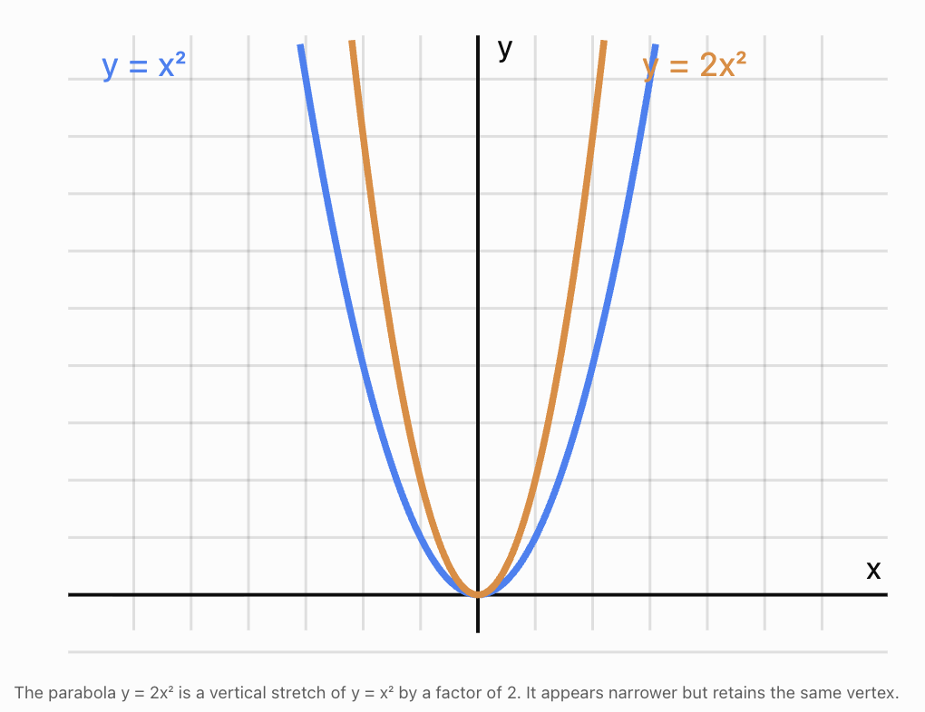
Worked Example: Vertical Stretch of a Quadratic Function
Original function:
y = x²
Transformed function:
y = 2x²
The transformed function is a vertical stretch by a factor of 2.
Compare the values:
|
x |
Original y = x² |
Stretched y = 2x² |
|---|---|---|
|
−2 |
4 |
8 |
|
−1 |
1 |
2 |
|
0 |
0 |
0 |
|
1 |
1 |
2 |
|
2 |
4 |
8 |
Every output is doubled.
The vertex remains at (0, 0).
The transformed parabola appears narrower than the original because its height increases more quickly as we move away from the vertex.
Vertical Compressions
A vertical compression moves points closer to the x-axis.
For an original function:
y = f(x)
a vertical compression is represented by:
y = af(x)
where:
0 < a < 1
Every y-coordinate is multiplied by a number between 0 and 1.
Coordinate rule
(x, y) → (x, ay)
For example, a vertical compression by a factor of 0.5 transforms:
-
(1, 6) → (1, 3)
-
(2, 8) → (2, 4)
-
(−1, −4) → (−1, −2)
-
(0, 0) → (0, 0)
Points move closer to the x-axis.
Worked Example: Vertical Compression of a Quadratic Function
Original:
y = x²
Transformed:
y = 0.5x²
The transformed function is a vertical compression by a factor of 0.5.
|
x |
Original y = x² |
Compressed y = 0.5x² |
|---|---|---|
|
−2 |
4 |
2 |
|
−1 |
1 |
0.5 |
|
0 |
0 |
0 |
|
1 |
1 |
0.5 |
|
2 |
4 |
2 |
The outputs are halved.
The parabola appears wider because it increases more slowly as x moves away from zero.
Comparing Vertical Stretches and Compressions
The coefficient outside a function determines the vertical scaling.
|
Equation |
Transformation |
|---|---|
|
y = f(x) |
Original graph |
|
y = 2f(x) |
Vertical stretch by factor 2 |
|
y = 4f(x) |
Vertical stretch by factor 4 |
|
y = 0.5f(x) |
Vertical compression by factor 0.5 |
|
y = 0.25f(x) |
Vertical compression by factor 0.25 |
|
y = −2f(x) |
Vertical stretch by factor 2 and reflection across x-axis |
|
y = −0.5f(x) |
Vertical compression by factor 0.5 and reflection across x-axis |
The absolute value of the coefficient determines the scale.
The sign determines whether an additional reflection occurs.
General rule
For:
y = af(x)
-
|a| > 1: vertical stretch.
-
0 < |a| < 1: vertical compression.
-
a < 0: reflection across the x-axis as well.
-
a = 1: no vertical scaling.
-
a = −1: reflection across the x-axis only.
-
a = 0: all outputs become zero, collapsing the graph onto the x-axis over its domain.
Stretches and Compressions of Absolute Value Functions
Absolute value functions provide a clear visual example of vertical scaling.
The parent function is:
y = |x|
Its graph has a V-shape with a vertex at (0, 0).
Worked Example: Vertical stretch
Consider:
y = 3|x|
Every output is multiplied by 3.
|
x |
y = |x| |
y = 3|x| |
|---|---|---|
|
−2 |
2 |
6 |
|
−1 |
1 |
3 |
|
0 |
0 |
0 |
|
1 |
1 |
3 |
|
2 |
2 |
6 |
The graph becomes steeper, and its V-shape appears narrower.
Worked Example: Vertical compression
Consider:
y = 0.25|x|
Every output is multiplied by 0.25.
The graph becomes less steep and appears wider.
For example, the original point (4, 4) becomes (4, 1).
The vertex remains at (0, 0).
Worked Example: Scaling and reflection
Consider:
y = −2|x|
The coefficient −2 produces two transformations:
-
A vertical stretch by a factor of 2.
-
A reflection across the x-axis.
The graph opens downward and is steeper than y = |x|.
Stretches and Compressions of Linear Functions
Vertical scaling also applies to straight lines.
Consider:
f(x) = 2x + 1
Apply a vertical stretch by a factor of 3:
g(x) = 3f(x)
g(x) = 3(2x + 1)
g(x) = 6x + 3
The original gradient is 2.
The transformed gradient is 6.
The original y-intercept is 1.
The transformed y-intercept is 3.
Both the gradient and the y-intercept are multiplied by 3.
Worked Example: Vertical compression
Original:
y = 4x − 8
Compress vertically by a factor of 0.5:
y = 0.5(4x − 8)
y = 2x − 4
The gradient decreases from 4 to 2.
The y-intercept changes from −8 to −4.
An important observation is that a vertical stretch or compression of a straight line can also be described as a change in its gradient and intercept. Unlike a parabola, a straight line does not become visibly narrower or wider.
Horizontal Stretches and Compressions
Although our main focus is vertical scaling, it is useful to compare vertical transformations with horizontal ones.
For a function:
y = f(x)
a horizontal scaling can be written:
y = f(bx)
where b is a nonzero constant.
The horizontal scale factor is:
1/|b|
For positive b:
-
b > 1 produces a horizontal compression.
-
0 < b < 1 produces a horizontal stretch.
For negative b, there is also a reflection across the y-axis.
Example: Horizontal compression
Original:
y = x²
Transformed:
y = (2x)²
Simplify:
y = 4x²
The horizontal scale factor is 1/2.
This is a horizontal compression by a factor of 1/2.
Interestingly, for this particular function, the same resulting graph can be described as a vertical stretch by a factor of 4.
Example: Horizontal stretch
Original:
y = x²
Transformed:
y = (x/2)²
Simplify:
y = 0.25x²
The horizontal scale factor is 2.
This is a horizontal stretch by a factor of 2.
It is also equivalent to a vertical compression by a factor of 0.25 for this particular function.
Comparing vertical and horizontal scaling
|
Transformation |
Equation |
Coordinate rule |
|---|---|---|
|
Vertical stretch by 3 |
y = 3f(x) |
(x, y) → (x, 3y) |
|
Vertical compression by 1/3 |
y = (1/3)f(x) |
(x, y) → (x, y/3) |
|
Horizontal stretch by 3 |
y = f(x/3) |
(x, y) → (3x, y) |
|
Horizontal compression by 1/3 |
y = f(3x) |
(x, y) → (x/3, y) |
Remember: A coefficient outside the function scales outputs. A coefficient multiplying the input scales horizontal distances by its reciprocal.
Identifying Transformations from Equations
We can often identify stretches and compressions simply by examining the equation.
Worked Example: Quadratic function
Consider:
y = 5x²
Compared with y = x², the coefficient is 5.
Since 5 > 1, the graph undergoes a vertical stretch by a factor of 5.
Worked Example: Absolute value function
Consider:
y = 0.2|x|
Since 0 < 0.2 < 1, the graph undergoes a vertical compression by a factor of 0.2.
Worked Example: Negative coefficient
Consider:
y = −0.5x²
The coefficient has an absolute value of 0.5.
Therefore, the graph undergoes:
-
A vertical compression by a factor of 0.5.
-
A reflection across the x-axis.
The parabola opens downward and appears wider than y = x².
Combining Scaling with Translations
Stretches and compressions can be combined with translations.
A useful general form is:
y = af(x − h) + k
where:
-
a controls vertical scaling and possibly reflection.
-
h controls horizontal translation.
-
k controls vertical translation.
Worked Example: Quadratic transformation
Consider:
y = 2(x − 3)² + 4
Compared with y = x²:
-
Vertical stretch by factor 2.
-
Translation 3 units right.
-
Translation 4 units up.
The vertex is:
(3, 4)
The parabola opens upward and is narrower than y = x².
Worked Example: Compression and translation
Consider:
y = 0.5(x + 2)² − 3
Compared with y = x²:
-
Vertical compression by factor 0.5.
-
Translation 2 units left.
-
Translation 3 units down.
The vertex is:
(−2, −3)
The parabola opens upward and is wider than y = x².
Worked Example: Stretch, reflection, and translation
Consider:
y = −3|x − 1| + 5
Compared with y = |x|:
-
Vertical stretch by factor 3.
-
Reflection across the x-axis.
-
Translation 1 unit right.
-
Translation 5 units up.
The vertex is:
(1, 5)
The graph is an inverted V-shape.
Sketching Stretched and Compressed Graphs
A reliable sketching method uses key points.
Step 1: Identify the parent function
For example:
y = x²
Step 2: Identify the scale factor
Suppose the transformed function is:
y = 3x²
The vertical scale factor is 3.
Step 3: Choose key points
For the parent function:
(−2, 4), (−1, 1), (0, 0), (1, 1), (2, 4)
Step 4: Apply the coordinate rule
Multiply each y-coordinate by 3.
New points:
(−2, 12), (−1, 3), (0, 0), (1, 3), (2, 12)
Step 5: Plot the transformed points
Use the same coordinate scale for both graphs.
Step 6: Draw a smooth curve
The transformed graph should pass through the new points.
Step 7: Check the result
The new parabola should:
-
Have the same vertex.
-
Open upward.
-
Be narrower than the original.
-
Have outputs three times the original values.
Comparing Original and Transformed Graphs
When comparing graphs, examine their key features.
For quadratic functions, useful features include:
-
Vertex.
-
Axis of symmetry.
-
Direction of opening.
-
Width.
-
Intercepts.
-
Minimum or maximum value.
Worked Example
Compare:
y = x²
y = 4x²
y = 0.25x²
All three graphs:
-
Have vertex (0, 0).
-
Have axis of symmetry x = 0.
-
Open upward.
-
Have domain consisting of all real numbers.
-
Have range y ≥ 0.
However:
-
y = 4x² is narrower than y = x².
-
y = 0.25x² is wider than y = x².
This demonstrates that vertical scaling can change a graph's appearance without changing its vertex or direction of opening.
Stretches and Compressions of Exponential Functions
Consider the parent function:
y = 2ˣ
Apply a vertical stretch by factor 3:
y = 3(2ˣ)
Every output is tripled.
For example:
At x = 0:
Original y = 1
Transformed y = 3
At x = 2:
Original y = 4
Transformed y = 12
The horizontal asymptote remains y = 0.
Vertical compression
Consider:
y = 0.5(2ˣ)
Every output is halved.
At x = 2:
Original y = 4
Transformed y = 2
The graph retains its exponential growth pattern.
For exponential functions, vertical scaling can sometimes also be expressed as a horizontal translation. For example:
2(2ˣ) = 2⁽ˣ ⁺ ¹⁾
The same graph can therefore have more than one valid transformation description.
Stretches and Compressions of Trigonometric Functions
Trigonometric functions provide an important application of vertical scaling.
Consider:
y = sin x
The maximum value is 1, and the minimum value is −1.
Its amplitude is 1.
Now consider:
y = 3 sin x
The maximum value becomes 3.
The minimum value becomes −3.
The amplitude is 3.
This is a vertical stretch by factor 3.
Vertical compression
Consider:
y = 0.5 sin x
The maximum value is 0.5.
The minimum value is −0.5.
The amplitude is 0.5.
This is a vertical compression by factor 0.5.
General trigonometric form
For:
y = a sin x
the amplitude is:
Amplitude = |a|
A negative value of a also reflects the graph across the x-axis.
For example:
y = −2 sin x
has amplitude 2 and is reflected across the x-axis compared with y = sin x.
Applications in Science and Engineering
Physics: Oscillations
A vibrating object may be modeled by:
y = A sin(ωt)
where:
-
A = amplitude.
-
ω = angular frequency.
-
t = time.
Increasing A produces a vertical stretch.
Decreasing A produces a vertical compression.
For example:
y = 2 sin(3t)
has twice the amplitude of:
y = sin(3t)
The oscillation frequency remains unchanged.
Economics: Scaling revenue
Suppose a company's revenue is modeled by:
R(x) = 20x
If the selling price increases to $30 per unit, the new revenue function becomes:
R(x) = 30x
Since:
30x = 1.5(20x)
the new revenue graph is a vertical stretch of the original by a factor of 1.5.
This assumes the number of units sold remains the same at each value of x.
Biology: Comparing measurements
Suppose a laboratory instrument records a signal represented by:
S(t) = f(t)
If the signal is amplified threefold, the new signal is:
S(t) = 3f(t)
This is a vertical stretch by a factor of 3.
Signal amplification is common in scientific instruments, medical equipment, and electronic sensors.
Common Mistakes
Confusing stretches and compressions
A vertical stretch has a scale factor greater than 1.
A vertical compression has a scale factor between 0 and 1.
Confusing vertical and horizontal scaling
In y = 3f(x), the outputs are multiplied by 3.
In y = f(3x), horizontal distances are divided by 3.
Assuming a negative coefficient only produces scaling
A negative coefficient outside the function also produces reflection across the x-axis.
Multiplying x-coordinates during a vertical stretch
Vertical scaling changes y-coordinates, not x-coordinates.
Changing the vertex incorrectly
For y = ax², the vertex remains at (0, 0), regardless of the nonzero value of a.
Assuming every stretched graph becomes narrower
A vertical stretch makes a parabola such as y = x² appear narrower, but the visual effect depends on the type of function.
Ignoring brackets
The equations y = 2(x + 3)² and y = (2x + 3)² generally represent different transformations.
Using the wrong scale when sketching
Always use the same coordinate scale when comparing original and transformed graphs.
Key Terms
-
Transformation: A change to a graph's position, size, or orientation.
-
Vertical stretch: A transformation multiplying every output by a factor greater than 1.
-
Vertical compression: A transformation multiplying every output by a positive factor less than 1.
-
Horizontal stretch: A transformation increasing horizontal distances from the y-axis.
-
Horizontal compression: A transformation decreasing horizontal distances from the y-axis.
-
Scale factor: A number describing how distances or coordinates are multiplied.
-
Parent function: A basic function used as a reference for transformations.
-
Function notation: A way of writing functions using expressions such as f(x).
-
Coordinate rule: A rule describing how points change during a transformation.
-
Reflection: A transformation producing a mirror image across a line.
-
Translation: A transformation moving every point the same distance and direction.
-
Vertex: A turning point of a parabola or the corner of an absolute value graph.
-
Axis of symmetry: A line dividing a graph into mirror-image halves.
-
Gradient: The rate of change of a straight-line graph.
-
Amplitude: The maximum displacement of an oscillating function from its midline.
-
Domain: The set of allowed input values.
-
Range: The set of possible output values.
-
Asymptote: A line approached by a graph in a specified limiting direction.
Key Takeaways
-
Vertical stretches and compressions change the y-coordinates of points.
-
The general equation is y = af(x).
-
If |a| > 1, the graph undergoes a vertical stretch.
-
If 0 < |a| < 1, the graph undergoes a vertical compression.
-
A negative coefficient also reflects the graph across the x-axis.
-
Vertical scaling follows the coordinate rule (x, y) → (x, ay).
-
Horizontal scaling is represented by y = f(bx), with scale factor 1/|b|.
-
A vertical stretch makes y = x² appear narrower.
-
A vertical compression makes y = x² appear wider.
-
Stretches and compressions can be combined with translations and reflections.
-
Key points and coordinate tables help us sketch transformed graphs accurately.
-
Vertical scaling is important in modeling oscillations, financial relationships, and scientific signals.
Check Your Understanding
Recall and Understanding
1. Define a vertical stretch.
2. Define a vertical compression.
3. Explain the difference between y = 3f(x) and y = f(3x).
4. What additional transformation occurs when the coefficient outside a function is negative?
Application
5. Describe the transformation from y = x² to y = 5x².
6. Describe the transformation from y = x² to y = 0.2x².
7. The point (3, 4) undergoes a vertical stretch by a factor of 3. Find its new coordinates.
8. Write the equation obtained by vertically compressing y = |x| by a factor of 0.25.
9. Describe all transformations from y = x² to y = −2(x − 3)² + 4.
10. The graph of y = sin x undergoes a vertical stretch by a factor of 4. Write its equation and state its amplitude.
Analysis and Challenge
11. Compare y = x², y = 3x², and y = 0.5x². Which graph is narrowest, and which is widest?
12. A function passes through (−2, 3), (0, −4), and (5, 2). Find the coordinates after a vertical compression by a factor of 0.5.
13. A quadratic function is given by y = −0.5(x + 2)² + 3. Describe all transformations from y = x² and state the vertex.
14. The graph of y = 2x + 1 undergoes a vertical stretch by a factor of 3. Find the new equation, gradient, and y-intercept.
15. A student claims that y = f(4x) represents a horizontal stretch by a factor of 4. Explain the error and identify the correct transformation.
Answers to Check Your Understanding
1. A vertical stretch multiplies every y-coordinate by a factor greater than 1, moving nonzero outputs farther from the x-axis.
2. A vertical compression multiplies every y-coordinate by a positive factor less than 1, moving outputs closer to the x-axis.
3. y = 3f(x) is a vertical stretch by factor 3. y = f(3x) is a horizontal compression by factor 1/3.
4. A reflection across the x-axis.
5. Vertical stretch by factor 5.
6. Vertical compression by factor 0.2.
7.
(3, 4) → (3, 3 × 4)
(3, 12)
8.
y = 0.25|x|
9.
From y = x² to y = −2(x − 3)² + 4:
-
Vertical stretch by factor 2.
-
Reflection across the x-axis.
-
Translation 3 units right.
-
Translation 4 units up.
The vertex is (3, 4).
10.
Equation:
y = 4 sin x
Amplitude:
4
11.
Narrowest: y = 3x²
Widest: y = 0.5x²
The original y = x² lies between them in width.
12.
Apply:
(x, y) → (x, 0.5y)
(−2, 3) → (−2, 1.5)
(0, −4) → (0, −2)
(5, 2) → (5, 1)
13.
Given:
y = −0.5(x + 2)² + 3
Transformations:
-
Vertical compression by factor 0.5.
-
Reflection across the x-axis.
-
Translation 2 units left.
-
Translation 3 units up.
Vertex:
(−2, 3)
14.
Original:
y = 2x + 1
Stretch by factor 3:
y = 3(2x + 1)
y = 6x + 3
Gradient: 6
y-intercept: 3
15.
The student has confused the coefficient inside the function with the horizontal scale factor.
For y = f(4x), horizontal distances are multiplied by 1/4.
The correct transformation is:
Horizontal compression by a factor of 1/4.
Final Summary
Stretches and compressions change the dimensions of graphs by scaling their coordinates.
The most important vertical scaling relationship is:
y = af(x)
The magnitude of a determines whether the graph is stretched or compressed, while a negative sign introduces a reflection across the x-axis.
By understanding scale factors, comparing corresponding points, and recognising how coefficients affect functions, we can predict and sketch transformed graphs accurately.
These skills form an important foundation for studying combined transformations, function modeling, trigonometric amplitude, and more advanced graph analysis.
4. Combining Transformations
Learning outcomes
- I can apply multiple transformations.
- I can determine the order of transformations.
- I can sketch combined transformations.
- I can interpret transformed equations.
- I can compare multiple transformed graphs.
Introduction
Functions can undergo several transformations at the same time. A graph may be translated, reflected, stretched, or compressed, producing a new graph with a different position, orientation, or shape.
In earlier topics, we explored these transformations individually. However, many mathematical functions involve combinations of transformations.
For example, consider the parent function:
y = x²
Now consider:
y = −2(x − 3)² + 4
This function includes several transformations:
-
A horizontal translation 3 units right.
-
A vertical stretch by a factor of 2.
-
A reflection across the x-axis.
-
A vertical translation 4 units up.
The resulting parabola opens downward, is narrower than the original, and has a vertex at (3, 4).
Understanding combined transformations allows us to interpret complicated equations, sketch graphs efficiently, and explain how different functions are related.
These skills are important when studying quadratic, absolute value, square root, exponential, and trigonometric functions, as well as mathematical models used in science and engineering.
What Are Combined Transformations?
A combined transformation occurs when two or more transformations are applied to the same graph.
The main transformations include:
-
Translations: Move a graph horizontally or vertically.
-
Reflections: Produce a mirror image across an axis.
-
Vertical stretches: Multiply outputs by a factor greater than 1.
-
Vertical compressions: Multiply outputs by a positive factor less than 1.
-
Horizontal stretches: Increase horizontal distances from the y-axis.
-
Horizontal compressions: Decrease horizontal distances from the y-axis.
These transformations can be combined to produce a wide variety of functions.
The challenge is recognising which transformations are present and understanding how their order affects the final graph.
General Form of Combined Transformations
A useful general form is:
g(x) = af(b(x − h)) + k
where:
-
f(x) is the parent function.
-
a controls vertical stretching, compression, and possible reflection across the x-axis.
-
b controls horizontal stretching, compression, and possible reflection across the y-axis.
-
h represents horizontal translation.
-
k represents vertical translation.
The effects of the parameters are:
|
Parameter |
Effect |
|---|---|
|
a > 1 |
Vertical stretch by factor a |
|
0 < a < 1 |
Vertical compression by factor a |
|
a < 0 |
Reflection across the x-axis, with vertical scale factor |a| |
|
b > 1 |
Horizontal compression by factor 1/b |
|
0 < b < 1 |
Horizontal stretch by factor 1/b |
|
b < 0 |
Reflection across the y-axis, with horizontal scale factor 1/|b| |
|
h > 0 |
Translation right by h |
|
h < 0 |
Translation left by |h| |
|
k > 0 |
Translation up by k |
|
k < 0 |
Translation down by |k| |
This form provides a systematic way to describe multiple transformations.
Understanding the Order of Transformations
The order in which transformations are applied can affect the final graph.
For example, consider:
y = x²
Suppose we want to apply:
-
A vertical stretch by factor 2.
-
A vertical translation 3 units up.
Method A: Stretch first, then translate
Start with:
y = x²
Stretch vertically by factor 2:
y = 2x²
Translate upward by 3:
y = 2x² + 3
Method B: Translate first, then stretch
Start with:
y = x²
Translate upward by 3:
y = x² + 3
Stretch vertically by factor 2:
y = 2(x² + 3)
y = 2x² + 6
The two final equations are different.
Therefore:
The order of transformations matters.
Important principle
When interpreting a function written in the form:
g(x) = af(b(x − h)) + k
one convenient sequence is:
-
Apply the horizontal scaling and any y-axis reflection.
-
Apply the horizontal translation.
-
Apply the vertical scaling and any x-axis reflection.
-
Apply the vertical translation.
This sequence is especially useful when transforming coordinates.
Other sequences can produce the same final graph if the translation distances are adjusted appropriately.
Coordinate Rules for Combined Transformations
Instead of transforming the entire equation repeatedly, we can transform individual points.
For:
g(x) = af(b(x − h)) + k
the coordinate rule is:
(x, y) → (x/b + h, ay + k)
provided b ≠ 0.
This rule combines horizontal scaling, horizontal translation, vertical scaling, and vertical translation.
Worked Example
Consider the transformation:
g(x) = 2f(x − 3) + 4
Here:
a = 2
b = 1
h = 3
k = 4
The coordinate rule is:
(x, y) → (x + 3, 2y + 4)
Suppose the original graph passes through:
(1, 2)
The transformed coordinates are:
x′ = 1 + 3 = 4
y′ = 2(2) + 4 = 8
Therefore:
(1, 2) → (4, 8)
The same rule applies to every point on the original graph.
Worked Example: Transforming a Parabola
Start with:
y = x²
Transform it into:
y = −2(x − 3)² + 4
Step 1: Identify the transformations
The equation contains:
-
A horizontal translation 3 units right.
-
A vertical stretch by factor 2.
-
A reflection across the x-axis.
-
A vertical translation 4 units up.
Step 2: Identify the new vertex
The original vertex is:
(0, 0)
Apply the coordinate rule:
(x, y) → (x + 3, −2y + 4)
Therefore:
(0, 0) → (3, 4)
The new vertex is:
(3, 4)
Step 3: Transform additional points
Original points on y = x²:
(−2, 4), (−1, 1), (0, 0), (1, 1), (2, 4)
Apply:
(x, y) → (x + 3, −2y + 4)
|
Original point |
Transformed point |
|---|---|
|
(−2, 4) |
(1, −4) |
|
(−1, 1) |
(2, 2) |
|
(0, 0) |
(3, 4) |
|
(1, 1) |
(4, 2) |
|
(2, 4) |
(5, −4) |
Step 4: Sketch the graph
Plot the transformed points and draw a smooth parabola.
The graph:
-
Opens downward.
-
Has vertex (3, 4).
-
Has axis of symmetry x = 3.
-
Is narrower than y = x².
-
Has a maximum value of 4.
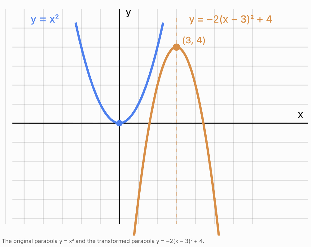
Comparing Different Orders of Transformations
Consider the parent function:
y = |x|
We will compare two transformation sequences.
Sequence A: Reflect, then translate upward
Reflect across the x-axis:
y = −|x|
Translate upward by 3:
y = −|x| + 3
The vertex is (0, 3).
Sequence B: Translate upward, then reflect
Translate upward by 3:
y = |x| + 3
Reflect across the x-axis:
y = −(|x| + 3)
y = −|x| − 3
The vertex is (0, −3).
The two graphs have different positions.
This demonstrates that reflection and translation do not always commute.
Two transformations commute when applying them in either order produces the same result.
Some transformations commute, while others do not.
For example, horizontal and vertical translations commute because they affect different coordinates.
Combining Transformations of Absolute Value Functions
Absolute value functions are useful for studying combined transformations because their V-shaped graphs have a clearly identifiable vertex.
The parent function is:
y = |x|
Consider:
y = −3|x + 2| + 5
Step 1: Identify the transformations
Compared with y = |x|:
-
Translate 2 units left.
-
Stretch vertically by a factor of 3.
-
Reflect across the x-axis.
-
Translate 5 units up.
Step 2: Identify the vertex
The parent vertex is (0, 0).
The new vertex is:
(−2, 5)
Because the coefficient is negative, the graph opens downward.
Step 3: Calculate key points
Use:
y = −3|x + 2| + 5
x
y
−4
−1
−3
2
−2
5
−1
2
0
−1
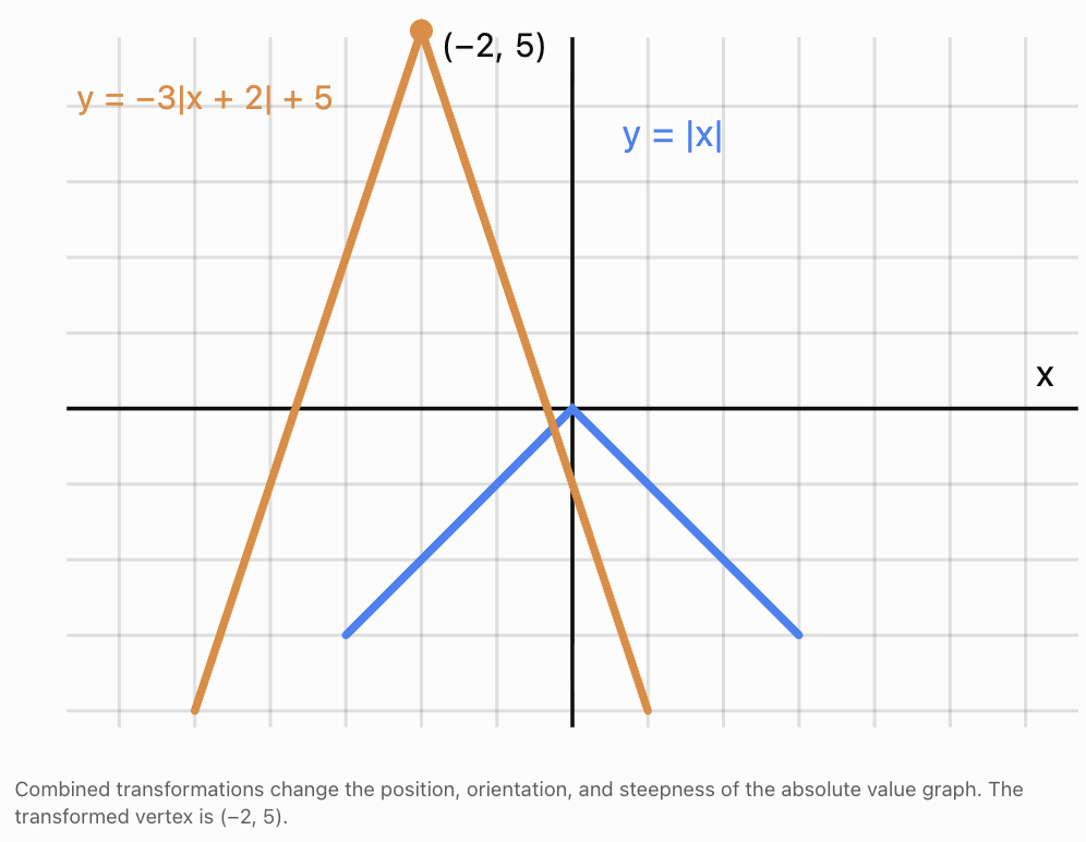
Combining Transformations of Square Root Functions
Consider the parent function:
y = √x
Its graph starts at (0, 0) and extends rightward and upward.
Now consider:
y = −2√(x − 4) + 3
Identify the transformations
-
Translate 4 units right.
-
Stretch vertically by a factor of 2.
-
Reflect across the x-axis.
-
Translate 3 units up.
Determine the starting point
The original starting point is (0, 0).
Using the coordinate rule:
(x, y) → (x + 4, −2y + 3)
The new starting point is:
(4, 3)
Transform other points
Original point
Transformed point
(0, 0)
(4, 3)
(1, 1)
(5, 1)
(4, 2)
(8, −1)
(9, 3)
(13, −3)
Domain and range
For the square root to be defined:
x − 4 ≥ 0
Therefore:
Domain: x ≥ 4
Because the square root is non-negative and multiplied by −2:
−2√(x − 4) ≤ 0
Adding 3:
Range: y ≤ 3
The transformed graph starts at (4, 3) and curves downward to the right.
Combining Horizontal and Vertical Scaling
When a function contains coefficients both inside and outside its expression, we must distinguish horizontal and vertical scaling.
Consider:
g(x) = 2f(3x)
The transformations are:
-
Horizontal compression by a factor of 1/3.
-
Vertical stretch by a factor of 2.
The coordinate rule is:
(x, y) → (x/3, 2y)
For example, if the original function contains the point (6, 4), the transformed point is:
(6/3, 2 × 4)
(2, 8)
Worked Example: Including translations
Consider:
g(x) = 3f(2(x − 4)) − 5
Identify the parameters:
a = 3
b = 2
h = 4
k = −5
Therefore:
-
Horizontal compression by a factor of 1/2.
-
Translation 4 units right.
-
Vertical stretch by a factor of 3.
-
Translation 5 units down.
Coordinate rule:
(x, y) → (x/2 + 4, 3y − 5)
If the parent function contains the point (2, 3):
x′ = 2/2 + 4 = 5
y′ = 3(3) − 5 = 4
The transformed point is:
(5, 4)
Why brackets matter
Compare:
g(x) = f(2(x − 4))
and:
g(x) = f(2x − 4)
The first can be read as a horizontal compression by 1/2 followed by a translation 4 units right.
The second can be rewritten as:
g(x) = f(2(x − 2))
It represents a horizontal compression by 1/2 followed by a translation 2 units right.
The two equations do not describe the same transformation.
Always factor the coefficient inside the function before identifying the horizontal translation.
Combining Transformations of Exponential Functions
Consider the parent function:
y = 2ˣ
Now consider:
y = −3(2⁽ˣ ⁻ ²⁾) + 4
Identify the transformations
-
Translate 2 units right.
-
Stretch vertically by a factor of 3.
-
Reflect across the x-axis.
-
Translate 4 units up.
Transform key points
The original function passes through:
(0, 1), (1, 2), (2, 4)
Apply:
(x, y) → (x + 2, −3y + 4)
Original point
Transformed point
(0, 1)
(2, 1)
(1, 2)
(3, −2)
(2, 4)
(4, −8)
Determine the asymptote
The original horizontal asymptote is:
y = 0
The vertical stretch and reflection leave this asymptote at y = 0.
The upward translation moves it to:
y = 4
The transformed graph approaches y = 4 from below.
Its domain is all real numbers, and its range is:
y < 4
Combining Transformations of Trigonometric Functions
Trigonometric functions often involve several transformations.
Consider:
y = 3 sin(2(x − π/4)) + 1
Compared with y = sin x:
-
Vertical stretch by a factor of 3.
-
Horizontal compression by a factor of 1/2.
-
Translation π/4 units right.
-
Translation 1 unit up.
The amplitude is:
3
The period is:
2π/2 = π
The midline is:
y = 1
The maximum value is:
1 + 3 = 4
The minimum value is:
1 − 3 = −2
These combined transformations are important in modeling sound waves, alternating electrical currents, vibrations, and periodic motion.
Identifying Transformations from Equations
A useful strategy is to compare the transformed equation with a familiar parent function.
Example A
y = 4(x + 3)² − 2
Compared with y = x²:
-
Vertical stretch by factor 4.
-
Translation 3 units left.
-
Translation 2 units down.
Example B
y = −0.5|x − 6| + 1
Compared with y = |x|:
-
Vertical compression by factor 0.5.
-
Reflection across the x-axis.
-
Translation 6 units right.
-
Translation 1 unit up.
Example C
y = √(2(x + 1)) − 4
Compared with y = √x:
-
Horizontal compression by factor 1/2.
-
Translation 1 unit left.
-
Translation 4 units down.
Example D
y = −2f(−3(x − 5)) + 7
Compared with y = f(x):
-
Horizontal compression by factor 1/3.
-
Reflection across the y-axis.
-
Translation 5 units right.
-
Vertical stretch by factor 2.
-
Reflection across the x-axis.
-
Translation 7 units up.
The corresponding coordinate rule is:
(x, y) → (−x/3 + 5, −2y + 7)
Comparing Multiple Transformed Graphs
Consider these three functions:
A: y = (x − 2)² + 3
B: y = 2(x − 2)² + 3
C: y = −0.5(x − 2)² + 3
All three have the same vertex:
(2, 3)
However, their shapes differ.
Feature
Graph A
Graph B
Graph C
Vertex
(2, 3)
(2, 3)
(2, 3)
Opens
Upward
Upward
Downward
Vertical scale
1
2
0.5
Width
Standard
Narrower
Wider
Extreme value
Minimum 3
Minimum 3
Maximum 3
Axis of symmetry
x = 2
x = 2
x = 2
This comparison shows how coefficients can change graph shape and orientation while leaving the vertex unchanged.
Sketching Combined Transformations
A reliable method for sketching transformed functions is to use key points from the parent graph.
Step 1: Identify the parent function
For example:
y = x²
Step 2: Identify the transformation parameters
Suppose:
y = −0.5(x + 2)² + 3
Then:
a = −0.5
h = −2
k = 3
Step 3: Write the coordinate rule
(x, y) → (x − 2, −0.5y + 3)
Step 4: Select key points
For y = x²:
(−2, 4), (−1, 1), (0, 0), (1, 1), (2, 4)
Step 5: Transform the points
Original
Transformed
(−2, 4)
(−4, 1)
(−1, 1)
(−3, 2.5)
(0, 0)
(−2, 3)
(1, 1)
(−1, 2.5)
(2, 4)
(0, 1)
Step 6: Draw and label the graph
The graph is a downward-opening parabola with:
-
Vertex (−2, 3).
-
Axis of symmetry x = −2.
-
Maximum value 3.
-
A wider shape than y = x².
Step 7: Verify the sketch
Substitute a few plotted x-values into the equation to confirm their y-values.
Determining an Equation from a Graph
Sometimes we are given the final graph and must work backwards to identify its equation.
Worked Example: Quadratic graph
A parabola has:
-
Vertex (3, −2).
-
Opens downward.
-
Passes through (4, −5).
Assume it has the form:
y = a(x − h)² + k
The vertex gives:
h = 3
k = −2
Therefore:
y = a(x − 3)² − 2
Use the point (4, −5):
−5 = a(4 − 3)² − 2
−5 = a − 2
a = −3
The equation is:
y = −3(x − 3)² − 2
Compared with y = x², this graph has:
-
Vertical stretch by factor 3.
-
Reflection across the x-axis.
-
Translation 3 units right.
-
Translation 2 units down.
Verification
At x = 4:
y = −3(1)² − 2
y = −5 ✓
Applications of Combined Transformations
Physics: Projectile motion
The height of a projectile may be modeled by:
h(t) = −5(t − 2)² + 25
This is a transformed quadratic function.
Compared with y = x²:
-
Vertical stretch by factor 5.
-
Reflection across the x-axis.
-
Translation 2 units right.
-
Translation 25 units up.
The vertex is:
(2, 25)
This means the projectile reaches a maximum height of 25 m after 2 seconds.
The equation can also be expanded:
h(t) = −5(t² − 4t + 4) + 25
h(t) = −5t² + 20t + 5
The initial height is 5 m.
Business: Revenue modeling
Suppose a company's revenue is modeled by:
R(x) = −2(x − 50)² + 5000
This parabola opens downward.
Its maximum occurs at:
x = 50
The maximum revenue is:
R = 5000
The vertex form makes it easy to identify the maximum without expanding the equation.
The vertical stretch factor determines how rapidly revenue decreases as x moves away from the optimal value.
Biology: Periodic measurements
Suppose a periodic biological measurement is modeled by:
P(t) = 5 sin(2(t − 1)) + 12
This model includes:
-
Vertical stretch by factor 5.
-
Horizontal compression by factor 1/2.
-
Translation 1 unit right.
-
Translation 12 units up.
The amplitude is 5.
The midline is 12.
The period is π time units.
The model's maximum value is 17, and its minimum value is 7.
This type of model can represent idealised rhythmic processes, although actual biological measurements may not follow perfect sine waves.
Evaluating Transformation Descriptions
A single transformed graph can sometimes be described using different combinations of transformations.
For example:
y = 4x²
Compared with y = x², this is a vertical stretch by factor 4.
But:
y = (2x)² = 4x²
Therefore, it can also be described as a horizontal compression by factor 1/2.
Both descriptions are valid.
Similarly, for exponential functions:
2(2ˣ) = 2⁽ˣ ⁺ ¹⁾
A vertical stretch by factor 2 produces the same graph as a translation 1 unit left.
The equation and parent function must be considered together when identifying transformations.
This is why different-looking transformation sequences can sometimes produce identical final graphs.
Common Mistakes
Applying transformations in the wrong order
A vertical stretch followed by a vertical translation may produce a different result from performing the translation first.
For example:
2(x² + 3) = 2x² + 6
is different from:
2x² + 3
Confusing horizontal translations
In y = f(x − 4), the graph moves 4 units right, not left.
Forgetting to factor horizontal coefficients
For:
y = f(3x − 6)
rewrite the input as:
3x − 6 = 3(x − 2)
The horizontal translation is 2 units right, not 6 units right.
Confusing vertical and horizontal scaling
In y = 3f(x), outputs are multiplied by 3.
In y = f(3x), horizontal distances are divided by 3.
Forgetting reflections
A negative coefficient outside a function introduces reflection across the x-axis.
A negative coefficient multiplying the input introduces reflection across the y-axis.
Moving the vertex without transforming other points
Every point must follow the same coordinate transformation rule.
Assuming all transformations change the graph visibly
Some functions have symmetries that make particular reflections leave the graph unchanged.
Ignoring domain and range restrictions
A transformed square root function may have a new starting point and different domain or range.
Confusing different but equivalent transformation descriptions
For some function families, horizontal scaling can produce the same graph as vertical scaling.
Failing to verify the final graph
Check key points, intercepts, turning points, asymptotes, and domain restrictions.
Key Terms
-
Combined transformation: Two or more transformations applied to a graph.
-
Parent function: A basic function used as the starting point for transformations.
-
Translation: A movement of a graph without changing its shape or orientation.
-
Reflection: A transformation producing a mirror image across a line.
-
Vertical stretch: Multiplying outputs by a factor greater than 1.
-
Vertical compression: Multiplying outputs by a positive factor less than 1.
-
Horizontal stretch: Increasing horizontal distances by a specified factor.
-
Horizontal compression: Decreasing horizontal distances by a specified factor.
-
Scale factor: A number describing how coordinates or distances are multiplied.
-
Coordinate transformation rule: A rule mapping original points to transformed points.
-
Vertex: A turning point of a parabola or the corner of an absolute value graph.
-
Axis of symmetry: A line dividing a graph into mirror-image halves.
-
Amplitude: The maximum displacement of a periodic function from its midline.
-
Period: The length of one complete cycle of a periodic function.
-
Midline: The central horizontal line around which a periodic function oscillates.
-
Domain: The set of permitted input values.
-
Range: The set of possible output values.
-
Asymptote: A line approached by a graph in a specified limiting direction.
-
Commutative transformations: Transformations that produce the same result when their order is reversed.
-
Equivalent transformations: Different transformation descriptions that produce the same final graph.
Key Takeaways
-
Combined transformations involve applying several changes to the same function.
-
The general form g(x) = af(b(x − h)) + k describes vertical and horizontal scaling, reflections, and translations.
-
The coordinate rule is (x, y) → (x/b + h, ay + k), where b ≠ 0.
-
The order of transformations can affect the final graph.
-
Horizontal and vertical scaling must be distinguished carefully.
-
Factoring expressions inside a function helps identify horizontal translations correctly.
-
Negative scaling coefficients can introduce reflections.
-
Vertices, endpoints, intercepts, and asymptotes are useful for sketching transformed graphs.
-
Domain and range restrictions may change under transformations.
-
Comparing transformed graphs helps reveal the effects of individual parameters.
-
Different transformation sequences can sometimes produce the same final function.
-
Verifying key points and features helps ensure accurate graph sketches.
Check Your Understanding
Recall and Understanding
1. What is meant by a combined transformation?
2. Explain why the order of transformations can affect the final graph.
3. State the coordinate transformation rule for g(x) = af(b(x − h)) + k.
4. Explain the difference between a vertical stretch by factor 3 and a horizontal compression by factor 1/3.
Application
5. Describe all transformations from y = x² to:
y = 3(x − 4)² + 2
6. Describe all transformations from y = |x| to:
y = −0.5|x + 3| − 2
7. The point (2, 5) undergoes the transformation:
(x, y) → (x + 4, −2y + 3)
Find its new coordinates.
8. Write the equation obtained by transforming y = x² using a vertical stretch by factor 2, a reflection across the x-axis, a translation 3 units left, and a translation 5 units up.
9. Determine the vertex, axis of symmetry, and range of:
y = −2(x − 1)² + 6
10. Describe the transformations represented by:
g(x) = 4f(2(x − 3)) − 1
Analysis and Challenge
11. A parabola has vertex (−2, 5), opens downward, and passes through (0, −3). Determine its equation in vertex form.
12. A student claims that y = 2(x² + 4) and y = 2x² + 4 represent the same transformation. Explain why this is incorrect.
13. Transform the points (−2, 4), (0, 0), and (2, 4) using:
g(x) = −3f(2(x − 1)) + 5
14. Compare the graphs:
A: y = (x − 2)² + 1
B: y = −2(x − 2)² + 1
Describe their similarities and differences.
15. The function y = √x is transformed into:
y = −2√(x + 4) + 3
Describe the transformations, state the starting point, and determine the domain and range.
Answers to Check Your Understanding
1. A combined transformation involves applying two or more transformations, such as translations, reflections, stretches, or compressions, to the same graph.
2. Transformations can affect the positions of points differently depending on their order. For example, stretching a graph vertically after translating it upward also scales the translation distance, whereas stretching first and then translating does not.
3.
For:
g(x) = af(b(x − h)) + k
the coordinate rule is:
(x, y) → (x/b + h, ay + k)
where b ≠ 0.
4. A vertical stretch by factor 3 multiplies y-coordinates by 3. A horizontal compression by factor 1/3 divides x-coordinates by 3. These are different transformations, although they can sometimes produce the same graph for particular functions.
5.
From y = x² to y = 3(x − 4)² + 2:
-
Vertical stretch by factor 3.
-
Translation 4 units right.
-
Translation 2 units up.
Vertex: (4, 2).
6.
From y = |x| to y = −0.5|x + 3| − 2:
-
Vertical compression by factor 0.5.
-
Reflection across the x-axis.
-
Translation 3 units left.
-
Translation 2 units down.
Vertex: (−3, −2).
7.
(x, y) → (x + 4, −2y + 3)
For (2, 5):
x′ = 2 + 4 = 6
y′ = −2(5) + 3 = −7
Answer: (6, −7)
8.
Start with y = x².
Apply the stretch and reflection:
y = −2x²
Translate 3 units left:
y = −2(x + 3)²
Translate 5 units up:
y = −2(x + 3)² + 5
9.
Given:
y = −2(x − 1)² + 6
Vertex:
(1, 6)
Axis of symmetry:
x = 1
The parabola opens downward, so its maximum value is 6.
Range:
y ≤ 6
10.
g(x) = 4f(2(x − 3)) − 1
Transformations:
-
Horizontal compression by factor 1/2.
-
Translation 3 units right.
-
Vertical stretch by factor 4.
-
Translation 1 unit down.
11.
Use vertex form:
y = a(x − h)² + k
The vertex is (−2, 5), so:
y = a(x + 2)² + 5
Substitute (0, −3):
−3 = a(0 + 2)² + 5
−3 = 4a + 5
4a = −8
a = −2
Therefore:
y = −2(x + 2)² + 5
Verification:
At x = 0:
y = −2(2²) + 5 = −3 ✓
12.
The equations are:
y = 2(x² + 4)
and:
y = 2x² + 4
Expand the first equation:
y = 2x² + 8
The second equation is:
y = 2x² + 4
They differ by 4 vertical units.
In the first equation, the graph is translated upward by 4 and then stretched vertically by factor 2.
In the second, the graph is stretched vertically by factor 2 and then translated upward by 4.
The transformations do not produce the same graph.
13.
Given:
g(x) = −3f(2(x − 1)) + 5
Coordinate rule:
(x, y) → (x/2 + 1, −3y + 5)
For (−2, 4):
x′ = −2/2 + 1 = 0
y′ = −3(4) + 5 = −7
Result: (0, −7)
For (0, 0):
x′ = 0/2 + 1 = 1
y′ = −3(0) + 5 = 5
Result: (1, 5)
For (2, 4):
x′ = 2/2 + 1 = 2
y′ = −3(4) + 5 = −7
Result: (2, −7)
Transformed points: (0, −7), (1, 5), (2, −7)
14.
Graph A:
y = (x − 2)² + 1
Graph B:
y = −2(x − 2)² + 1
Similarities:
-
Both have vertex (2, 1).
-
Both have axis of symmetry x = 2.
-
Both have domain consisting of all real numbers.
Differences:
-
Graph A opens upward.
-
Graph B opens downward.
-
Graph B is vertically stretched by factor 2 compared with Graph A.
-
Graph A has a minimum value of 1.
-
Graph B has a maximum value of 1.
15.
Original:
y = √x
Transformed:
y = −2√(x + 4) + 3
Transformations:
-
Translation 4 units left.
-
Vertical stretch by factor 2.
-
Reflection across the x-axis.
-
Translation 3 units up.
Original starting point:
(0, 0)
New starting point:
(−4, 3)
Domain:
x + 4 ≥ 0
x ≥ −4
Range:
Because √(x + 4) ≥ 0:
−2√(x + 4) + 3 ≤ 3
y ≤ 3
Final Summary
Combining transformations allows us to construct and interpret complex functions using familiar mathematical operations.
The general form:
g(x) = af(b(x − h)) + k
provides a framework for understanding horizontal and vertical scaling, reflections, and translations.
By recognising the effects of each parameter, applying coordinate rules, and comparing key graph features, we can sketch transformed functions accurately and explain how they relate to their parent functions.
The most important skill is understanding how the transformations work together, rather than memorising isolated rules.
-
5. Applications of Transformations
Learning outcomes
- I can apply transformations to solve problems.
- I can recognize transformations in real-life graphs.
- I can model situations using transformed functions.
- I can explain why transformations are useful.
- I can analyze transformed graphs.
Introduction
Graph transformations are not simply techniques for moving or changing the shape of mathematical graphs. They are powerful tools for understanding and modeling real-world situations.
Many relationships in science, economics, engineering, biology, and technology can be represented using familiar mathematical functions. Instead of constructing a completely new model for every situation, we can often transform an existing function to describe new conditions.
For example, consider the quadratic function:
y = x²
This is a basic mathematical model with a U-shaped graph.
Now consider:
h(t) = −5(t − 2)² + 25
This transformed quadratic function could represent the height of a projectile over time.
The transformations tell us that:
-
The graph opens downward because of the negative coefficient.
-
The vertical scale is changed by a factor of 5.
-
The maximum height occurs at t = 2 seconds.
-
The maximum height is 25 metres.
By recognising the transformations, we can understand important features of the model without performing lengthy calculations.
In this topic, we will explore how transformations are used to solve problems, recognise patterns in real-world graphs, build mathematical models, and interpret the meaning of transformed functions.
Why Are Transformations Useful?
A transformation allows us to modify a familiar mathematical relationship to represent a different situation.
For example, suppose a business has a cost function:
C(x) = 12x
This represents a production cost of $12 per item.
If the business must also pay a fixed operating cost of $500, the new function becomes:
C(x) = 12x + 500
The graph is translated upward by 500 units.
We do not need to develop a completely new mathematical structure. We simply adjust the original function.
Transformations are useful because they allow us to:
-
Adapt existing models to new conditions.
-
Predict how graphs change when parameters change.
-
Compare different scenarios.
-
Identify maximum and minimum values.
-
Interpret shifts in time or position.
-
Understand changes in amplitude, scale, and growth.
-
Simplify mathematical calculations.
-
Make predictions using transformed functions.
Reviewing the Main Transformations
Consider a parent function:
y = f(x)
The main transformations are:
|
Transformation |
Equation |
Effect |
|---|---|---|
|
Vertical translation |
y = f(x) + k |
Moves graph up or down |
|
Horizontal translation |
y = f(x − h) |
Moves graph right or left |
|
Reflection across x-axis |
y = −f(x) |
Reverses output signs |
|
Reflection across y-axis |
y = f(−x) |
Reverses input signs |
|
Vertical stretch |
y = af(x), a > 1 |
Multiplies outputs by a |
|
Vertical compression |
y = af(x), 0 < a < 1 |
Reduces output magnitudes |
|
Horizontal stretch |
y = f(x/b), b > 1 |
Increases horizontal distances |
|
Horizontal compression |
y = f(bx), b > 1 |
Decreases horizontal distances |
These transformations can be combined to represent more complicated situations.
General transformation model
A useful general equation is:
g(x) = af(b(x − h)) + k
where:
-
a controls vertical scaling and possible reflection.
-
b controls horizontal scaling and possible reflection.
-
h controls horizontal translation.
-
k controls vertical translation.
The values of these parameters can often be interpreted directly in a real-world context.
Recognising Transformations in Real-Life Graphs
When examining a real-world graph, look for changes in its important features.
Ask:
-
Has the graph moved upward or downward?
-
Does the same event occur earlier or later?
-
Have the maximum and minimum values changed?
-
Has the graph become steeper or flatter?
-
Has the period of a repeating pattern changed?
-
Has the graph been reflected?
-
Has the general shape remained the same?
Example: Comparing two temperature models
Suppose the temperature in one location is modeled by:
T₁(t) = 8 sin(πt/12) + 25
A second location has the model:
T₂(t) = 8 sin(πt/12) + 29
The second function is:
T₂(t) = T₁(t) + 4
Therefore, the second temperature graph is translated vertically upward by 4°C.
The models have:
-
The same amplitude.
-
The same period.
-
The same timing of maximum and minimum temperatures.
-
Different average temperatures.
The second location is modeled as being 4°C warmer at every corresponding time.
This is a simple example of how a vertical translation can represent a real-world difference.
Application: Projectile Motion
Projectile motion is one of the clearest applications of transformed quadratic functions.
When an object moves vertically under approximately constant gravitational acceleration, its height can be modeled by:
h(t) = h₀ + v₀t − ½gt²
where:
-
h(t) = height at time t.
-
h₀ = initial height.
-
v₀ = initial vertical velocity.
-
g = gravitational field strength.
-
t = time.
Near Earth's surface, g is approximately 9.8 m/s².
This equation is quadratic because it contains t².
Worked Example: A ball thrown upward
A ball is thrown upward from a platform 5 m above the ground with an initial vertical velocity of 20 m/s.
Using g = 10 m/s² for simplicity:
h(t) = 5 + 20t − 5t²
Rearrange:
h(t) = −5t² + 20t + 5
Step 1: Write in vertex form
Factor −5 from the quadratic terms:
h(t) = −5(t² − 4t) + 5
Complete the square:
t² − 4t = (t − 2)² − 4
Therefore:
h(t) = −5[(t − 2)² − 4] + 5
Expand:
h(t) = −5(t − 2)² + 25
Step 2: Interpret the transformations
Compared with y = x²:
-
Reflect across the x-axis.
-
Stretch vertically by a factor of 5.
-
Translate 2 units right.
-
Translate 25 units up.
Step 3: Identify the maximum height
The vertex is:
(2, 25)
Therefore:
Maximum height = 25 m
Time to maximum height = 2 s
Step 4: Find when the ball reaches the ground
Set h(t) = 0:
−5t² + 20t + 5 = 0
Divide by −5:
t² − 4t − 1 = 0
Apply the quadratic formula:
t = (4 ± √(16 + 4))/2
t = (4 ± √20)/2
t = 2 ± √5
The positive solution is:
t ≈ 4.24 s
The negative solution is not relevant because the model begins at t = 0.
The ball reaches the ground after approximately 4.24 seconds.
Why transformations are useful here
The vertex form makes the maximum height and its timing immediately visible.
We can also compare different launch conditions by examining how the parameters change.
For example, increasing the initial height while keeping the initial velocity unchanged translates the height-time graph upward.
Application: Business Revenue and Profit
Quadratic transformations are useful for modeling revenue and profit when these quantities depend on price or production.
Worked Example: Maximum profit
Suppose a business models its monthly profit using:
P(x) = −2(x − 40)² + 3200
where:
-
x = number of products sold, measured in hundreds.
-
P(x) = monthly profit in dollars.
Step 1: Identify the parent function
The parent function is:
y = x²
Step 2: Identify the transformations
The profit function has:
-
A reflection across the x-axis.
-
A vertical stretch by a factor of 2.
-
A horizontal translation 40 units right.
-
A vertical translation 3200 units up.
Step 3: Interpret the vertex
The vertex is:
(40, 3200)
Therefore:
Maximum modeled profit = $3,200
This occurs when x = 40, corresponding to 4,000 products sold.
Step 4: Compare different sales levels
At x = 30:
P(30) = −2(30 − 40)² + 3200
P(30) = −200 + 3200
P(30) = $3,000
At x = 50:
P(50) = −2(50 − 40)² + 3200
P(50) = $3,000
The model is symmetric about x = 40.
Interpretation
Selling 3,000 or 5,000 products gives the same modeled profit of $3,000.
The model suggests that profit decreases when sales move away from the optimal level.
This is an illustrative model; real business profit relationships may be more complicated.
Application: Comparing Production Costs
Linear functions are frequently used to model production costs.
Suppose a company has:
C₁(x) = 15x + 400
where:
-
x = number of products.
-
C₁(x) = total cost in dollars.
Now suppose the fixed operating cost increases by $200.
The new function becomes:
C₂(x) = 15x + 600
This is a vertical translation upward by 200 units.
Comparing the graphs
Both functions have gradient 15.
Therefore, the cost per additional product remains $15.
However, the second graph has a y-intercept of 600 instead of 400.
The difference between the functions is:
C₂(x) − C₁(x) = 200
This means the second production system costs $200 more at every production level.
Extension: Increasing variable costs
Suppose the variable cost increases from $15 to $18 per item, while the fixed cost stays at $400.
The new function is:
C₃(x) = 18x + 400
The gradient increases.
The graphs share the same y-intercept, but C₃(x) rises more quickly.
This is not a pure vertical stretch of the entire original function C₁(x), because a vertical stretch would also multiply the fixed cost.
Recognising this distinction is important when interpreting real-world models.
Application: Population Growth
Exponential functions are useful for modeling growth processes.
Suppose a population is modeled by:
P(t) = 500(1.08)ᵗ
where t is time in years.
The population begins at 500 and grows by 8% per year.
Scenario A: Doubling the initial population
If the initial population doubles but the growth rate remains unchanged:
P₂(t) = 1000(1.08)ᵗ
This can be written as:
P₂(t) = 2P(t)
The new graph is a vertical stretch by a factor of 2.
At every time t, the population is twice the original modeled population.
Scenario B: Growth begins 3 years later
Suppose the same growth pattern is delayed by 3 years.
A shifted model is:
P₃(t) = 500(1.08)⁽ᵗ ⁻ ³⁾
This is a horizontal translation 3 years to the right.
However, the model must be interpreted carefully.
If population growth is intended to begin only at t = 3, the shifted exponential model should be used for t ≥ 3, with the earlier period described separately.
Why transformations are useful
Transformations allow us to compare:
-
Different starting populations.
-
Different starting times.
-
Different measurement scales.
-
Growth patterns under different assumptions.
Application: Sound Waves and Oscillations
Many physical systems involve repeating patterns.
Examples include:
-
Sound waves.
-
Vibrating springs.
-
Pendulums at small angles.
-
Alternating electrical currents.
-
Rotating machinery.
These patterns can often be modeled using sine and cosine functions.
The general form is:
y = A sin(B(t − C)) + D
where:
-
A controls amplitude and possible reflection.
-
B controls the period.
-
C controls horizontal translation, or phase shift.
-
D controls vertical translation.
The amplitude is:
|A|
The period is:
2π/|B|
for B ≠ 0.
Worked Example: A vibrating object
Suppose the displacement of a vibrating object is:
y = 4 sin(2πt) + 1
where y is measured in centimetres and t in seconds.
Step 1: Identify the amplitude
A = 4
Therefore:
Amplitude = 4 cm
Step 2: Identify the period
B = 2π
Period = 2π/(2π)
Period = 1 s
Step 3: Identify the vertical translation
D = 1
The graph is translated upward by 1 cm.
Its midline is:
y = 1
Step 4: Determine maximum and minimum displacement
Maximum:
1 + 4 = 5 cm
Minimum:
1 − 4 = −3 cm
Interpretation
The object oscillates around a position 1 cm above the original reference level.
Its maximum displacement from that midline is 4 cm.
It completes one full cycle every second.
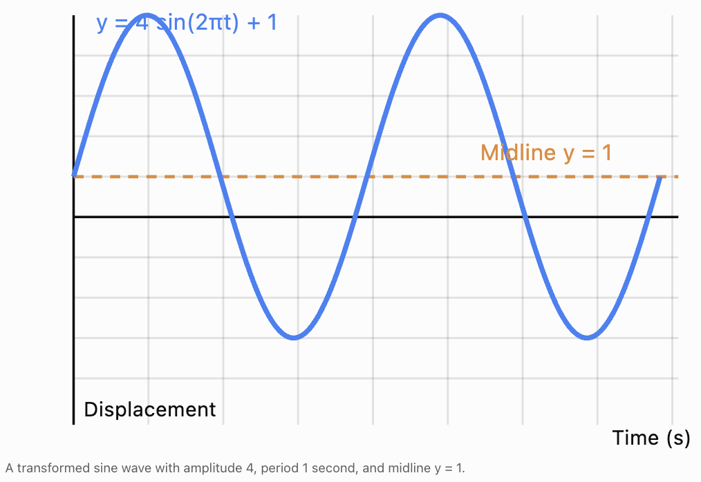
Application: Electrical Signals
Electronic signals can be modified using transformations.
Suppose an electrical signal is represented by:
V(t) = 2 sin(100πt)
where V is voltage in volts and t is time in seconds.
Increasing the amplitude
If the signal is amplified by a factor of 3:
V₂(t) = 6 sin(100πt)
This is a vertical stretch by a factor of 3.
The amplitude increases from 2 V to 6 V.
Introducing a time delay
If the signal is delayed by 0.005 seconds:
V₃(t) = 2 sin[100π(t − 0.005)]
This is a horizontal translation 0.005 seconds to the right.
Reversing polarity
If the signal's polarity is reversed:
V₄(t) = −2 sin(100πt)
This is a reflection across the horizontal axis.
Why transformations are useful
Engineers use these mathematical ideas to understand:
-
Signal amplification.
-
Time delays.
-
Phase differences.
-
Signal inversion.
-
Changes in frequency.
Application: Medical and Biological Signals
Some biological processes produce repeating electrical or mechanical patterns.
Examples include heartbeats, breathing cycles, and certain neural signals.
A simplified periodic signal might be modeled by:
S(t) = 2 sin(π(t − 1)) + 5
Compared with y = sin t:
-
Vertical stretch by factor 2.
-
Horizontal compression by factor 1/π.
-
Translation 1 time unit right.
-
Translation 5 units up.
The midline is 5.
The amplitude is 2.
The period is:
2π/π = 2 time units.
Real biological signals are often more complex than simple sine waves, but transformed functions can help describe basic features such as amplitude, timing, and frequency.
Application: Transformations in Geometry and Computer Graphics
Transformations are widely used in computer graphics, animation, engineering design, and digital mapping.
A point in a two-dimensional coordinate system can be transformed using coordinate rules.
Translation
Move a point h units horizontally and k units vertically:
(x, y) → (x + h, y + k)
Reflection across the x-axis
(x, y) → (x, −y)
Reflection across the y-axis
(x, y) → (−x, y)
Vertical scaling
(x, y) → (x, ay)
Horizontal scaling
(x, y) → (bx, y)
Worked Example: Transforming a digital shape
A triangle has vertices:
A(1, 2)
B(3, 2)
C(2, 5)
The triangle undergoes:
-
A horizontal translation 4 units right.
-
A vertical stretch by factor 2.
-
A reflection across the x-axis.
Step 1: Write the coordinate rule
The combined rule is:
(x, y) → (x + 4, −2y)
Step 2: Transform each vertex
A(1, 2):
A′ = (5, −4)
B(3, 2):
B′ = (7, −4)
C(2, 5):
C′ = (6, −10)
Step 3: Interpret the result
The triangle has moved right, become twice as tall, and been reflected vertically.
Unlike a pure translation or reflection, the vertical stretch changes its shape.
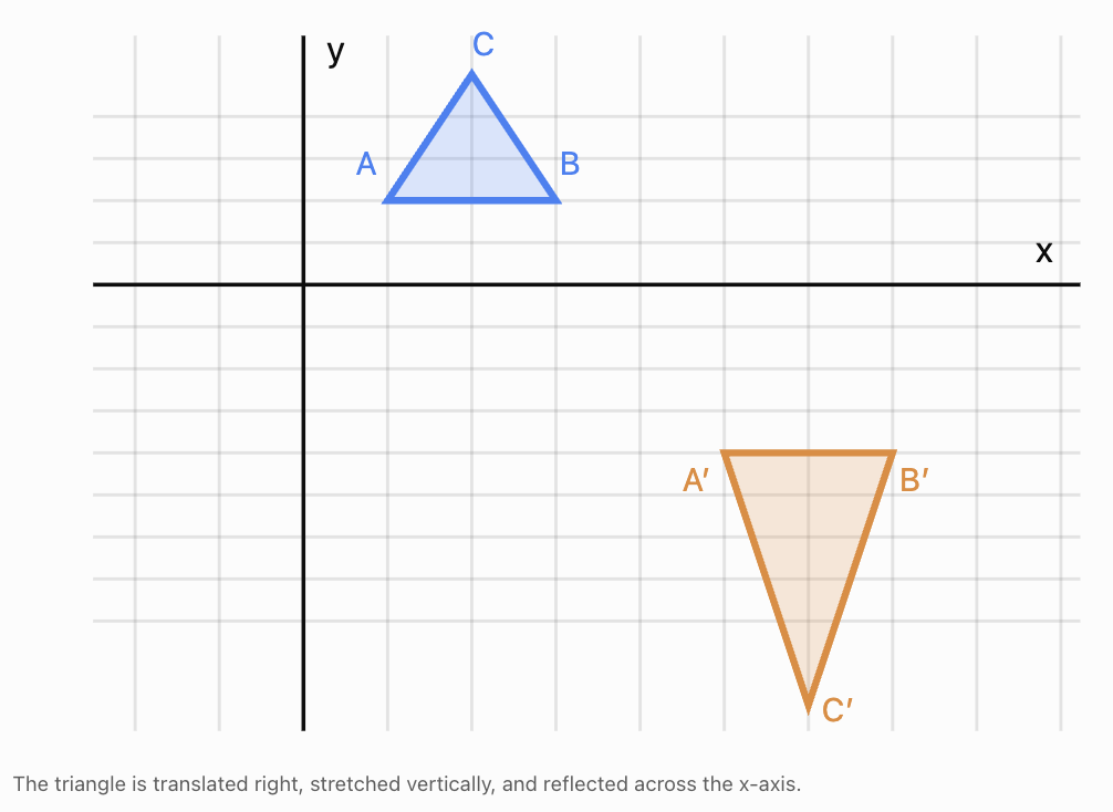
Modeling Real Situations Using Transformed Functions
When building a mathematical model, begin by identifying the general shape of the relationship.
Step 1: Identify the parent function
Ask whether the situation resembles:
-
A straight line.
-
A parabola.
-
An exponential curve.
-
A square root curve.
-
A periodic sine or cosine wave.
Step 2: Identify important features
These might include:
-
Starting value.
-
Maximum or minimum.
-
Time of an important event.
-
Rate of change.
-
Amplitude.
-
Period.
-
Long-term behaviour.
Step 3: Select transformations
Use translations, stretches, compressions, or reflections to match the required features.
Step 4: Construct the equation
For example, a quadratic model can be written:
y = a(x − h)² + k
The vertex is (h, k).
The value of a controls the vertical scale and direction of opening.
Step 5: Verify the model
Substitute known data points and check whether the model satisfies the conditions.
Step 6: Evaluate limitations
A mathematical model is a simplified representation of reality.
Its accuracy depends on the assumptions and the range of values for which it is used.
Worked Example: Building a Quadratic Model
A water fountain produces an arch of water.
The water reaches a maximum height of 4 m at a horizontal distance of 2 m from the nozzle.
The nozzle is located at ground level.
Find a quadratic equation modeling the height of the water.
Step 1: Choose the model
Use vertex form:
h(x) = a(x − p)² + q
The vertex is (2, 4).
Therefore:
h(x) = a(x − 2)² + 4
Step 2: Use the starting point
The water begins at (0, 0).
Substitute:
0 = a(0 − 2)² + 4
0 = 4a + 4
a = −1
Step 3: Write the equation
h(x) = −(x − 2)² + 4
Step 4: Determine where the water lands
Set h(x) = 0:
0 = −(x − 2)² + 4
(x − 2)² = 4
x − 2 = ±2
x = 0 or x = 4
The water returns to ground level at:
x = 4 m
Interpretation
The water travels 4 m horizontally from the nozzle before returning to the ground.
The model assumes an ideal parabolic trajectory and ignores air resistance and other effects.
Analyzing Transformed Graphs
When analyzing a transformed graph, consider the following questions.
What is the parent function?
Identify the familiar graph shape.
Which transformations have occurred?
Look for translations, reflections, stretches, and compressions.
What are the important features?
Determine vertices, intercepts, asymptotes, maxima, minima, and other significant points.
What do the parameters mean?
Relate each parameter to the real-world situation.
What are the domain and range?
Identify the mathematically permitted values and the values that make sense in context.
What predictions can the model make?
Use the equation to calculate unknown values.
What are the model's limitations?
Consider whether the assumptions remain reasonable outside the observed data.
Example: Interpreting a transformed graph
Suppose a model is:
y = −3(x − 5)² + 75
We can immediately identify:
-
Parent function: y = x².
-
Reflection across the x-axis.
-
Vertical stretch by factor 3.
-
Translation 5 units right.
-
Translation 75 units up.
-
Vertex: (5, 75).
-
Maximum value: 75.
-
Axis of symmetry: x = 5.
If y represents height, this might describe an object reaching a maximum height of 75 units when x = 5.
If y represents profit, it might describe a maximum profit of 75 units at an input value of 5.
The mathematical structure is the same, but the interpretation depends on the context.
Comparing Multiple Transformed Models
Suppose three objects follow these height models:
A: h(t) = −5(t − 2)² + 20
B: h(t) = −5(t − 2)² + 30
C: h(t) = −10(t − 2)² + 20
Comparing A and B
Model B is a vertical translation of Model A upward by 10 m.
Both objects:
-
Reach their maximum height at t = 2 s.
-
Have the same quadratic coefficient.
-
Have the same curvature.
However, Model B is always 10 m higher than Model A at corresponding times.
Comparing A and C
Model C has a quadratic coefficient of −10 rather than −5.
Compared with Model A, its vertical deviations from the shared maximum height of 20 m are doubled.
Model C therefore has a narrower parabola.
Both models have their maximum at:
(2, 20)
However, Model C decreases more rapidly as t moves away from 2.
Comparison table
|
Feature |
Model A |
Model B |
Model C |
|---|---|---|---|
|
Maximum height |
20 m |
30 m |
20 m |
|
Time of maximum |
2 s |
2 s |
2 s |
|
Quadratic coefficient |
−5 |
−5 |
−10 |
|
Graph width |
Standard relative to A |
Same as A |
Narrower |
|
Axis of symmetry |
t = 2 |
t = 2 |
t = 2 |
This comparison shows how transformed equations allow us to understand several models without plotting every point.
Evaluating the Usefulness of Transformations
Transformations are particularly valuable when we want to compare models that share a common mathematical structure.
They can help us:
-
Identify changes quickly.
-
Reduce the amount of calculation required.
-
Explain differences between related situations.
-
Estimate important values.
-
Predict the effects of changing parameters.
-
Communicate mathematical relationships clearly.
However, transformations do not guarantee that a model accurately represents reality.
A good model must also be supported by appropriate assumptions and data.
For example, a transformed quadratic may accurately describe the short-term motion of a projectile, but it may not be suitable for modeling the entire flight of an object experiencing significant air resistance.
Similarly, an exponential growth model may work over a limited period but become unrealistic when resources are limited.
Common Mistakes
Confusing mathematical transformations with real-world changes
A vertical translation represents adding the same amount to every output. Not every real-world increase is a vertical translation.
Ignoring units
A vertical shift of 5 might represent 5 metres, 5 dollars, or 5°C depending on the context.
Misinterpreting the vertex
In a quadratic model, the vertex may represent a maximum or minimum. Its meaning depends on the situation.
Confusing stretches with translations
Multiplying outputs changes their scale, while adding a constant shifts them vertically.
Forgetting horizontal translation directions
In f(x − 3), the graph moves 3 units right.
Using unrealistic domains
A time model may be mathematically defined for negative values, but negative time may not be meaningful in the problem.
Assuming a model is valid indefinitely
Real-world relationships often have practical limits.
Failing to check the equation against known data
A model should reproduce the given conditions.
Assuming every parameter has an independent physical meaning
Some mathematical transformations can be described in different ways. The interpretation should be supported by the context.
Key Terms
-
Transformation: A change to the position, orientation, or scale of a graph.
-
Mathematical model: An equation or mathematical relationship representing a real-world situation.
-
Parent function: A basic function used as the starting point for transformations.
-
Translation: A transformation moving a graph horizontally or vertically.
-
Reflection: A transformation producing a mirror image across a line.
-
Vertical stretch: Multiplying all outputs by a factor greater than 1.
-
Vertical compression: Multiplying all outputs by a positive factor less than 1.
-
Horizontal stretch: Increasing horizontal distances by a scale factor.
-
Horizontal compression: Decreasing horizontal distances by a scale factor.
-
Scale factor: A multiplier describing how coordinates or distances change.
-
Vertex: The turning point of a parabola.
-
Maximum value: The greatest output of a function over its specified domain.
-
Minimum value: The smallest output of a function over its specified domain.
-
Amplitude: The maximum displacement of a periodic function from its midline.
-
Period: The interval required for one complete cycle.
-
Phase shift: A horizontal translation of a periodic function.
-
Midline: The central horizontal line around which a periodic function oscillates.
-
Domain: The set of allowed input values.
-
Range: The set of possible output values.
-
Asymptote: A line approached by a graph in a specified limiting direction.
-
Model assumptions: Conditions accepted as true when constructing a mathematical model.
-
Model limitations: Factors restricting how accurately or widely a model can be applied.
Key Takeaways
-
Graph transformations are useful for adapting mathematical models to new situations.
-
Vertical translations can represent fixed increases or decreases.
-
Horizontal translations can represent time delays or shifts in position.
-
Vertical stretches and compressions can represent changes in amplitude or scale.
-
Reflections can represent changes in direction or sign.
-
Quadratic transformations help identify maximum and minimum values.
-
Exponential transformations help compare growth processes.
-
Trigonometric transformations help model periodic phenomena.
-
Transformations allow related models to be compared efficiently.
-
Real-world interpretation requires attention to units, domains, and assumptions.
-
Mathematical models should be verified using known information.
-
The usefulness of a transformed function depends on how well it represents the situation being studied.
Check Your Understanding
Recall and Understanding
1. Explain why graph transformations are useful in mathematical modeling.
2. Give a real-world example of a vertical translation.
3. Explain how a horizontal translation might represent a time delay.
4. Describe the difference between increasing the amplitude and increasing the frequency of a periodic function.
Application
5. A company's cost function is C(x) = 20x + 300. Fixed costs increase by $150. Write the new cost function and describe the transformation.
6. A population is modeled by P(t) = 400(1.05)ᵗ. The initial population doubles while the growth rate remains unchanged. Write the new function.
7. A vibrating object has displacement y = 3 sin(2πt). Its amplitude increases by a factor of 2. Write the new equation and state its amplitude.
8. A quadratic function is given by h(t) = −5(t − 3)² + 45. Determine the maximum height and the time at which it occurs.
9. A business models profit using P(x) = −4(x − 20)² + 2000. Determine the maximum profit and the value of x at which it occurs.
10. A signal is represented by V(t) = 5 sin(10t). Write the equation after a reflection across the horizontal axis.
Analysis and Challenge
11. A ball is thrown upward from ground level with an initial vertical velocity of 30 m/s. Using g = 10 m/s², construct a quadratic height model and determine its maximum height.
12. A fountain produces a parabolic water arc with a maximum height of 6 m at a horizontal distance of 3 m from the nozzle. The water begins at ground level. Find an equation for the arc and determine where the water lands.
13. Compare the functions:
A: y = −2(x − 4)² + 30
B: y = −2(x − 4)² + 40
C: y = −4(x − 4)² + 30
Describe the transformations and compare their maximum values.
14. A periodic function is modeled by y = 5 sin(π(t − 2)) + 10. Determine its amplitude, period, phase shift, midline, maximum, and minimum.
15. A student claims that doubling the fixed costs of a business always produces a vertical stretch of its total cost graph. Explain why this is incorrect.
Answers to Check Your Understanding
1. Transformations allow familiar functions to be adapted to new situations without constructing completely new models. They help us interpret changes, compare scenarios, and make predictions.
2. An increase in a company's fixed operating costs adds the same amount to the total cost at every production level, producing a vertical translation upward.
3. Replacing f(t) with f(t − h), where h > 0, moves the graph h time units to the right. This can represent an event occurring later.
4. Increasing amplitude changes the maximum displacement from the midline. Increasing frequency increases the number of cycles per unit time and decreases the period.
5.
Original:
C(x) = 20x + 300
New fixed cost:
300 + 150 = 450
C(x) = 20x + 450
Transformation: Vertical translation upward by 150.
6.
Original:
P(t) = 400(1.05)ᵗ
Double the initial population:
P₂(t) = 800(1.05)ᵗ
This is a vertical stretch by factor 2.
7.
Original:
y = 3 sin(2πt)
Double the amplitude:
y = 6 sin(2πt)
Amplitude = 6.
8.
h(t) = −5(t − 3)² + 45
Vertex:
(3, 45)
Maximum height = 45 m
Time = 3 s
9.
P(x) = −4(x − 20)² + 2000
Vertex:
(20, 2000)
Maximum profit = $2,000
This occurs at x = 20.
10.
Original:
V(t) = 5 sin(10t)
Reflection across the horizontal axis:
V(t) = −5 sin(10t)
11.
Use:
h(t) = v₀t − ½gt²
Substitute:
h(t) = 30t − 5t²
Complete the square:
h(t) = −5(t² − 6t)
h(t) = −5[(t − 3)² − 9]
h(t) = −5(t − 3)² + 45
Vertex:
(3, 45)
Maximum height = 45 m
This occurs after 3 seconds.
12.
Use vertex form:
h(x) = a(x − 3)² + 6
The water begins at (0, 0).
Substitute:
0 = a(0 − 3)² + 6
0 = 9a + 6
a = −6/9 = −2/3
Therefore:
h(x) = −(2/3)(x − 3)² + 6
To find where the water lands:
0 = −(2/3)(x − 3)² + 6
(2/3)(x − 3)² = 6
(x − 3)² = 9
x − 3 = ±3
x = 0 or x = 6
The water lands at:
x = 6 m
13.
Model A:
y = −2(x − 4)² + 30
Maximum = 30 at x = 4.
Model B:
y = −2(x − 4)² + 40
Maximum = 40 at x = 4.
Model C:
y = −4(x − 4)² + 30
Maximum = 30 at x = 4.
Comparison:
-
B is A translated upward by 10 units.
-
C has the same vertex as A but is vertically stretched by factor 2 relative to its vertex level, making it narrower.
-
All three graphs open downward.
-
All three have their maximum at x = 4.
14.
Given:
y = 5 sin(π(t − 2)) + 10
Amplitude:
5
Period:
2π/π = 2
Phase shift:
2 units right
Midline:
y = 10
Maximum:
10 + 5 = 15
Minimum:
10 − 5 = 5
15.
Doubling fixed costs changes the constant term of a cost function, not necessarily every output by the same factor.
For example:
Original:
C(x) = 10x + 200
Doubling fixed costs:
C₂(x) = 10x + 400
This is a vertical translation upward by 200.
A vertical stretch by factor 2 would instead give:
2C(x) = 20x + 400
This doubles both the variable cost and the fixed cost.
Therefore, doubling fixed costs does not generally produce a vertical stretch of the total cost graph.
Final Summary
Applications of transformations demonstrate how familiar mathematical functions can be adapted to represent real-world situations.
Translations can model shifts in position, time, or baseline values. Stretches and compressions can represent changes in scale or amplitude. Reflections can represent reversals in direction or sign.
By recognising these transformations, we can construct models, compare different scenarios, identify important graph features, and make useful predictions.
The central idea is that understanding how a function changes is often just as important as knowing the function itself.