Transformations of Graphs

Introduction

Not all graph transformations involve moving a graph to a different position or reflecting it across an axis. Some transformations change the graph's shape by stretching or compressing it.

A stretch makes a graph larger in a particular direction, while a compression makes it smaller in that direction.

For example, consider the quadratic function:

y = x²

Its graph is a parabola with a vertex at (0, 0).

Now consider:

y = 3x²

For every value of x, the output is three times the original output. This is called a vertical stretch by a factor of 3.

Alternatively:

y = 0.5x²

Every output is half its original value. This is a vertical compression by a factor of 0.5.

These transformations are important because they allow us to change the shape of a graph while preserving its general mathematical structure.

Stretches and compressions appear in quadratic functions, absolute value functions, exponential functions, trigonometric functions, and many mathematical models used in science and engineering.

What Are Stretches and Compressions?

A stretch or compression is a transformation that changes the distance of points from a particular axis.

There are two main types:

• Vertical stretches and compressions: Change the y-coordinates of points.

• Horizontal stretches and compressions: Change the x-coordinates of points.

In this topic, our main focus is on vertical transformations, although horizontal transformations will also be introduced for comparison.

Unlike translations and reflections, stretches and compressions generally change the shape or dimensions of a graph.

However, some points may remain unchanged, especially points lying on the relevant axis.

Vertical Stretches

A vertical stretch moves points farther from the x-axis.

For an original function:

y = f(x)

A vertical stretch by a factor of a is represented by:

y = af(x)

where:

a > 1

Every y-coordinate is multiplied by a.

The x-coordinates remain unchanged.

Coordinate rule

(x, y) → (x, ay)

For example, a vertical stretch by a factor of 3 transforms:

• (1, 2) → (1, 6)

• (2, 4) → (2, 12)

• (−1, −3) → (−1, −9)

• (0, 0) → (0, 0)

Points above the x-axis move farther upward.

Points below the x-axis move farther downward.

Points on the x-axis remain fixed.

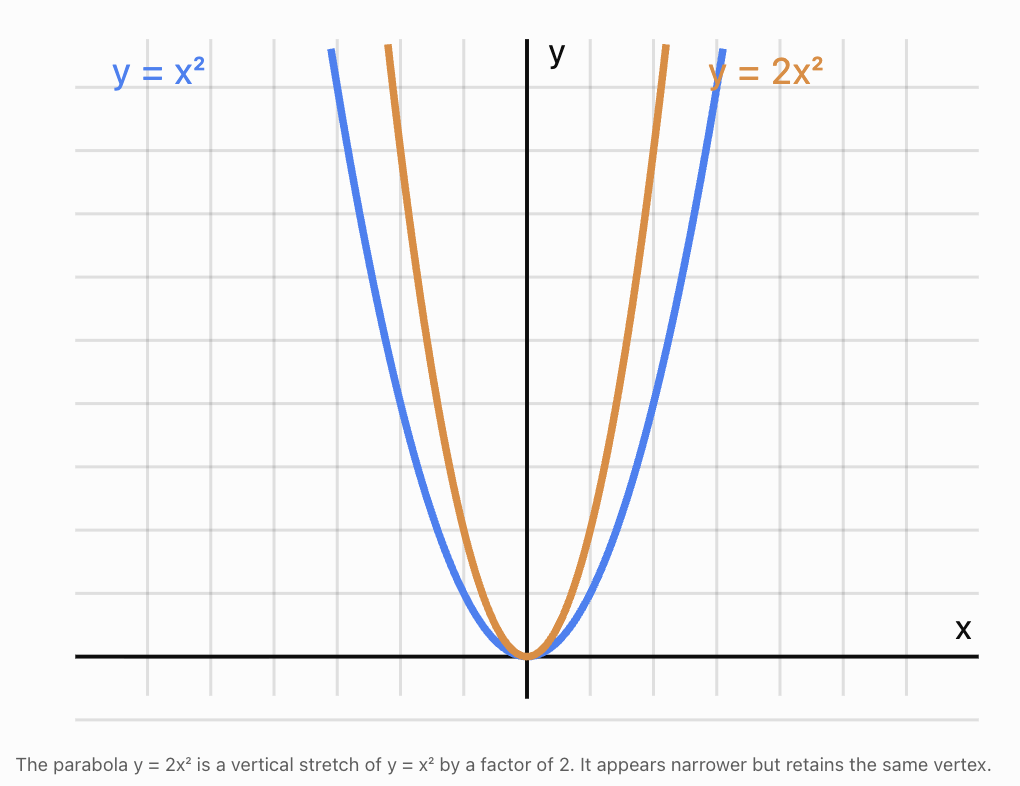
Worked Example: Vertical Stretch of a Quadratic Function

Original function:

y = x²

Transformed function:

y = 2x²

The transformed function is a vertical stretch by a factor of 2.

Compare the values:

Every output is doubled.

The vertex remains at (0, 0).

The transformed parabola appears narrower than the original because its height increases more quickly as we move away from the vertex.

Vertical Compressions

A vertical compression moves points closer to the x-axis.

For an original function:

y = f(x)

a vertical compression is represented by:

y = af(x)

where:

0 < a < 1

Every y-coordinate is multiplied by a number between 0 and 1.

Coordinate rule

(x, y) → (x, ay)

For example, a vertical compression by a factor of 0.5 transforms:

• (1, 6) → (1, 3)

• (2, 8) → (2, 4)

• (−1, −4) → (−1, −2)

• (0, 0) → (0, 0)

Points move closer to the x-axis.

Worked Example: Vertical Compression of a Quadratic Function

Original:

y = x²

Transformed:

y = 0.5x²

The transformed function is a vertical compression by a factor of 0.5.

The outputs are halved.

The parabola appears wider because it increases more slowly as x moves away from zero.

Comparing Vertical Stretches and Compressions

The coefficient outside a function determines the vertical scaling.

The absolute value of the coefficient determines the scale.

The sign determines whether an additional reflection occurs.

General rule

For:

y = af(x)

• |a| > 1: vertical stretch.

• 0 < |a| < 1: vertical compression.

• a < 0: reflection across the x-axis as well.

• a = 1: no vertical scaling.

• a = −1: reflection across the x-axis only.

• a = 0: all outputs become zero, collapsing the graph onto the x-axis over its domain.

Stretches and Compressions of Absolute Value Functions

Absolute value functions provide a clear visual example of vertical scaling.

The parent function is:

y = |x|

Its graph has a V-shape with a vertex at (0, 0).

Worked Example: Vertical stretch

Consider:

y = 3|x|

Every output is multiplied by 3.

The graph becomes steeper, and its V-shape appears narrower.

Worked Example: Vertical compression

Consider:

y = 0.25|x|

Every output is multiplied by 0.25.

The graph becomes less steep and appears wider.

For example, the original point (4, 4) becomes (4, 1).

The vertex remains at (0, 0).

Worked Example: Scaling and reflection

Consider:

y = −2|x|

The coefficient −2 produces two transformations:

• A vertical stretch by a factor of 2.

• A reflection across the x-axis.

The graph opens downward and is steeper than y = |x|.

Stretches and Compressions of Linear Functions

Vertical scaling also applies to straight lines.

Consider:

f(x) = 2x + 1

Apply a vertical stretch by a factor of 3:

g(x) = 3f(x)

g(x) = 3(2x + 1)

g(x) = 6x + 3

The original gradient is 2.

The transformed gradient is 6.

The original y-intercept is 1.

The transformed y-intercept is 3.

Both the gradient and the y-intercept are multiplied by 3.

Worked Example: Vertical compression

Original:

y = 4x − 8

Compress vertically by a factor of 0.5:

y = 0.5(4x − 8)

y = 2x − 4

The gradient decreases from 4 to 2.

The y-intercept changes from −8 to −4.

An important observation is that a vertical stretch or compression of a straight line can also be described as a change in its gradient and intercept. Unlike a parabola, a straight line does not become visibly narrower or wider.

Horizontal Stretches and Compressions

Although our main focus is vertical scaling, it is useful to compare vertical transformations with horizontal ones.

For a function:

y = f(x)

a horizontal scaling can be written:

y = f(bx)

where b is a nonzero constant.

The horizontal scale factor is:

1/|b|

For positive b:

• b > 1 produces a horizontal compression.

• 0 < b < 1 produces a horizontal stretch.

For negative b, there is also a reflection across the y-axis.

Example: Horizontal compression

Original:

y = x²

Transformed:

y = (2x)²

Simplify:

y = 4x²

The horizontal scale factor is 1/2.

This is a horizontal compression by a factor of 1/2.

Interestingly, for this particular function, the same resulting graph can be described as a vertical stretch by a factor of 4.

Example: Horizontal stretch

Original:

y = x²

Transformed:

y = (x/2)²

Simplify:

y = 0.25x²

The horizontal scale factor is 2.

This is a horizontal stretch by a factor of 2.

It is also equivalent to a vertical compression by a factor of 0.25 for this particular function.

Comparing vertical and horizontal scaling

Remember: A coefficient outside the function scales outputs. A coefficient multiplying the input scales horizontal distances by its reciprocal.

Identifying Transformations from Equations

We can often identify stretches and compressions simply by examining the equation.

Worked Example: Quadratic function

Consider:

y = 5x²

Compared with y = x², the coefficient is 5.

Since 5 > 1, the graph undergoes a vertical stretch by a factor of 5.

Worked Example: Absolute value function

Consider:

y = 0.2|x|

Since 0 < 0.2 < 1, the graph undergoes a vertical compression by a factor of 0.2.

Worked Example: Negative coefficient

Consider:

y = −0.5x²

The coefficient has an absolute value of 0.5.

Therefore, the graph undergoes:

• A vertical compression by a factor of 0.5.

• A reflection across the x-axis.

The parabola opens downward and appears wider than y = x².

Combining Scaling with Translations

Stretches and compressions can be combined with translations.

A useful general form is:

y = af(x − h) + k

where:

• a controls vertical scaling and possibly reflection.

• h controls horizontal translation.

• k controls vertical translation.

Worked Example: Quadratic transformation

Consider:

y = 2(x − 3)² + 4

Compared with y = x²:

• Vertical stretch by factor 2.

• Translation 3 units right.

• Translation 4 units up.

The vertex is:

(3, 4)

The parabola opens upward and is narrower than y = x².

Worked Example: Compression and translation

Consider:

y = 0.5(x + 2)² − 3

Compared with y = x²:

• Vertical compression by factor 0.5.

• Translation 2 units left.

• Translation 3 units down.

The vertex is:

(−2, −3)

The parabola opens upward and is wider than y = x².

Worked Example: Stretch, reflection, and translation

Consider:

y = −3|x − 1| + 5

Compared with y = |x|:

• Vertical stretch by factor 3.

• Reflection across the x-axis.

• Translation 1 unit right.

• Translation 5 units up.

The vertex is:

(1, 5)

The graph is an inverted V-shape.

Sketching Stretched and Compressed Graphs

A reliable sketching method uses key points.

Step 1: Identify the parent function

For example:

y = x²

Step 2: Identify the scale factor

Suppose the transformed function is:

y = 3x²

The vertical scale factor is 3.

Step 3: Choose key points

For the parent function:

(−2, 4), (−1, 1), (0, 0), (1, 1), (2, 4)

Step 4: Apply the coordinate rule

Multiply each y-coordinate by 3.

New points:

(−2, 12), (−1, 3), (0, 0), (1, 3), (2, 12)

Step 5: Plot the transformed points

Use the same coordinate scale for both graphs.

Step 6: Draw a smooth curve

The transformed graph should pass through the new points.

Step 7: Check the result

The new parabola should:

• Have the same vertex.

• Open upward.

• Be narrower than the original.

• Have outputs three times the original values.

Comparing Original and Transformed Graphs

When comparing graphs, examine their key features.

For quadratic functions, useful features include:

• Vertex.

• Axis of symmetry.

• Direction of opening.

• Width.

• Intercepts.

• Minimum or maximum value.

Worked Example

Compare:

y = x²

y = 4x²

y = 0.25x²

All three graphs:

• Have vertex (0, 0).

• Have axis of symmetry x = 0.

• Open upward.

• Have domain consisting of all real numbers.

• Have range y ≥ 0.

However:

• y = 4x² is narrower than y = x².

• y = 0.25x² is wider than y = x².

This demonstrates that vertical scaling can change a graph's appearance without changing its vertex or direction of opening.

Stretches and Compressions of Exponential Functions

Consider the parent function:

y = 2ˣ

Apply a vertical stretch by factor 3:

y = 3(2ˣ)

Every output is tripled.

For example:

At x = 0:

Original y = 1

Transformed y = 3

At x = 2:

Original y = 4

Transformed y = 12

The horizontal asymptote remains y = 0.

Vertical compression

Consider:

y = 0.5(2ˣ)

Every output is halved.

At x = 2:

Original y = 4

Transformed y = 2

The graph retains its exponential growth pattern.

For exponential functions, vertical scaling can sometimes also be expressed as a horizontal translation. For example:

2(2ˣ) = 2⁽ˣ ⁺ ¹⁾

The same graph can therefore have more than one valid transformation description.

Stretches and Compressions of Trigonometric Functions

Trigonometric functions provide an important application of vertical scaling.

Consider:

y = sin x

The maximum value is 1, and the minimum value is −1.

Its amplitude is 1.

Now consider:

y = 3 sin x

The maximum value becomes 3.

The minimum value becomes −3.

The amplitude is 3.

This is a vertical stretch by factor 3.

Vertical compression

Consider:

y = 0.5 sin x

The maximum value is 0.5.

The minimum value is −0.5.

The amplitude is 0.5.

This is a vertical compression by factor 0.5.

General trigonometric form

For:

y = a sin x

the amplitude is:

Amplitude = |a|

A negative value of a also reflects the graph across the x-axis.

For example:

y = −2 sin x

has amplitude 2 and is reflected across the x-axis compared with y = sin x.

Applications in Science and Engineering

Physics: Oscillations

A vibrating object may be modeled by:

y = A sin(ωt)

where:

• A = amplitude.

• ω = angular frequency.

• t = time.

Increasing A produces a vertical stretch.

Decreasing A produces a vertical compression.

For example:

y = 2 sin(3t)

has twice the amplitude of:

y = sin(3t)

The oscillation frequency remains unchanged.

Economics: Scaling revenue

Suppose a company's revenue is modeled by:

R(x) = 20x

If the selling price increases to $30 per unit, the new revenue function becomes:

R(x) = 30x

Since:

30x = 1.5(20x)

the new revenue graph is a vertical stretch of the original by a factor of 1.5.

This assumes the number of units sold remains the same at each value of x.

Biology: Comparing measurements

Suppose a laboratory instrument records a signal represented by:

S(t) = f(t)

If the signal is amplified threefold, the new signal is:

S(t) = 3f(t)

This is a vertical stretch by a factor of 3.

Signal amplification is common in scientific instruments, medical equipment, and electronic sensors.

Common Mistakes

Confusing stretches and compressions

A vertical stretch has a scale factor greater than 1.

A vertical compression has a scale factor between 0 and 1.

Confusing vertical and horizontal scaling

In y = 3f(x), the outputs are multiplied by 3.

In y = f(3x), horizontal distances are divided by 3.

Assuming a negative coefficient only produces scaling

A negative coefficient outside the function also produces reflection across the x-axis.

Multiplying x-coordinates during a vertical stretch

Vertical scaling changes y-coordinates, not x-coordinates.

Changing the vertex incorrectly

For y = ax², the vertex remains at (0, 0), regardless of the nonzero value of a.

Assuming every stretched graph becomes narrower

A vertical stretch makes a parabola such as y = x² appear narrower, but the visual effect depends on the type of function.

Ignoring brackets

The equations y = 2(x + 3)² and y = (2x + 3)² generally represent different transformations.

Using the wrong scale when sketching

Always use the same coordinate scale when comparing original and transformed graphs.

Key Terms

• Transformation: A change to a graph's position, size, or orientation.

• Vertical stretch: A transformation multiplying every output by a factor greater than 1.

• Vertical compression: A transformation multiplying every output by a positive factor less than 1.

• Horizontal stretch: A transformation increasing horizontal distances from the y-axis.

• Horizontal compression: A transformation decreasing horizontal distances from the y-axis.

• Scale factor: A number describing how distances or coordinates are multiplied.

• Parent function: A basic function used as a reference for transformations.

• Function notation: A way of writing functions using expressions such as f(x).

• Coordinate rule: A rule describing how points change during a transformation.

• Reflection: A transformation producing a mirror image across a line.

• Translation: A transformation moving every point the same distance and direction.

• Vertex: A turning point of a parabola or the corner of an absolute value graph.

• Axis of symmetry: A line dividing a graph into mirror-image halves.

• Gradient: The rate of change of a straight-line graph.

• Amplitude: The maximum displacement of an oscillating function from its midline.

• Domain: The set of allowed input values.

• Range: The set of possible output values.

• Asymptote: A line approached by a graph in a specified limiting direction.

Key Takeaways

• Vertical stretches and compressions change the y-coordinates of points.

• The general equation is y = af(x).

• If |a| > 1, the graph undergoes a vertical stretch.

• If 0 < |a| < 1, the graph undergoes a vertical compression.

• A negative coefficient also reflects the graph across the x-axis.

• Vertical scaling follows the coordinate rule (x, y) → (x, ay).

• Horizontal scaling is represented by y = f(bx), with scale factor 1/|b|.

• A vertical stretch makes y = x² appear narrower.

• A vertical compression makes y = x² appear wider.

• Stretches and compressions can be combined with translations and reflections.

• Key points and coordinate tables help us sketch transformed graphs accurately.

• Vertical scaling is important in modeling oscillations, financial relationships, and scientific signals.

Check Your Understanding

Recall and Understanding

1. Define a vertical stretch.

2. Define a vertical compression.

3. Explain the difference between y = 3f(x) and y = f(3x).

4. What additional transformation occurs when the coefficient outside a function is negative?

Application

5. Describe the transformation from y = x² to y = 5x².

6. Describe the transformation from y = x² to y = 0.2x².

7. The point (3, 4) undergoes a vertical stretch by a factor of 3. Find its new coordinates.

8. Write the equation obtained by vertically compressing y = |x| by a factor of 0.25.

9. Describe all transformations from y = x² to y = −2(x − 3)² + 4.

10. The graph of y = sin x undergoes a vertical stretch by a factor of 4. Write its equation and state its amplitude.

Analysis and Challenge

11. Compare y = x², y = 3x², and y = 0.5x². Which graph is narrowest, and which is widest?

12. A function passes through (−2, 3), (0, −4), and (5, 2). Find the coordinates after a vertical compression by a factor of 0.5.

13. A quadratic function is given by y = −0.5(x + 2)² + 3. Describe all transformations from y = x² and state the vertex.

14. The graph of y = 2x + 1 undergoes a vertical stretch by a factor of 3. Find the new equation, gradient, and y-intercept.

15. A student claims that y = f(4x) represents a horizontal stretch by a factor of 4. Explain the error and identify the correct transformation.

Answers to Check Your Understanding

1. A vertical stretch multiplies every y-coordinate by a factor greater than 1, moving nonzero outputs farther from the x-axis.

2. A vertical compression multiplies every y-coordinate by a positive factor less than 1, moving outputs closer to the x-axis.

3. y = 3f(x) is a vertical stretch by factor 3. y = f(3x) is a horizontal compression by factor 1/3.

4. A reflection across the x-axis.

5. Vertical stretch by factor 5.

6. Vertical compression by factor 0.2.

7.

(3, 4) → (3, 3 × 4)

(3, 12)

8.

y = 0.25|x|

9.

From y = x² to y = −2(x − 3)² + 4:

• Vertical stretch by factor 2.

• Reflection across the x-axis.

• Translation 3 units right.

• Translation 4 units up.

The vertex is (3, 4).

10.

Equation:

y = 4 sin x

Amplitude:

4

11.

Narrowest: y = 3x²

Widest: y = 0.5x²

The original y = x² lies between them in width.

12.

Apply:

(x, y) → (x, 0.5y)

(−2, 3) → (−2, 1.5)

(0, −4) → (0, −2)

(5, 2) → (5, 1)

13.

Given:

y = −0.5(x + 2)² + 3

Transformations:

• Vertical compression by factor 0.5.

• Reflection across the x-axis.

• Translation 2 units left.

• Translation 3 units up.

Vertex:

(−2, 3)

14.

Original:

y = 2x + 1

Stretch by factor 3:

y = 3(2x + 1)

y = 6x + 3

Gradient: 6

y-intercept: 3

15.

The student has confused the coefficient inside the function with the horizontal scale factor.

For y = f(4x), horizontal distances are multiplied by 1/4.

The correct transformation is:

Horizontal compression by a factor of 1/4.

Final Summary

Stretches and compressions change the dimensions of graphs by scaling their coordinates.

The most important vertical scaling relationship is:

y = af(x)

The magnitude of a determines whether the graph is stretched or compressed, while a negative sign introduces a reflection across the x-axis.

By understanding scale factors, comparing corresponding points, and recognising how coefficients affect functions, we can predict and sketch transformed graphs accurately.

These skills form an important foundation for studying combined transformations, function modeling, trigonometric amplitude, and more advanced graph analysis.