Introduction to Graphing
3. Graphing Linear Relationships
Learning outcomes
- I can plot ordered pairs on a graph.
- I can create graphs from tables of values.
- I can identify linear patterns on graphs.
- I can interpret the meaning of points and lines.
- I can connect equations, tables, and graphs.
Graphing Linear Relationships
Introduction
Graphs are powerful mathematical tools that allow us to represent relationships between quantities visually.
A linear relationship is a relationship between two variables that has a constant rate of change. When represented on a coordinate plane, a linear relationship produces a straight line.
Linear relationships appear in many everyday situations, including:
-
Calculating the cost of purchasing several identical items.
-
Determining distance travelled at a constant speed.
-
Converting between different temperature scales.
-
Calculating earnings based on hours worked.
-
Investigating changes in water levels.
-
Comparing quantities in scientific experiments.
By connecting equations, tables, ordered pairs, and graphs, we can understand how quantities change and make predictions.


Reviewing the Coordinate Plane
A coordinate plane consists of two perpendicular number lines:
-
The x-axis is horizontal.
-
The y-axis is vertical.
The axes intersect at the origin, which has coordinates (0, 0).
A point is represented by an ordered pair:
(x, y)
The x-coordinate describes horizontal position, while the y-coordinate describes vertical position.
Example
The point (3, 2) is located:
-
3 units to the right of the origin.
-
2 units above the origin.
The point (−2, 4) is located:
-
2 units to the left.
-
4 units above.
Important Observation
Always plot the x-coordinate first, followed by the y-coordinate.
Plotting Ordered Pairs
To plot a point:
-
Start at the origin.
-
Move horizontally according to the x-coordinate.
-
Move vertically according to the y-coordinate.
-
Mark the point.
-
Label it if necessary.
Worked Example
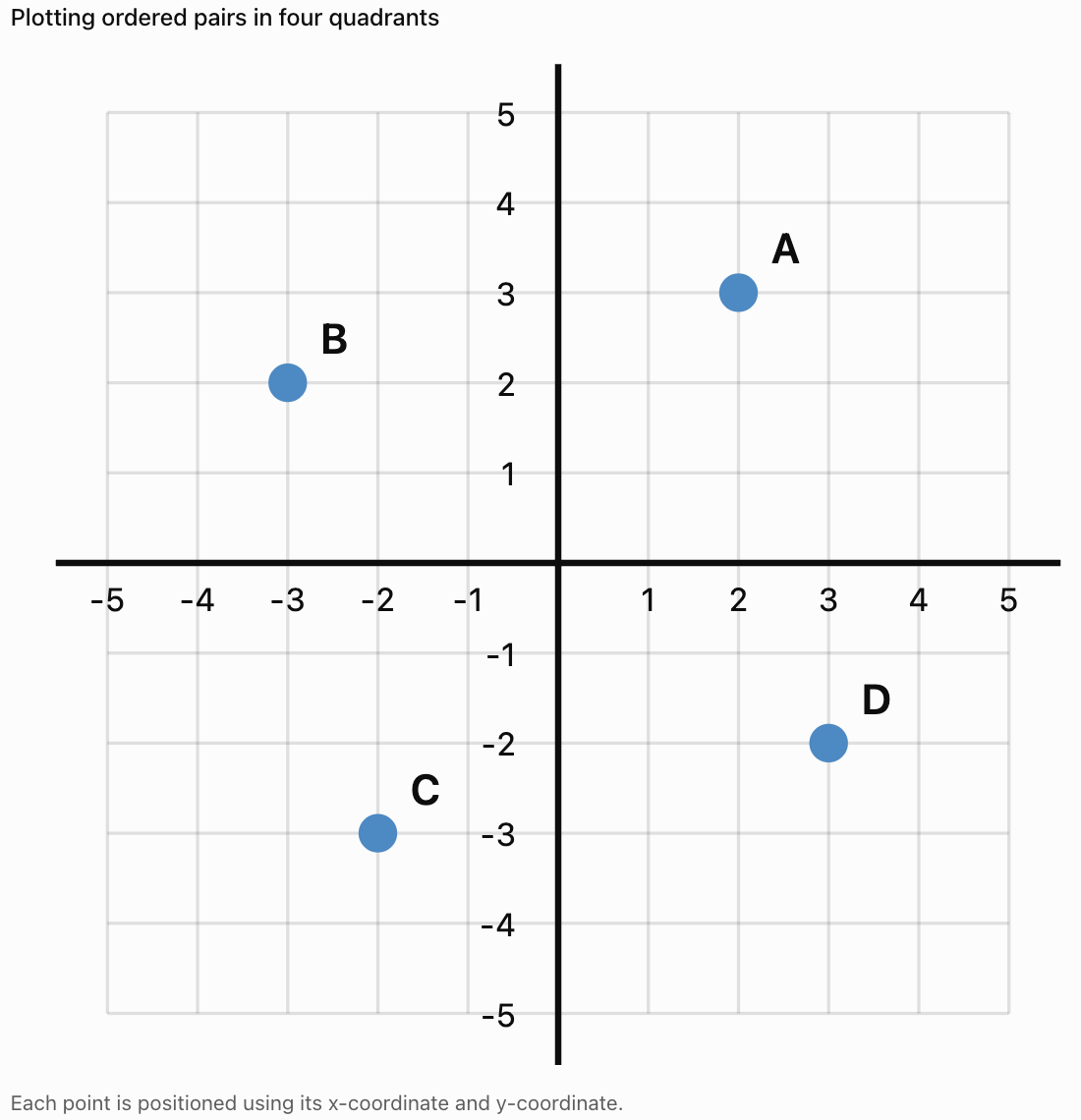
Plot the following points:
A = (2, 3)
B = (−3, 2)
C = (−2, −3)
D = (3, −2)
Important Observation
Ordered pairs provide exact locations on the coordinate plane.
What Is a Linear Relationship?
A linear relationship occurs when one variable changes at a constant rate relative to another.
Example
A student earns $5 for every hour worked.
|
Hours Worked (x) |
Earnings ($) |
|---|---|
|
0 |
0 |
|
1 |
5 |
|
2 |
10 |
|
3 |
15 |
|
4 |
20 |
Each additional hour increases earnings by $5.
This is a linear relationship.
Equation
y = 5x
where:
-
x = hours worked
-
y = total earnings
Important Observation
A constant rate of change produces a straight-line graph.
Creating Tables from Equations
A table of values can be created by substituting different x-values into an equation.
Worked Example
Consider:
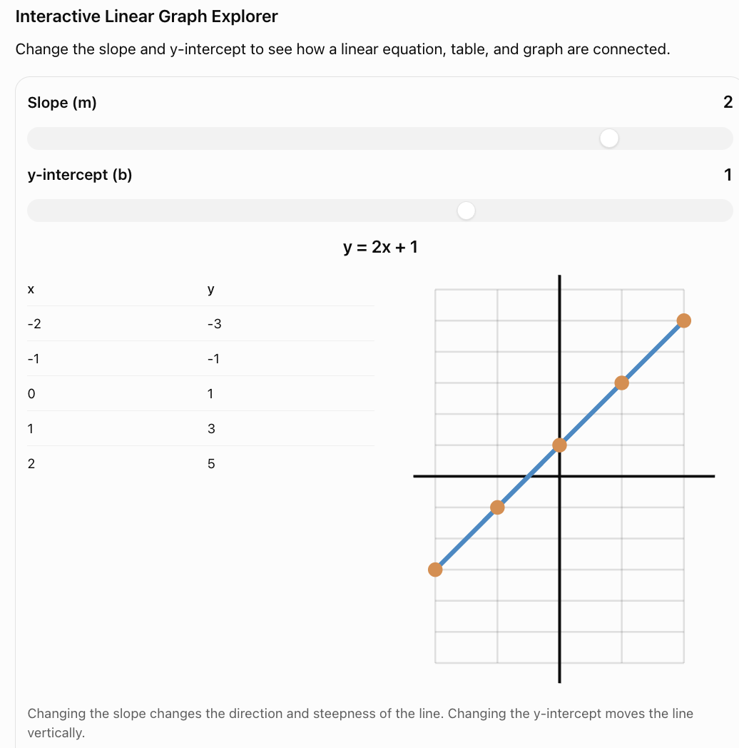
y = 2x + 1
Choose the x-values:
−2, −1, 0, 1, 2
Step 1: Substitute Each Value
When x = −2:
y = 2(−2) + 1 = −3
When x = −1:
y = 2(−1) + 1 = −1
When x = 0:
y = 2(0) + 1 = 1
When x = 1:
y = 2(1) + 1 = 3
When x = 2:
y = 2(2) + 1 = 5
Step 2: Organise the Values
|
x |
y |
|---|---|
|
−2 |
−3 |
|
−1 |
−1 |
|
0 |
1 |
|
1 |
3 |
|
2 |
5 |
Step 3: Write the Ordered Pairs
(−2, −3)
(−1, −1)
(0, 1)
(1, 3)
(2, 5)
These ordered pairs can now be plotted.
Creating a Graph from a Table
Worked Example
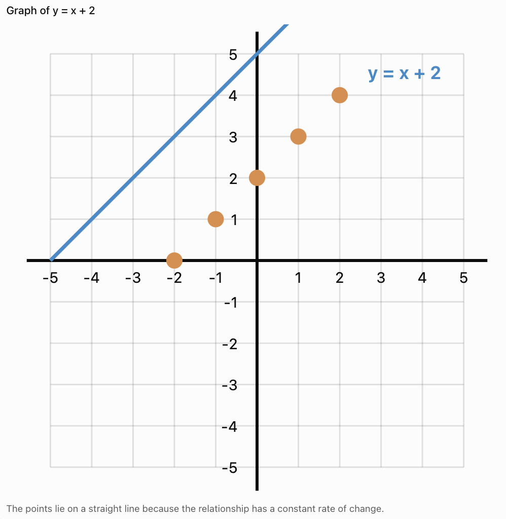
Graph the equation:
y = x + 2
Step 1: Create a Table
|
x |
y |
|---|---|
|
−2 |
0 |
|
−1 |
1 |
|
0 |
2 |
|
1 |
3 |
|
2 |
4 |
Step 2: Plot the Points
Step 3: Draw the Line
Use a ruler to draw a straight line through the points.
For a continuous linear relationship, extend the line appropriately.
Important Observation
The line represents all pairs of values satisfying the equation, not only the points originally listed in the table.
Recognising Linear Patterns in Tables
A linear relationship has a constant rate of change.
When x-values increase by equal amounts, the y-values change by equal amounts.
Example
|
x |
y |
|---|---|
|
1 |
4 |
|
2 |
7 |
|
3 |
10 |
|
4 |
13 |
|
5 |
16 |
The y-values increase by 3 each time x increases by 1.
Differences:
7 − 4 = 3
10 − 7 = 3
13 − 10 = 3
16 − 13 = 3
The rate of change is constant.
Equation
y = 3x + 1
Important Observation
A constant first difference indicates a linear relationship when the x-values are equally spaced.
Recognising Linear Patterns on Graphs
Linear relationships produce straight lines.
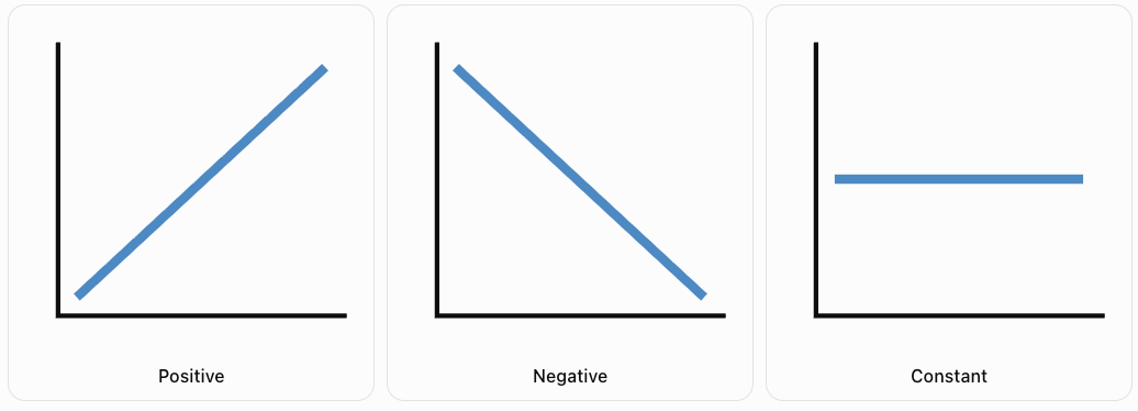
There are three common types of linear patterns.
Positive Linear Relationship
As x increases, y increases.
The line rises from left to right.
Negative Linear Relationship
As x increases, y decreases.
The line falls from left to right.
Constant Relationship
The y-value remains unchanged as x increases.
The line is horizontal.
Important Observation
The direction of a line reveals how the dependent variable changes as the independent variable increases.
Understanding Slope
The slope of a line measures its rate of change.
It describes how much y changes for a given change in x.
The slope is commonly represented by the letter m.
Formula
m = (y₂ − y₁)/(x₂ − x₁)
This can also be written as:
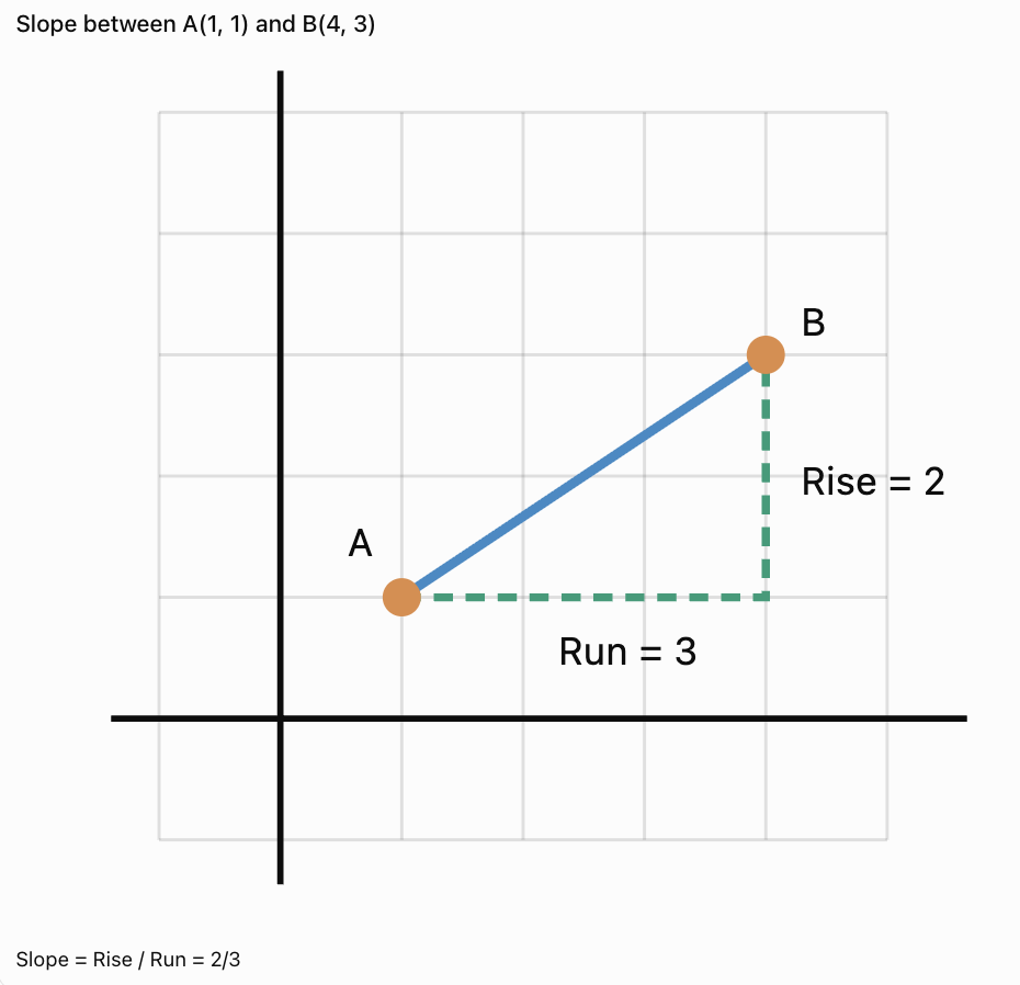
Slope = Rise / Run
where:
-
Rise = vertical change.
-
Run = horizontal change.
Worked Example
Find the slope of the line passing through:
A = (1, 3)
B = (4, 9)
Step 1: Calculate the Vertical Change
Rise = 9 − 3 = 6
Step 2: Calculate the Horizontal Change
Run = 4 − 1 = 3
Step 3: Divide
m = 6/3
m = 2
Interpretation
For every increase of 1 in x, y increases by 2.
Visualising Rise and Run
Important Observation
Slope can be positive, negative, zero, or undefined.
Positive, Negative, Zero, and Undefined Slope
Positive Slope
A line rises from left to right.
Example:
y = 2x + 1
Slope = 2
Negative Slope
A line falls from left to right.
Example:
y = −3x + 4
Slope = −3
Zero Slope
A horizontal line has slope zero.
Example:
y = 5
Slope = 0
Undefined Slope
A vertical line has an undefined slope because the horizontal change is zero.
Example:
x = 3
Important Observation
Vertical lines cannot be written in the form y = mx + b because their slope is undefined.
Slope-Intercept Form
Many linear equations can be written as:
y = mx + b
where:
-
m = slope.
-
b = y-intercept.
The y-intercept is the point where the line crosses the y-axis.
At the y-intercept:
x = 0
Example
Consider:
y = 3x + 2
Slope = 3
y-intercept = 2
The line crosses the y-axis at:
(0, 2)
Important Observation
The slope tells us how the line changes, while the y-intercept tells us where the line crosses the y-axis.
Graphing from Slope and y-Intercept
Worked Example
Graph:
y = 2x + 1
Step 1: Identify the y-Intercept
b = 1
Plot:
(0, 1)
Step 2: Identify the Slope
m = 2
This can be written:
2/1
Move:
-
1 unit right.
-
2 units up.
Step 3: Plot Another Point
Starting at (0, 1), moving right 1 and up 2 gives:
(1, 3)
Step 4: Draw the Line
Draw a straight line through the points.
Important Observation
A straight line is uniquely determined by two distinct points.
Additional points can be used to check accuracy.
Connecting Equations, Tables, and Graphs
A linear relationship can be represented in three main ways.
Equation
y = 2x + 3
Table
|
x |
y |
|---|---|
|
0 |
3 |
|
1 |
5 |
|
2 |
7 |
|
3 |
9 |
|
4 |
11 |
Graph
The points:
(0, 3), (1, 5), (2, 7), (3, 9), (4, 11)
lie on a straight line.
How the Representations Connect
-
The equation gives the mathematical rule.
-
The table shows selected input-output values.
-
The graph displays the relationship visually.
Important Observation
All three representations describe the same relationship.
Finding an Equation from a Table
Worked Example
Determine the equation represented by the table.
|
x |
y |
|---|---|
|
0 |
4 |
|
1 |
7 |
|
2 |
10 |
|
3 |
13 |
Step 1: Find the Rate of Change
The y-values increase by 3 for every increase of 1 in x.
Therefore:
m = 3
Step 2: Find the y-Intercept
When x = 0:
y = 4
Therefore:
b = 4
Step 3: Write the Equation
y = 3x + 4
Step 4: Verify
When x = 2:
y = 3(2) + 4
y = 10
This matches the table.
Finding an Equation from Two Points
Worked Example
Find the equation of the line passing through:
(1, 4) and (3, 10)
Step 1: Calculate the Slope
m = (10 − 4)/(3 − 1)
m = 6/2
m = 3
Step 2: Use y = mx + b
y = 3x + b
Step 3: Substitute a Known Point
Using (1, 4):
4 = 3(1) + b
4 = 3 + b
b = 1
Final Equation
y = 3x + 1
Important Observation
Two distinct points determine exactly one straight line.
Interpreting Points on a Graph
Every point on a graph represents a relationship between two quantities.
Example: Distance and Time
A cyclist travels at a constant speed of 4 m/s.
The equation is:
d = 4t
where:
-
d = distance in metres.
-
t = time in seconds.
Table
|
Time (s) |
Distance (m) |
|---|---|
|
0 |
0 |
|
1 |
4 |
|
2 |
8 |
|
3 |
12 |
|
4 |
16 |
Interpreting a Point
The point (3, 12) means:
After 3 seconds, the cyclist has travelled 12 metres.
Important Observation
A graph point should always be interpreted using the quantities and units represented by the axes.
Interpreting Lines in Real-World Situations
A line represents the overall relationship between two variables.
Example: Taxi Fare
A taxi company charges:
-
A starting fee of $4.
-
An additional $2 per kilometre.
The equation is:
C = 2d + 4
where:
-
C = total cost in dollars.
-
d = distance in kilometres.
Table
|
Distance (km) |
Cost ($) |
|---|---|
|
0 |
4 |
|
1 |
6 |
|
2 |
8 |
|
3 |
10 |
|
4 |
12 |
Interpretation
The slope is 2.
This means the fare increases by $2 for each additional kilometre.
The y-intercept is 4.
This represents the starting fee.
Important Observation
The slope and y-intercept often have meaningful interpretations in practical situations.
Comparing Two Linear Relationships
Graphs can be used to compare different relationships.
Worked Example
Two companies offer delivery services.
Company A:
C = 3d + 5
Company B:
C = 2d + 9
where C is cost in dollars and d is distance in kilometres.
Table
|
Distance (km) |
Company A ($) |
Company B ($) |
|---|---|---|
|
0 |
5 |
9 |
|
1 |
8 |
11 |
|
2 |
11 |
13 |
|
3 |
14 |
15 |
|
4 |
17 |
17 |
|
5 |
20 |
19 |
Interpretation
Company A has a lower starting fee but a higher cost per kilometre.
Company B has a higher starting fee but a lower cost per kilometre.
At 4 km, both companies charge $17.
Finding the Intersection
Set the equations equal:
3d + 5 = 2d + 9
d = 4
Substitute:
C = 3(4) + 5 = 17
Intersection = (4, 17)
Important Observation
The intersection of two lines represents a point where the two relationships have the same output value for the same input.
Linear Relationships in Science
Linear relationships are common in scientific investigations.
Example: Hooke's Law
For a spring obeying Hooke's law:
F = kx
where:
-
F = force.
-
k = spring constant.
-
x = extension.
If k remains constant, force is directly proportional to extension.

Example
Suppose k = 20 N/m.
|
Extension (m) |
Force (N) |
|---|---|
|
0.00 |
0 |
|
0.05 |
1 |
|
0.10 |
2 |
|
0.15 |
3 |
|
0.20 |
4 |
The graph is a straight line through the origin.
Important Observation
A straight-line graph can reveal a constant relationship between physical quantities.
Hooke's law applies only while the spring remains within its linear elastic range.
Linear Relationships in Everyday Life
Earnings
If a worker earns $12 per hour:
E = 12h
Savings
If a person begins with $50 and saves $10 each week:
S = 10w + 50
Distance
If a vehicle travels at a constant speed of 60 km/h:
d = 60t
Water Usage
If a tank contains 200 L and loses 5 L per minute:
V = 200 − 5t
Important Observation
The slope represents a rate of change, while the intercept often represents an initial value.
When Is a Relationship Not Linear?
Not every relationship produces a straight line.
Example
Consider:
y = x²
|
x |
y |
|---|---|
|
0 |
0 |
|
1 |
1 |
|
2 |
4 |
|
3 |
9 |
|
4 |
16 |
The y-values do not increase by a constant amount.
The graph is curved.
Comparison
|
Linear |
Nonlinear |
|---|---|
|
Constant rate of change |
Changing rate of change |
|
Straight-line graph |
Often curved graph |
|
Example: y = 3x + 2 |
Example: y = x² |
|
Constant slope |
Slope may change |
Important Observation
A straight-line pattern indicates a linear relationship.
A curved graph generally indicates a nonlinear relationship.
Interpolation and Extrapolation
Linear graphs can be used to estimate unknown values.
Interpolation
Interpolation means estimating values between known data points.
Example
A cyclist travels:
-
8 m after 2 seconds.
-
16 m after 4 seconds.
Assuming constant speed, the distance after 3 seconds is:
12 m
Extrapolation
Extrapolation means predicting values beyond the known data range.
Example
If the cyclist continues at the same speed, the predicted distance after 6 seconds is:
24 m
Important Observation
Extrapolation assumes the linear pattern continues.
This may not always be realistic.
Common Mistakes
Reversing ordered pairs
Coordinates must be written (x, y).
Plotting points inaccurately
Always check both coordinate values.
Using an inconsistent scale
Graph intervals must be evenly spaced.
Confusing slope and y-intercept
Slope describes rate of change. The y-intercept describes where the line crosses the y-axis.
Forgetting negative slopes
A negative slope means y decreases as x increases.
Assuming all lines pass through the origin
Only lines with y-intercept zero pass through the origin.
Connecting points incorrectly
Linear relationships should produce straight lines.
Assuming every relationship is linear
A constant rate of change is required.
Ignoring units
Real-world graphs must include appropriate units.
Extending graphs beyond meaningful values
For example, negative time or negative distance may not make sense in a particular situation.
Misinterpreting graph intersections
An intersection represents equal output values at the same input.
Key Terms
-
Linear Relationship: Relationship with a constant rate of change.
-
Coordinate Plane: Grid used to locate points.
-
x-Axis: Horizontal axis.
-
y-Axis: Vertical axis.
-
Origin: Point (0, 0).
-
Ordered Pair: Coordinates written (x, y).
-
x-Coordinate: Horizontal position of a point.
-
y-Coordinate: Vertical position of a point.
-
Table of Values: Organised list of related input and output values.
-
Independent Variable: Input quantity, usually represented by x.
-
Dependent Variable: Output quantity, usually represented by y.
-
Slope: Rate of change of a line.
-
Rise: Vertical change between two points.
-
Run: Horizontal change between two points.
-
Positive Slope: Line rises from left to right.
-
Negative Slope: Line falls from left to right.
-
Zero Slope: Slope of a horizontal line.
-
Undefined Slope: Slope of a vertical line.
-
y-Intercept: Point where a line crosses the y-axis.
-
x-Intercept: Point where a line crosses the x-axis.
-
Slope-Intercept Form: Equation written y = mx + b.
-
Rate of Change: Change in one quantity relative to another.
-
Linear Equation: Equation whose graph is a straight line.
-
Intersection: Point where two graphs meet.
-
Interpolation: Estimating values within known data.
-
Extrapolation: Predicting values beyond known data.
-
Nonlinear Relationship: Relationship without a constant rate of change.
Key Takeaways
-
Linear relationships have a constant rate of change.
-
Linear graphs are straight lines.
-
Ordered pairs represent points on a coordinate plane.
-
Tables can be used to generate graph points.
-
Equations can be used to create tables of values.
-
The slope measures the rate of change.
-
Positive slopes rise from left to right.
-
Negative slopes fall from left to right.
-
Horizontal lines have zero slope.
-
Vertical lines have undefined slope.
-
The y-intercept is where the line crosses the y-axis.
-
Linear equations can often be written as y = mx + b.
-
Equations, tables, and graphs represent the same relationships in different ways.
-
Graph points have meaningful interpretations in real-world situations.
-
Intersections represent equal values of two relationships.
-
Linear graphs can be used to estimate and predict values.
Check Your Understanding
Plotting Ordered Pairs
-
What is an ordered pair?
-
Which coordinate is plotted first?
-
Plot the point (3, 4).
-
Plot the point (−2, 5).
-
Explain why (2, 3) and (3, 2) represent different points.
Creating Graphs from Tables
-
Create a table for y = 2x when x = 0, 1, 2, 3, 4.
-
Create a table for y = x + 3 when x = −2, −1, 0, 1, 2.
-
Write the ordered pairs from Question 7.
-
Explain how a table can be used to create a graph.
-
What shape does the graph of a linear relationship form?
Identifying Linear Patterns
-
A table contains y-values 4, 7, 10, 13, 16 for x-values 0, 1, 2, 3, 4. Is the relationship linear?
-
What is the rate of change in Question 11?
-
A line rises from left to right. Is its slope positive or negative?
-
What is the slope of a horizontal line?
-
What is the slope of a vertical line?
Interpreting Linear Relationships
-
What does the slope represent?
-
What does the y-intercept represent?
-
A taxi fare is described by C = 3d + 5. What does the number 5 represent?
-
A cyclist travels according to d = 4t. What distance is travelled after 6 seconds?
-
Explain how equations, tables, and graphs are connected.
Answer Key
|
Question |
Answer |
|---|---|
|
1 |
Pair of coordinates written (x, y) |
|
2 |
x-coordinate |
|
3 |
3 right, 4 up |
|
4 |
2 left, 5 up |
|
5 |
The coordinates are reversed |
|
6 |
y = 0, 2, 4, 6, 8 |
|
7 |
y = 1, 2, 3, 4, 5 |
|
8 |
(−2, 1), (−1, 2), (0, 3), (1, 4), (2, 5) |
|
9 |
Plot the ordered pairs and draw the appropriate graph |
|
10 |
Straight line |
|
11 |
Yes |
|
12 |
3 |
|
13 |
Positive |
|
14 |
Zero |
|
15 |
Undefined |
|
16 |
Rate of change |
|
17 |
Value of y when x = 0 |
|
18 |
Starting fee of $5 |
|
19 |
24 metres |
|
20 |
They are different representations of the same relationship |
Extended Challenge
1. Find the slope of the line passing through (2, 5) and (6, 13).
2. Determine the equation of the line passing through (0, 4) and (3, 10).
3. Create a table for y = −2x + 5 when x = 0, 1, 2, 3, 4.
4. A table shows x-values 1, 2, 3, 4 and y-values 6, 10, 14, 18. Determine the equation.
5. Find the y-intercept of y = 5x − 7.
6. Find the x-intercept of y = 2x − 8.
7. Two companies charge C = 4d + 3 and C = 2d + 11. Determine the distance at which their charges are equal.
8. A water tank contains 150 L and loses 6 L per minute. Write an equation for the water remaining after t minutes.
9. A cyclist travels at 5 m/s. Create a table showing distance travelled at 0, 2, 4, 6, and 8 seconds.
10. Explain why the relationship y = x² is nonlinear.
Extended Challenge Answers
|
Question |
Answer |
|---|---|
|
1 |
m = 2 |
|
2 |
y = 2x + 4 |
|
3 |
y = 5, 3, 1, −1, −3 |
|
4 |
y = 4x + 2 |
|
5 |
(0, −7) |
|
6 |
(4, 0) |
|
7 |
4 distance units |
|
8 |
V = 150 − 6t, for 0 ≤ t ≤ 25 |
|
9 |
0, 10, 20, 30, 40 m |
|
10 |
Its rate of change is not constant |
Final Investigation: Comparing Transportation Costs
Two transportation companies offer different pricing plans.
Company A
-
Starting fee: $5
-
Cost per kilometre: $3
Company B
-
Starting fee: $11
-
Cost per kilometre: $2
Part A: Writing Equations
-
Write an equation for Company A.
-
Write an equation for Company B.
-
Identify the slope of each equation.
-
Identify the y-intercept of each equation.
-
Explain what the slope and y-intercept represent.
Part B: Creating Tables
-
Create a table for Company A using distances 0, 1, 2, 3, 4, 5, 6, 7, and 8 km.
-
Create a table for Company B using the same distances.
-
Compare the costs at 2 km.
-
Compare the costs at 5 km.
-
Determine the distance at which both companies charge the same amount.
Part C: Graphing
-
Draw a coordinate plane.
-
Label the x-axis Distance (km).
-
Label the y-axis Cost ($).
-
Plot the points for Company A.
-
Plot the points for Company B.
-
Draw both lines and label them.
Part D: Interpreting the Graph
-
Which company has the lower starting fee?
-
Which company has the lower cost per kilometre?
-
Which company is cheaper for shorter journeys?
-
Which company is cheaper for longer journeys?
-
Explain what the intersection of the two lines represents.
-
Recommend which company a customer should choose for a journey of 10 km.
Investigation Answer Check
Equations
Company A:
C = 3d + 5
Company B:
C = 2d + 11
Tables
|
Distance (km) |
Company A ($) |
Company B ($) |
|---|---|---|
|
0 |
5 |
11 |
|
1 |
8 |
13 |
|
2 |
11 |
15 |
|
3 |
14 |
17 |
|
4 |
17 |
19 |
|
5 |
20 |
21 |
|
6 |
23 |
23 |
|
7 |
26 |
25 |
|
8 |
29 |
27 |
Intersection
3d + 5 = 2d + 11
d = 6
Cost = 3(6) + 5
Cost = $23
Both companies charge $23 for a journey of 6 km.
Comparison
-
Company A is cheaper for journeys shorter than 6 km.
-
Both companies charge the same at 6 km.
-
Company B is cheaper for journeys longer than 6 km.
10 km Journey
Company A:
C = 3(10) + 5 = $35
Company B:
C = 2(10) + 11 = $31
Company B is cheaper by $4.
Final Reflection
Graphing linear relationships allows us to connect numerical information, algebraic equations, and visual representations.
By creating tables, plotting ordered pairs, identifying linear patterns, and interpreting slopes and intercepts, we can analyse relationships and make informed predictions.
These skills are essential for solving problems involving motion, cost, growth, measurement, and many other real-world situations.