Introduction to Graphing
| 站点: | Young Education |
| 课程: | Introduction to Algebra |
| 图书: | Introduction to Graphing |
| 打印: | Guest user |
| 日期: | 2026年11月9日 星期一 16:41 |
1. The Coordinate Plane
Learning outcomes
- I can identify the x-axis and y-axis.
- I can locate points using ordered pairs.
- I can plot points accurately on a coordinate plane.
- I can determine coordinates from a graph.
- I can describe the location of points using coordinates.
The Coordinate Plane
Introduction
A coordinate plane is a mathematical grid used to describe the exact position of points.
It is formed by two number lines that intersect at right angles:
-
The x-axis runs horizontally (left and right).
-
The y-axis runs vertically (up and down).
By using these two axes together, we can identify the location of any point on the plane using a pair of numbers.
Coordinate planes are important in mathematics because they allow us to:
-
Locate and plot points.
-
Describe positions accurately.
-
Draw geometric shapes.
-
Interpret graphs.
-
Represent mathematical relationships.
-
Solve problems involving maps, movement, and distance.
Coordinate systems are also used in navigation, computer graphics, engineering, physics, and geography.
Understanding the Coordinate Plane
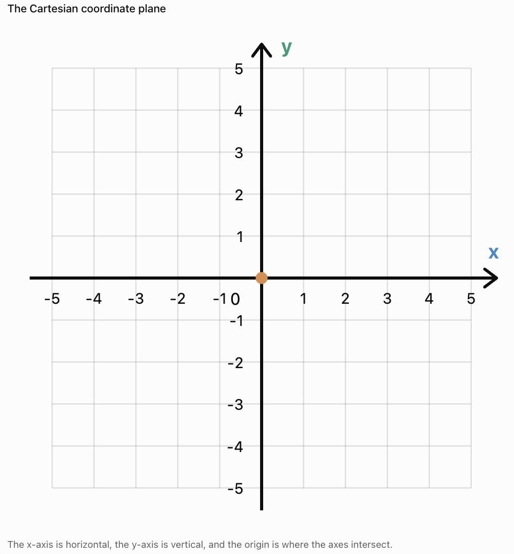
The coordinate plane is also called the Cartesian plane, named after the mathematician René Descartes.
The horizontal and vertical axes intersect at a point called the origin.
The origin has the coordinates:
(0, 0)
Important Features
-
Positive x-values are located to the right of the origin.
-
Negative x-values are located to the left of the origin.
-
Positive y-values are located above the origin.
-
Negative y-values are located below the origin.
Important Observation
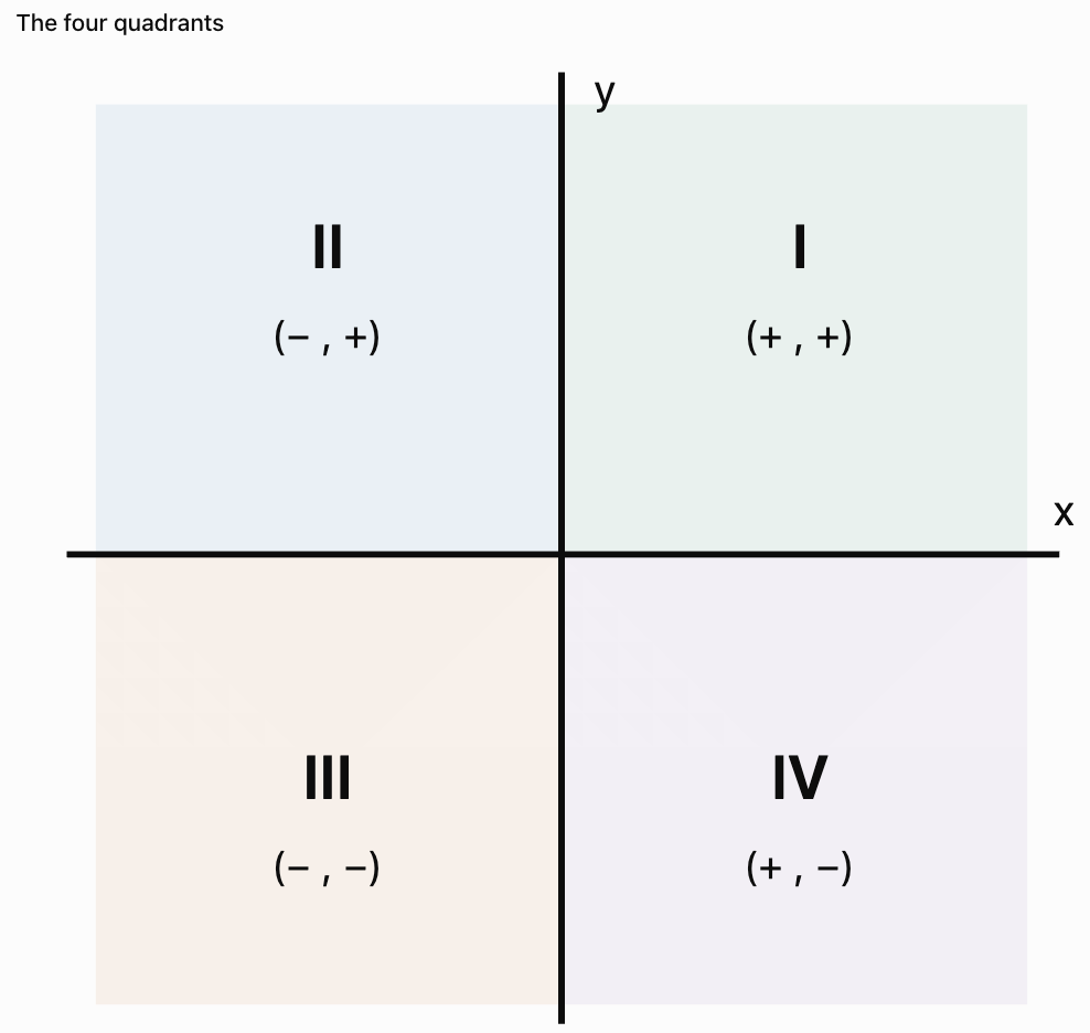
The axes divide the plane into four regions called quadrants.
The x-Axis
The x-axis is the horizontal number line on a coordinate plane.
It measures how far a point is positioned to the left or right of the origin.
Positive x-Coordinates
A positive x-coordinate indicates movement to the right.
For example:
x = 4
means four units to the right of the origin.
Negative x-Coordinates
A negative x-coordinate indicates movement to the left.
For example:
x = −3
means three units to the left of the origin.
Zero x-Coordinate
If x = 0, the point lies somewhere on the y-axis.
Important Observation
The x-coordinate describes horizontal position.
The y-Axis
The y-axis is the vertical number line on a coordinate plane.
It measures how far a point is positioned above or below the origin.
Positive y-Coordinates
A positive y-coordinate indicates movement upward.
For example:
y = 5
means five units above the origin.
Negative y-Coordinates
A negative y-coordinate indicates movement downward.
For example:
y = −2
means two units below the origin.
Zero y-Coordinate
If y = 0, the point lies somewhere on the x-axis.
Important Observation
The y-coordinate describes vertical position.
What Are Ordered Pairs?
A point on a coordinate plane is represented by an ordered pair.
An ordered pair contains two numbers written in parentheses:
(x, y)
The first number represents the x-coordinate.
The second number represents the y-coordinate.
Example
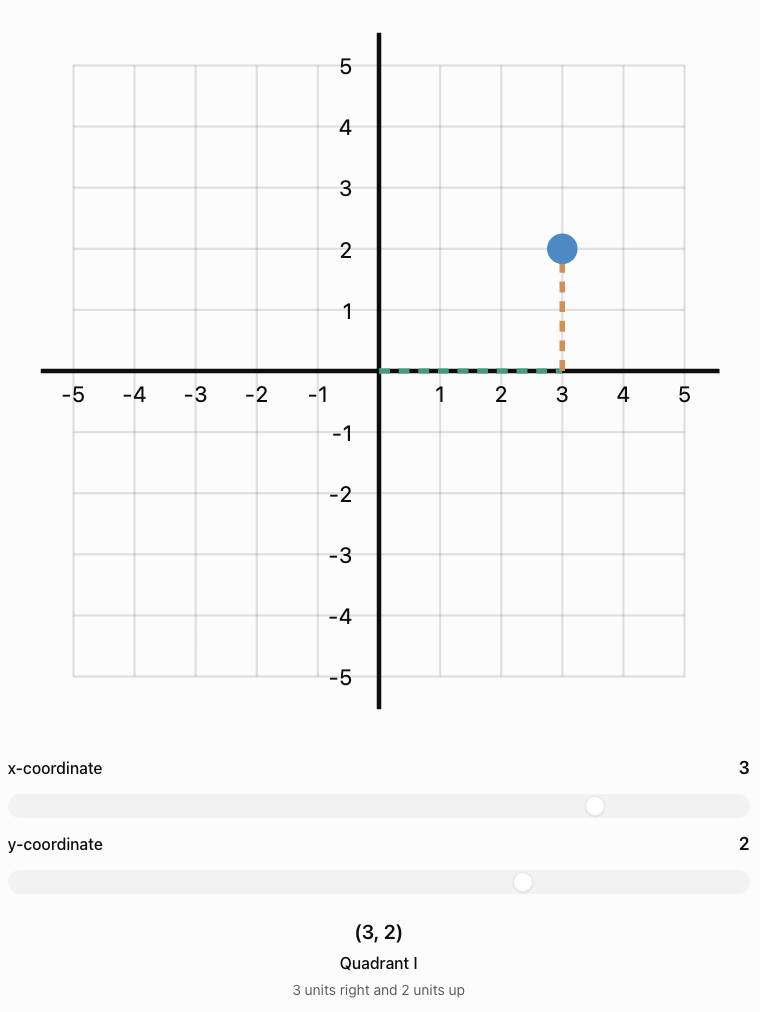
Consider the point:
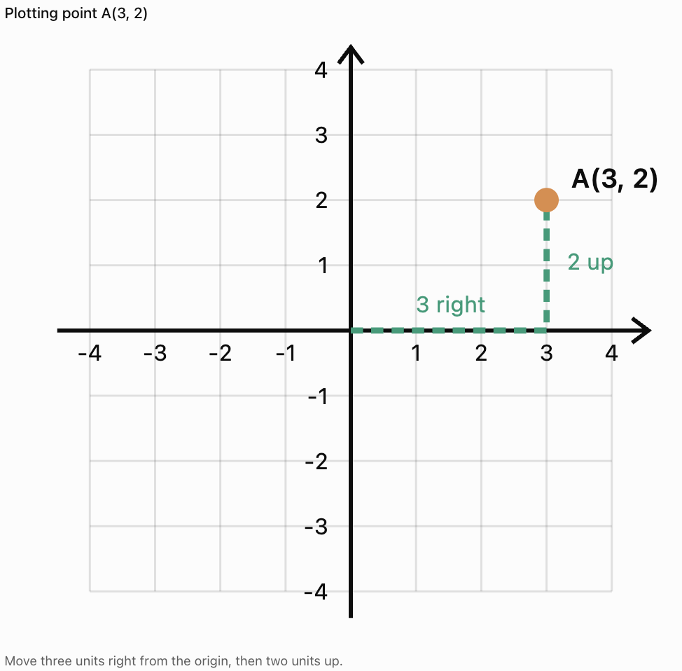
(3, 2)
This means:
-
Move 3 units to the right.
-
Move 2 units upward.
The point is located where these positions meet.
Remember
x first, y second.
A useful memory aid is:
Across first, then up or down.
Important Observation
The order of the numbers matters.
The points (3, 2) and (2, 3) are not the same location.
Plotting Points on the Coordinate Plane
To plot a point, begin at the origin.
Steps
-
Identify the x-coordinate.
-
Move horizontally according to the x-coordinate.
-
Identify the y-coordinate.
-
Move vertically according to the y-coordinate.
-
Mark the point.
-
Label the point if required.
Worked Example: Plotting (3, 2)
Important Observation
A point must be placed at the intersection of the correct vertical and horizontal grid lines.
Plotting Points with Negative Coordinates
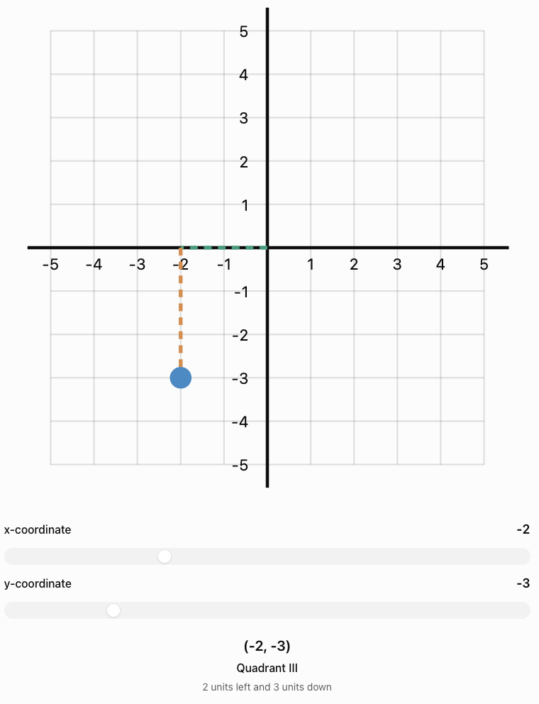
Negative coordinates describe positions to the left or below the origin.
Example: Plotting (−4, 3)
Start at (0, 0).
-
Move 4 units left.
-
Move 3 units up.
-
Mark the point.
Example: Plotting (2, −3)
Start at (0, 0).
-
Move 2 units right.
-
Move 3 units down.
-
Mark the point.
Example: Plotting (−2, −4)
Start at (0, 0).
-
Move 2 units left.
-
Move 4 units down.
-
Mark the point.
The Four Quadrants
The coordinate plane is divided into four quadrants.
The quadrants are numbered counterclockwise, beginning in the upper-right region.
Quadrant Rules
|
Quadrant |
x-coordinate |
y-coordinate |
Example |
|---|---|---|---|
|
I |
Positive |
Positive |
(3, 4) |
|
II |
Negative |
Positive |
(−3, 4) |
|
III |
Negative |
Negative |
(−3, −4) |
|
IV |
Positive |
Negative |
(3, −4) |
Important Observation
Points lying directly on an axis do not belong to any quadrant.
Identifying the Quadrant of a Point
Worked Example
Determine the quadrant containing each point.
A = (4, 5)
B = (−2, 6)
C = (−3, −4)
D = (5, −2)
Solutions
-
A has positive x and positive y, so it lies in Quadrant I.
-
B has negative x and positive y, so it lies in Quadrant II.
-
C has negative x and negative y, so it lies in Quadrant III.
-
D has positive x and negative y, so it lies in Quadrant IV.
Important Observation
You can identify a quadrant using only the signs of the coordinates.
Points on the Axes
Not every point lies inside a quadrant.
Some points lie directly on the x-axis or y-axis.
Points on the x-Axis
Every point on the x-axis has:
y = 0
Examples:
(3, 0)
(−5, 0)
(0, 0)
Points on the y-Axis
Every point on the y-axis has:
x = 0
Examples:
(0, 4)
(0, −2)
(0, 0)
The Origin
The origin is:
(0, 0)
It lies on both axes.
Important Observation
The origin is not part of any quadrant.
Reading Coordinates from a Graph
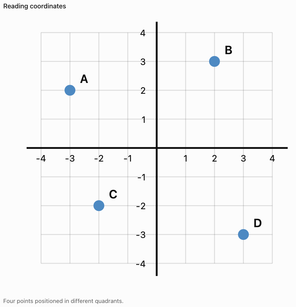
Sometimes a graph shows a point, and we must determine its coordinates.
Method
-
Locate the point.
-
Read its horizontal position on the x-axis.
-
Read its vertical position on the y-axis.
-
Write the coordinates in the form (x, y).
Example
Answers
-
A = (−3, 2)
-
B = (2, 3)
-
C = (−2, −2)
-
D = (3, −3)
Important Observation
Always read the x-coordinate before the y-coordinate.
Describing the Location of Points
Coordinates allow us to describe locations precisely.
Example
Consider the point:
P = (−5, 2)
We can describe its position as:
"Point P is five units left of the origin and two units above it."
Another example:
Q = (4, −3)
"Point Q is four units right of the origin and three units below it."
Important Observation
Coordinate descriptions should include both horizontal and vertical position.
Comparing the Locations of Points
Coordinates also allow us to compare points.
Example
A = (2, 4)
B = (5, 4)
Both points have the same y-coordinate.
Therefore, they lie on the same horizontal line.
Point B is three units to the right of point A.
Another Example
C = (−3, 2)
D = (−3, −4)
Both points have the same x-coordinate.
Therefore, they lie on the same vertical line.
Point D is six units below point C.
Important Observation
-
Equal x-coordinates indicate vertical alignment.
-
Equal y-coordinates indicate horizontal alignment.
Horizontal and Vertical Distance
Coordinates can be used to calculate distances between points lying on the same horizontal or vertical line.
Horizontal Distance
If two points have the same y-coordinate:
Horizontal distance = |x₂ − x₁|
Worked Example
A = (−2, 3)
B = (5, 3)
Distance = |5 − (−2)|
Distance = |7|
Distance = 7 units
Vertical Distance
If two points have the same x-coordinate:
Vertical distance = |y₂ − y₁|
Worked Example
C = (4, −3)
D = (4, 5)
Distance = |5 − (−3)|
Distance = 8 units
Important Observation
Distance is always non-negative.
Drawing Shapes on a Coordinate Plane
Coordinate planes can be used to create geometric shapes.
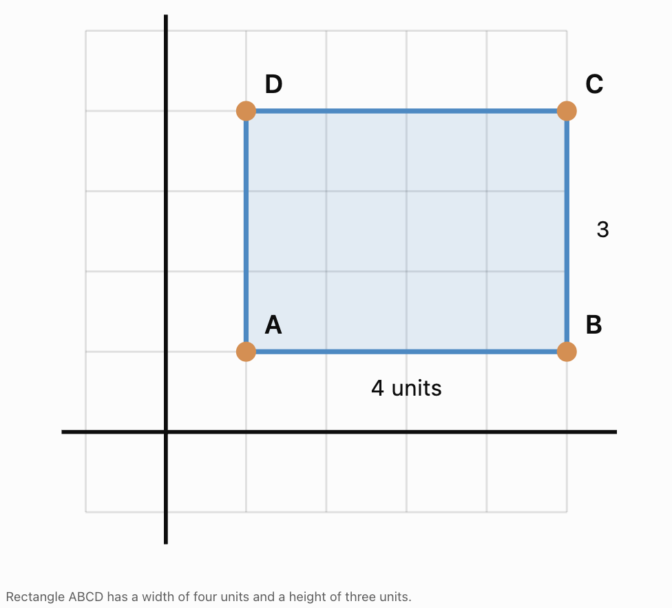
Example: Drawing a Rectangle
Plot the following points:
A = (1, 1)
B = (5, 1)
C = (5, 4)
D = (1, 4)
Connect the points in order:
A → B → C → D → A
Finding the Perimeter
Width = 5 − 1 = 4 units
Height = 4 − 1 = 3 units
Perimeter = 2(4 + 3)
Perimeter = 14 units
Finding the Area
Area = length × width
Area = 4 × 3
Area = 12 square units
Coordinate Planes in Maps
Coordinate systems are useful for locating objects on maps.

Example
A simplified map uses coordinates to identify locations.
-
School = (2, 3)
-
Library = (5, 3)
-
Park = (5, 6)
-
Sports Centre = (1, 6)
Questions
Which locations lie on the same horizontal line?
The school and library both have y = 3.
Which locations lie on the same vertical line?
The library and park both have x = 5.
Important Observation
Coordinate systems provide a precise way to describe locations without relying only on verbal directions.
Coordinate Planes in Computer Graphics
Computer graphics use coordinate systems to position objects on screens.

Examples include:
-
Video games.
-
Animation.
-
Graphic design.
-
Digital maps.
-
Computer-aided design.
Important Difference
In many computer screen coordinate systems, the origin is located in the upper-left corner.
The y-coordinate often increases downward rather than upward.
This is different from the usual mathematical coordinate plane.
Important Observation
Coordinate conventions must always be checked before interpreting positions.
Coordinate Planes in Physics
Coordinate systems are used to describe position and motion.

Example
A moving object begins at:
A = (0, 0)
It then moves to:
B = (4, 3)
Its horizontal displacement is:
Δx = 4 − 0 = 4 units
Its vertical displacement is:
Δy = 3 − 0 = 3 units
Important Observation
Coordinate systems allow scientists to describe movement in different directions.
Interactive Coordinate Practice
Use the sliders to move a point around the coordinate plane. Observe how its ordered pair and quadrant change.
Common Mistakes
Reversing the coordinates
The correct order is always (x, y).
Confusing the axes
The x-axis is horizontal; the y-axis is vertical.
Forgetting negative directions
Negative x-values move left; negative y-values move down.
Starting from the wrong location
Always begin plotting from the origin.
Counting grid lines incorrectly
Move the correct number of spaces or units, rather than counting the starting line as one unit.
Confusing quadrants
Quadrants are numbered counterclockwise, beginning in the upper-right region.
Placing points on the wrong axis
A point with y = 0 lies on the x-axis.
A point with x = 0 lies on the y-axis.
Assuming the origin belongs to a quadrant
The origin lies on both axes and belongs to no quadrant.
Ignoring the scale
Not all coordinate grids increase by one unit per square.
Confusing horizontal and vertical distance
Horizontal distance depends on x-coordinates; vertical distance depends on y-coordinates.
Key Terms
-
Coordinate Plane: Two-dimensional grid used to locate points.
-
Cartesian Plane: Another name for the coordinate plane.
-
x-Axis: Horizontal number line.
-
y-Axis: Vertical number line.
-
Origin: Intersection of the axes at (0, 0).
-
Ordered Pair: Two numbers representing a point's location, written (x, y).
-
x-Coordinate: First number in an ordered pair, indicating horizontal position.
-
y-Coordinate: Second number in an ordered pair, indicating vertical position.
-
Quadrant: One of the four regions formed by the axes.
-
Plot: Mark a point at its coordinates.
-
Point: Exact location on the coordinate plane.
-
Horizontal: Direction parallel to the x-axis.
-
Vertical: Direction parallel to the y-axis.
-
Positive Coordinate: Coordinate indicating rightward or upward position in the standard plane.
-
Negative Coordinate: Coordinate indicating leftward or downward position in the standard plane.
-
Coordinate Grid: Network of horizontal and vertical lines used to locate points.
-
Scale: Value represented by each interval on an axis.
-
Distance: Separation between two points.
-
Horizontal Distance: Difference between x-coordinates of horizontally aligned points.
-
Vertical Distance: Difference between y-coordinates of vertically aligned points.
-
Displacement: Change in position.
-
Quadrant I: Region with positive x and positive y.
-
Quadrant II: Region with negative x and positive y.
-
Quadrant III: Region with negative x and negative y.
-
Quadrant IV: Region with positive x and negative y.
Key Takeaways
-
A coordinate plane contains two perpendicular axes.
-
The x-axis is horizontal.
-
The y-axis is vertical.
-
The axes intersect at the origin (0, 0).
-
Points are represented using ordered pairs.
-
The x-coordinate is written first.
-
The y-coordinate is written second.
-
Positive x-values move right.
-
Negative x-values move left.
-
Positive y-values move up.
-
Negative y-values move down.
-
The coordinate plane has four quadrants.
-
Points on an axis do not belong to a quadrant.
-
Coordinates can be used to plot points and describe locations.
-
Equal x-coordinates indicate vertical alignment.
-
Equal y-coordinates indicate horizontal alignment.
-
Coordinate systems are useful in mathematics, science, navigation, and technology.
Check Your Understanding
Understanding the Coordinate Plane
-
What is the coordinate plane?
-
Which axis is horizontal?
-
Which axis is vertical?
-
What are the coordinates of the origin?
-
What is an ordered pair?
Plotting Points
-
Describe how to plot the point (3, 4).
-
Describe how to plot the point (−2, 5).
-
Describe how to plot the point (4, −3).
-
Describe how to plot the point (−3, −2).
-
Explain why (2, 5) and (5, 2) are different points.
Identifying Quadrants
-
Which quadrant contains (4, 6)?
-
Which quadrant contains (−3, 5)?
-
Which quadrant contains (−4, −2)?
-
Which quadrant contains (5, −3)?
-
Does the point (0, 4) belong to a quadrant?
Applying Coordinates
-
Two points are A = (2, 3) and B = (6, 3). Find the distance between them.
-
Two points are C = (−2, −3) and D = (−2, 4). Find the distance between them.
-
A point lies four units left and two units above the origin. What are its coordinates?
-
A point lies three units right and five units below the origin. What are its coordinates?
-
Explain how coordinates can be used to describe locations on a map.
Answer Key
|
Question |
Answer |
|---|---|
|
1 |
A two-dimensional grid formed by two perpendicular number lines |
|
2 |
x-axis |
|
3 |
y-axis |
|
4 |
(0, 0) |
|
5 |
A pair of numbers describing horizontal and vertical position |
|
6 |
Move 3 right and 4 up |
|
7 |
Move 2 left and 5 up |
|
8 |
Move 4 right and 3 down |
|
9 |
Move 3 left and 2 down |
|
10 |
The x- and y-coordinates are reversed |
|
11 |
Quadrant I |
|
12 |
Quadrant II |
|
13 |
Quadrant III |
|
14 |
Quadrant IV |
|
15 |
No; it lies on the y-axis |
|
16 |
4 units |
|
17 |
7 units |
|
18 |
(−4, 2) |
|
19 |
(3, −5) |
|
20 |
Each location is assigned a precise ordered pair |
Extended Challenge
1. Plot A = (−4, 3), B = (2, 3), C = (2, −2), and D = (−4, −2). Connect the points in order. What shape is formed?
2. Calculate the perimeter of the shape in Question 1.
3. Calculate the area of the shape in Question 1.
4. A point has a negative x-coordinate and positive y-coordinate. Which quadrant contains the point?
5. A point lies on the x-axis, seven units to the left of the origin. What are its coordinates?
6. A point lies on the y-axis, six units below the origin. What are its coordinates?
7. Two points are P = (−5, 4) and Q = (3, 4). Calculate the horizontal distance between them.
8. Two points are R = (2, −6) and S = (2, 5). Calculate the vertical distance between them.
9. A rectangle has vertices A = (1, 1), B = (6, 1), C = (6, 5), and D = (1, 5). Calculate its perimeter and area.
10. Explain why the points (−3, 4) and (3, −4) are not reflections across the x-axis or y-axis individually.
Extended Challenge Answers
|
Question |
Answer |
|---|---|
|
1 |
Rectangle |
|
2 |
22 units |
|
3 |
30 square units |
|
4 |
Quadrant II |
|
5 |
(−7, 0) |
|
6 |
(0, −6) |
|
7 |
8 units |
|
8 |
11 units |
|
9 |
Perimeter = 18 units; area = 20 square units |
|
10 |
Both coordinate signs change, corresponding to reflection through the origin |
Final Investigation: Designing a Coordinate Map
A school is creating a coordinate map of its campus.
The school places the origin at the centre of the campus.
The following locations are assigned coordinates:
|
Location |
Coordinates |
|---|---|
|
Main Building |
(0, 0) |
|
Library |
(4, 3) |
|
Science Building |
(−3, 4) |
|
Sports Centre |
(−4, −2) |
|
Cafeteria |
(3, −3) |
|
Bus Stop |
(0, −5) |
|
Garden |
(5, 0) |
Part A: Plotting the Map
-
Draw a coordinate plane from −6 to +6 on both axes.
-
Label the x-axis and y-axis.
-
Mark the origin.
-
Plot all seven locations.
-
Label each point clearly.
Part B: Describing Locations
-
Which location is at the origin?
-
Which location is in Quadrant I?
-
Which location is in Quadrant II?
-
Which location is in Quadrant III?
-
Which location is in Quadrant IV?
-
Which locations lie directly on an axis?
Part C: Comparing Positions
-
How far right of the origin is the library?
-
How far left of the origin is the Science Building?
-
How far below the origin is the Bus Stop?
-
Which location is farthest to the right?
-
Which location is farthest to the left?
Part D: Extending the Map
-
Add a new classroom at (−2, 2).
-
Add a new playground at (4, −4).
-
Describe the position of each new location relative to the origin.
-
Explain why coordinates are useful for creating accurate maps.
Investigation Answer Check
-
Main Building: Origin
-
Library: Quadrant I
-
Science Building: Quadrant II
-
Sports Centre: Quadrant III
-
Cafeteria: Quadrant IV
-
Bus Stop: Negative y-axis
-
Garden: Positive x-axis
-
Library: 4 units right of origin
-
Science Building: 3 units left of origin
-
Bus Stop: 5 units below origin
-
Farthest right: Garden
-
Farthest left: Sports Centre
-
New classroom: 2 units left and 2 units up
-
New playground: 4 units right and 4 units down
Final Reflection
The coordinate plane provides a simple but powerful method for describing locations.
By understanding the x-axis, y-axis, origin, ordered pairs, and quadrants, we can locate points precisely and interpret graphs accurately.
These skills form the foundation for graphing equations, studying geometric transformations, analysing motion, and solving many other mathematical problems.
2. Tables and Graphs
Learning outcomes
- I can organize data into tables.
- I can create tables from patterns and relationships.
- I can identify trends in data tables.
- I can use tables to generate graph points.
- I can interpret information from tables and graphs.
Tables and Graphs
Introduction
Tables and graphs are important tools for organising, representing, and interpreting information.
A table arranges data into rows and columns, making it easier to identify values, compare quantities, and recognise patterns.
A graph represents information visually, allowing us to observe trends, relationships, and changes.
Tables and graphs are used throughout mathematics, science, geography, economics, engineering, and everyday life.
For example:
-
Scientists record experimental measurements in tables.
-
Meteorologists use graphs to display temperature changes.
-
Businesses analyse sales and expenses.
-
Students use tables to recognise mathematical patterns.
-
Engineers graph relationships between physical quantities.
-
Schools use graphs to compare student performance.
Learning to organise and interpret data is an essential mathematical skill.


What Is a Data Table?
A data table is an organised arrangement of information using rows and columns.
Tables allow us to record values systematically and compare related quantities.
Example: Daily Temperature
|
Day |
Temperature (°C) |
|---|---|
|
Monday |
24 |
|
Tuesday |
26 |
|
Wednesday |
25 |
|
Thursday |
28 |
|
Friday |
30 |
The table shows temperatures recorded over five days.
Parts of a Table
A well-organised table usually includes:
-
Title: Describes the information.
-
Column headings: Identify the quantities being recorded.
-
Rows: Contain individual observations or records.
-
Units: Show how measurements are expressed.
-
Data values: Provide the actual information.
Important Observation
A good table should allow someone to understand the information without needing additional explanations.
Rows and Columns
A row runs horizontally across a table.
A column runs vertically down a table.
Example: Student Test Results
|
Student |
Mathematics |
Science |
|---|---|---|
|
A |
78 |
82 |
|
B |
85 |
88 |
|
C |
91 |
86 |
|
D |
74 |
80 |
Each row represents one student.
Each column represents a particular category of information.
Reading the Table
Student B scored:
-
85 in Mathematics.
-
88 in Science.
Student C received the highest Mathematics score.
Important Observation
Tables allow us to compare information both horizontally and vertically.
Organising Data Systematically
When collecting information, it is important to organise it consistently.
Example: Plant Growth Investigation
A student measures the height of a plant over five weeks.
|
Week |
Plant Height (cm) |
|---|---|
|
0 |
4 |
|
1 |
7 |
|
2 |
10 |
|
3 |
13 |
|
4 |
16 |
The data is arranged in chronological order.
This makes it easy to identify changes in plant height over time.

Important Observation
Organising data in a logical order makes patterns easier to recognise.
Independent and Dependent Variables
When tables represent mathematical or scientific relationships, they often contain two variables.
Independent Variable
The independent variable is the quantity that is deliberately changed or used as the input.
It is commonly represented by x.
Dependent Variable
The dependent variable is the quantity that changes in response to the independent variable.
It is commonly represented by y.
Example
A student investigates how distance travelled changes with time.
|
Time (s) |
Distance (m) |
|---|---|
|
0 |
0 |
|
1 |
3 |
|
2 |
6 |
|
3 |
9 |
|
4 |
12 |
Independent variable: Time
Dependent variable: Distance
Important Observation
The independent variable is usually placed in the first column of a table and on the horizontal axis of a graph.
The dependent variable is usually placed in the second column and on the vertical axis.
Creating Tables from Patterns
Tables can be constructed using mathematical rules.
Example: Adding Three
Consider the pattern:
3, 6, 9, 12, 15, ...
Each term increases by 3.
We can organise the pattern in a table.
|
Term Number |
Value |
|---|---|
|
1 |
3 |
|
2 |
6 |
|
3 |
9 |
|
4 |
12 |
|
5 |
15 |
The rule is:
Value = 3n
Finding the Next Value
For n = 6:
Value = 3 × 6
Value = 18
Important Observation
Tables help us connect number patterns to mathematical rules.
Creating Tables from Equations
An equation can be used to generate a table of values.
Worked Example
Consider:
y = 2x + 1
Choose several x-values:
−2, −1, 0, 1, 2
Substitute each value into the equation.
Calculations
When x = −2:
y = 2(−2) + 1 = −3
When x = −1:
y = 2(−1) + 1 = −1
When x = 0:
y = 2(0) + 1 = 1
When x = 1:
y = 2(1) + 1 = 3
When x = 2:
y = 2(2) + 1 = 5
Table of Values
|
x |
y |
|---|---|
|
−2 |
−3 |
|
−1 |
−1 |
|
0 |
1 |
|
1 |
3 |
|
2 |
5 |
Important Observation
Each row represents one pair of related values.
Converting Tables into Ordered Pairs
A table of x-values and y-values can be converted into ordered pairs.
An ordered pair is written:
(x, y)
The x-value is written first.
The y-value is written second.
Example
Using the table for y = 2x + 1:
|
x |
y |
Ordered Pair |
|---|---|---|
|
−2 |
−3 |
(−2, −3) |
|
−1 |
−1 |
(−1, −1) |
|
0 |
1 |
(0, 1) |
|
1 |
3 |
(1, 3) |
|
2 |
5 |
(2, 5) |
These ordered pairs can be plotted on a coordinate plane.
Important Observation
Tables provide a systematic way to generate points for graphs.
Plotting Points from a Table
A graph can be created by plotting the ordered pairs from a table.
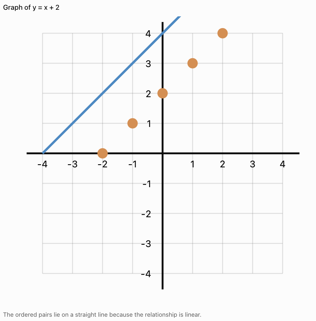
Worked Example
Graph the relationship:
y = x + 2
Step 1: Create a Table
|
x |
y |
|---|---|
|
−2 |
0 |
|
−1 |
1 |
|
0 |
2 |
|
1 |
3 |
|
2 |
4 |
Step 2: Write the Ordered Pairs
(−2, 0)
(−1, 1)
(0, 2)
(1, 3)
(2, 4)
Step 3: Plot the Points
Step 4: Interpret the Graph
As x increases by 1, y also increases by 1.
The graph is a straight line.
Important Observation
A table and a graph are two different representations of the same mathematical relationship.
Recognising Trends in Tables
A trend is a general pattern or direction in data.
Common trends include:
-
Increasing
-
Decreasing
-
Constant
-
Fluctuating
Increasing Trend
|
Time (min) |
Distance (m) |
|---|---|
|
0 |
0 |
|
1 |
5 |
|
2 |
10 |
|
3 |
15 |
Distance increases as time increases.
Decreasing Trend
|
Time (min) |
Water Remaining (L) |
|---|---|
|
0 |
20 |
|
1 |
17 |
|
2 |
14 |
|
3 |
11 |
The amount of water decreases over time.
Constant Trend
|
Time (min) |
Temperature (°C) |
|---|---|
|
0 |
25 |
|
1 |
25 |
|
2 |
25 |
|
3 |
25 |
The temperature remains unchanged.
Fluctuating Trend
|
Day |
Temperature (°C) |
|---|---|
|
Monday |
24 |
|
Tuesday |
27 |
|
Wednesday |
25 |
|
Thursday |
29 |
|
Friday |
26 |
The temperature rises and falls.
Important Observation
Identifying trends helps us describe how quantities change and make reasonable predictions.
Identifying Constant Differences
A table may show a pattern where the dependent variable changes by the same amount for every equal increase in the independent variable.
Example
|
x |
y |
|---|---|
|
1 |
4 |
|
2 |
7 |
|
3 |
10 |
|
4 |
13 |
|
5 |
16 |
The y-values increase by 3 each time x increases by 1.
Differences:
7 − 4 = 3
10 − 7 = 3
13 − 10 = 3
16 − 13 = 3
This is a linear relationship.
The rule is:
y = 3x + 1
Important Observation
A constant rate of change produces a straight-line graph.
Identifying Nonlinear Patterns
Not all relationships have constant differences.
Example
Consider:
y = x²
|
x |
y |
|---|---|
|
0 |
0 |
|
1 |
1 |
|
2 |
4 |
|
3 |
9 |
|
4 |
16 |
First differences:
1, 3, 5, 7
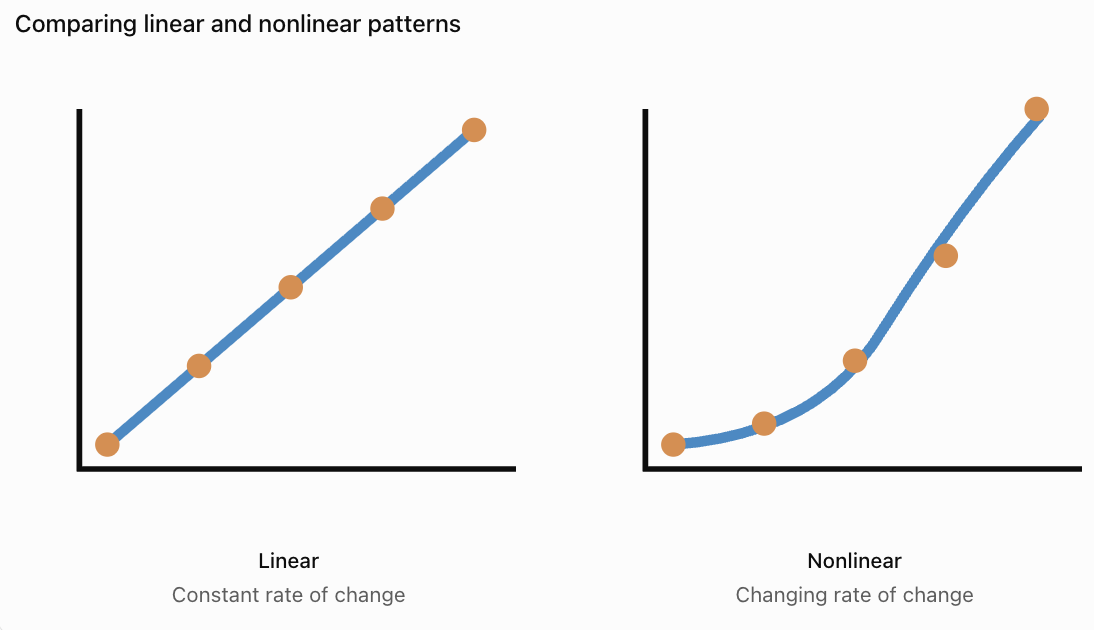
The differences are not constant.
However, the second differences are constant:
2, 2, 2
This is characteristic of a quadratic relationship when x-values are equally spaced.
Important Observation
Nonlinear relationships often produce curved graphs, although some nonlinear data may also produce other shapes.
Choosing the Correct Type of Graph
Different graphs are useful for different kinds of data.
Line Graphs
Line graphs are useful for showing changes in continuous quantities, especially over time.
Examples:
-
Temperature over time.
-
Distance travelled.
-
Population growth.
-
Water level changes.

Bar Graphs
Bar graphs are useful for comparing separate categories.
Examples:
-
Favourite school subjects.
-
Number of students in clubs.
-
Sales of different products.
-
Types of transportation used.

Scatter Plots
Scatter plots are useful for examining relationships between two numerical variables.
Examples:
-
Height and mass.
-
Study time and test scores.
-
Temperature and reaction rate.
-
Age and reaction time.

Important Observation
The best graph depends on the type of data and the relationship being investigated.
Creating a Line Graph from a Table
Worked Example: Plant Growth
A plant grows over five weeks.
|
Week |
Height (cm) |
|---|---|
|
0 |
4 |
|
1 |
7 |
|
2 |
10 |
|
3 |
13 |
|
4 |
16 |
Step 1: Identify the Variables
Independent variable: Week
Dependent variable: Plant height
Step 2: Label the Axes
x-axis: Week
y-axis: Height (cm)
Step 3: Choose a Scale
The x-axis should include weeks 0–4.
The y-axis should include heights from 0 to at least 16 cm.
Step 4: Plot the Points
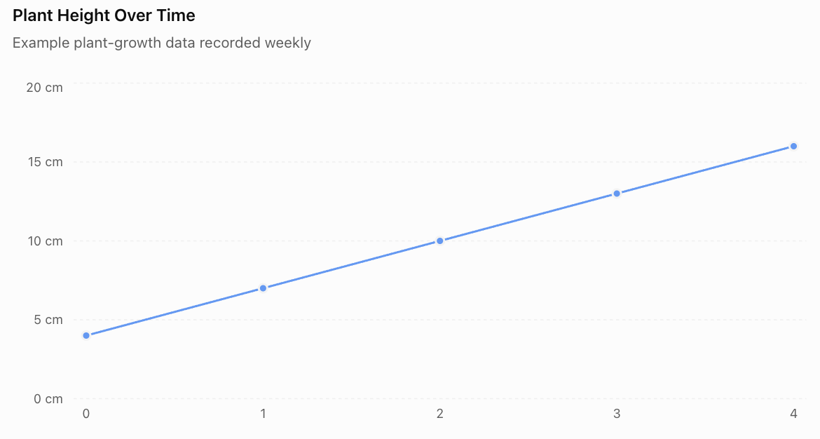
(0, 4)
(1, 7)
(2, 10)
(3, 13)
(4, 16)
Step 5: Connect the Points
Because the data describes a quantity changing over time, a line graph can be appropriate.
Step 6: Interpret the Graph
The plant grows by 3 cm each week.
The relationship is linear over the measured period.
Important Observation
The graph allows us to recognise the growth pattern more quickly than the table alone.
Interpreting Information from Graphs
Graphs provide information about quantities and their relationships.
When interpreting a graph, consider:
-
What does the title describe?
-
What does each axis represent?
-
What units are used?
-
What is the scale?
-
Does the graph increase, decrease, or remain constant?
-
Are there unusual values?
-
What conclusions can be drawn?
Example
A graph shows the temperature of water increasing from 20°C to 80°C over six minutes.
We can conclude that:
-
The water temperature increased.
-
The total increase was 60°C.
-
The average rate of temperature increase was 10°C per minute.
Calculation
Average rate = Change in temperature / Change in time
Average rate = (80 − 20)/6
Average rate = 10°C/min
Important Observation
Graphs allow us to calculate changes and rates of change.
Reading Values Between Data Points
Sometimes we need to estimate values that were not recorded directly.
This is called interpolation.
Example
A table shows:
|
Time (min) |
Temperature (°C) |
|---|---|
|
0 |
20 |
|
2 |
30 |
|
4 |
40 |
|
6 |
50 |
If the temperature changes steadily, we can estimate the temperature at 3 minutes.
Between 2 and 4 minutes, the temperature increases from 30°C to 40°C.
At 3 minutes, the estimated temperature is:
35°C
Important Observation
Interpolation estimates values within the range of observed data.
It is generally more reliable when the relationship is regular and the data is consistent.
Predicting Values Beyond the Data
Estimating values outside the recorded range is called extrapolation.
Example
A plant grows at a steady rate of 3 cm per week.
Its height at week 4 is 16 cm.
Predict its height at week 6.
Two additional weeks of growth:
2 × 3 = 6 cm
Predicted height:
16 + 6 = 22 cm
Important Observation
Extrapolation assumes the observed pattern continues.
This assumption may not be valid over long periods.
For example, plants do not grow at a constant rate forever.
Comparing Tables and Graphs
Tables and graphs have different strengths.
|
Tables |
Graphs |
|---|---|
|
Show exact numerical values |
Show visual patterns |
|
Organise detailed information |
Make trends easier to recognise |
|
Useful for calculations |
Useful for comparisons |
|
Allow precise data lookup |
Show relationships clearly |
|
Can contain many variables |
Often focus on selected relationships |
Important Observation
Tables and graphs complement each other.
A table provides detailed numerical information, while a graph makes patterns easier to see.
Tables and Graphs in Science
Scientists frequently collect data in tables and represent results using graphs.
Example: Heating Water
A student heats water and records its temperature.
|
Time (min) |
Temperature (°C) |
|---|---|
|
0 |
22 |
|
1 |
31 |
|
2 |
40 |
|
3 |
49 |
|
4 |
58 |
The table shows a constant increase of 9°C per minute.
A graph would show an upward-sloping straight line for these measurements.

Important Observation
Tables and graphs allow scientists to identify relationships between experimental variables.
Tables and Graphs in Everyday Life
Tables and graphs are also useful outside mathematics and science.
Examples
Personal Finance
A table can record monthly spending.
A graph can show changes in expenses over time.
Sports
A table can record scores.
A graph can show performance trends.
Weather
A table can record daily temperatures.
A graph can show changes throughout the week.
Education
A table can record test scores.
A graph can show improvement over time.
Transportation
A table can record journey times.
A graph can compare travel conditions.
Important Observation
Understanding tables and graphs helps us make informed decisions using evidence.
Interactive Table and Graph Explorer
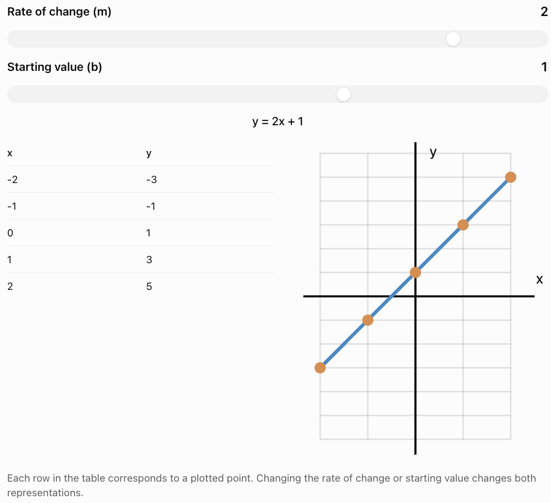
Change the values in a linear relationship and observe how the table and graph change.
Common Mistakes
Forgetting table headings
Every column should clearly identify the information it contains.
Leaving out units
Measurements should include appropriate units.
Mixing up independent and dependent variables
The independent variable is usually placed in the first column and on the x-axis.
Reversing ordered pairs
Ordered pairs are written (x, y), not (y, x).
Using an inappropriate graph type
Bar graphs compare categories, while line graphs are often used for continuous changes.
Choosing an inconsistent scale
Axis intervals should increase consistently unless a clearly labelled scale break is used.
Plotting points inaccurately
Points should be placed at the correct coordinate locations.
Connecting unrelated categories with a line
Connecting categories can incorrectly suggest continuous values between them.
Assuming every pattern is linear
Some relationships are curved or irregular.
Making unsupported predictions
Extrapolation may not be reliable if the pattern changes.
Ignoring unusual data
Unexpected values may indicate errors or meaningful changes in the relationship.
Key Terms
-
Data: Information collected through observations, measurements, or calculations.
-
Data Table: Organised arrangement of information using rows and columns.
-
Row: Horizontal arrangement of information in a table.
-
Column: Vertical arrangement of information in a table.
-
Heading: Label describing the information in a row or column.
-
Variable: Quantity that can change.
-
Independent Variable: Input quantity or variable deliberately changed.
-
Dependent Variable: Output quantity that depends on another variable.
-
Ordered Pair: Pair of coordinates written (x, y).
-
Coordinate Plane: Grid used to locate points.
-
Graph: Visual representation of data or mathematical relationships.
-
Line Graph: Graph showing how a quantity changes, often over time.
-
Bar Graph: Graph comparing categories using rectangular bars.
-
Scatter Plot: Graph showing relationships between paired numerical values.
-
Trend: General pattern or direction in data.
-
Increasing Trend: Pattern in which values generally rise.
-
Decreasing Trend: Pattern in which values generally fall.
-
Constant Trend: Pattern in which values remain unchanged.
-
Fluctuating Trend: Pattern in which values rise and fall.
-
Linear Relationship: Relationship with a constant rate of change.
-
Nonlinear Relationship: Relationship without a constant rate of change.
-
Rate of Change: Amount one quantity changes relative to another.
-
Scale: Numerical intervals used on a graph axis.
-
Interpolation: Estimating values within the observed data range.
-
Extrapolation: Estimating values outside the observed data range.
-
Pattern: Regularity or relationship in a set of values.
-
Prediction: Estimate based on observed information or a mathematical model.
Key Takeaways
-
Tables organise data into rows and columns.
-
Tables should include clear headings and appropriate units.
-
Independent variables are commonly placed in the first column.
-
Dependent variables are commonly placed in the second column.
-
Tables can be created from patterns and equations.
-
Each row of an x-y table can be written as an ordered pair.
-
Ordered pairs can be plotted on a coordinate plane.
-
Graphs make trends and relationships easier to recognise.
-
Linear relationships have constant rates of change.
-
Nonlinear relationships have changing rates of change.
-
Line graphs are useful for showing continuous changes.
-
Bar graphs are useful for comparing categories.
-
Scatter plots help identify relationships between numerical variables.
-
Tables provide exact values, while graphs show visual patterns.
-
Interpolation estimates values within a data range.
-
Extrapolation predicts values beyond the data range.
-
Tables and graphs are important tools in mathematics, science, and everyday life.
Check Your Understanding
Understanding Tables
-
What is a data table?
-
What is the difference between a row and a column?
-
Why should tables include headings?
-
Why are units important in data tables?
-
Explain the difference between an independent and dependent variable.
Creating Tables
-
Create a table for the pattern 2, 4, 6, 8, 10.
-
Create a table of values for y = 3x when x = 0, 1, 2, 3, 4.
-
Create a table for y = x + 4 when x = −2, −1, 0, 1, 2.
-
Convert the table from Question 8 into ordered pairs.
-
Explain how a table can be used to generate points for a graph.
Identifying Trends
-
A table shows values 5, 10, 15, 20, 25. Describe the trend.
-
A table shows values 30, 25, 20, 15, 10. Describe the trend.
-
A table shows values 12, 12, 12, 12. Describe the trend.
-
A table shows values 4, 7, 5, 9, 6. Describe the trend.
-
Explain how you can recognise a linear relationship from a table with equally spaced x-values.
Interpreting Graphs
-
What type of graph is useful for showing temperature changes over time?
-
What type of graph is useful for comparing favourite school subjects?
-
A graph shows distance increasing from 0 m to 100 m in 20 seconds. Calculate the average speed.
-
Explain the difference between interpolation and extrapolation.
-
Describe one advantage of a graph compared with a table.
Answer Key
|
Question |
Answer |
|---|---|
|
1 |
Organised arrangement of information using rows and columns |
|
2 |
Rows are horizontal; columns are vertical |
|
3 |
To identify the information being recorded |
|
4 |
To show how measurements are expressed |
|
5 |
Independent variable is the input; dependent variable responds to it |
|
6 |
Term numbers 1–5 paired with values 2, 4, 6, 8, 10 |
|
7 |
0, 3, 6, 9, 12 |
|
8 |
2, 3, 4, 5, 6 |
|
9 |
(−2, 2), (−1, 3), (0, 4), (1, 5), (2, 6) |
|
10 |
Each row provides an ordered pair (x, y) |
|
11 |
Increasing by 5 |
|
12 |
Decreasing by 5 |
|
13 |
Constant |
|
14 |
Fluctuating |
|
15 |
Equal changes in x produce equal changes in y |
|
16 |
Line graph |
|
17 |
Bar graph |
|
18 |
5 m/s |
|
19 |
Interpolation estimates within the data range; extrapolation estimates beyond it |
|
20 |
Graphs make trends and relationships easier to see |
Extended Challenge
1. Complete the table for y = 2x + 3 when x = −3, −2, −1, 0, 1, 2, 3.
2. A table contains the values x = 1, 2, 3, 4 and y = 5, 8, 11, 14. Determine the equation relating x and y.
3. A plant grows from 6 cm to 21 cm over five weeks. Calculate its average growth rate.
4. A car travels at a constant speed of 12 m/s. Create a table showing the distance travelled at 0, 1, 2, 3, 4, and 5 seconds.
5. A table shows x-values 0, 1, 2, 3, 4 and y-values 1, 4, 9, 16, 25. Determine a rule for the relationship.
6. A student records temperatures of 18°C, 22°C, 26°C, 30°C, and 34°C at equal time intervals. Describe the trend and calculate the increase between measurements.
7. Explain why a bar graph is more appropriate than a line graph for comparing the number of students in different clubs.
8. A table shows a constant increase of 7 units in y for every increase of 2 units in x. Determine the rate of change.
9. A graph shows that a water tank contains 120 L at 0 minutes and 60 L at 10 minutes. Calculate the average rate of change.
10. Explain why extrapolating a plant's growth rate over several years may be unreliable.
Extended Challenge Answers
|
Question |
Answer |
|---|---|
|
1 |
y = −3, −1, 1, 3, 5, 7, 9 |
|
2 |
y = 3x + 2 |
|
3 |
3 cm/week |
|
4 |
Distances: 0, 12, 24, 36, 48, 60 m |
|
5 |
y = (x + 1)² |
|
6 |
Increasing; 4°C per interval |
|
7 |
Clubs are separate categories rather than continuous values |
|
8 |
7/2 = 3.5 |
|
9 |
−6 L/min |
|
10 |
Growth rates change as plants mature and environmental conditions vary |
Final Investigation: Investigating a Mathematical Relationship
A student is investigating the relationship between time and distance travelled by a toy car moving at a constant speed.
The student records the following data:
|
Time (s) |
Distance (cm) |
|---|---|
|
0 |
0 |
|
1 |
15 |
|
2 |
30 |
|
3 |
45 |
|
4 |
60 |
|
5 |
75 |
Part A: Organising the Data
-
Identify the independent variable.
-
Identify the dependent variable.
-
Explain why the table is organised in this order.
-
Determine the increase in distance for each one-second interval.
-
Describe the trend shown in the table.
Part B: Creating a Graph
-
Draw a coordinate plane.
-
Label the x-axis as Time (s).
-
Label the y-axis as Distance (cm).
-
Choose appropriate scales.
-
Plot all six ordered pairs.
-
Connect the points appropriately.
-
Describe the shape of the graph.
Part C: Analysing the Relationship
-
Calculate the average speed of the toy car.
-
Write an equation relating distance and time.
-
Use the equation to predict the distance travelled after 7 seconds.
-
Estimate the distance travelled after 2.5 seconds.
-
Explain why the graph passes through the origin.
Part D: Evaluating the Data
-
Explain why a line graph is appropriate.
-
Describe one possible source of experimental error.
-
Explain how the student could improve the reliability of the investigation.
Investigation Answer Check
Variables
-
Independent variable: Time
-
Dependent variable: Distance
Trend
Distance increases by 15 cm each second.
Graph
The points form a straight line passing through the origin.
Average Speed
Speed = Distance / Time
Speed = 75/5
Speed = 15 cm/s
Equation
d = 15t
where d is distance in centimetres and t is time in seconds.
Prediction at 7 Seconds
d = 15 × 7
d = 105 cm
Interpolation at 2.5 Seconds
d = 15 × 2.5
d = 37.5 cm
Reliability
Repeating the investigation, using consistent measuring techniques, and averaging repeated measurements can improve reliability.
Final Reflection
Tables and graphs are essential tools for organising and interpreting information.
Tables allow us to record exact values and identify numerical patterns. Graphs make relationships and trends easier to recognise.
By learning to create tables, generate ordered pairs, plot graphs, and interpret data, we develop important mathematical skills that can be applied throughout science, technology, engineering, and everyday life.
3. Graphing Linear Relationships
Learning outcomes
- I can plot ordered pairs on a graph.
- I can create graphs from tables of values.
- I can identify linear patterns on graphs.
- I can interpret the meaning of points and lines.
- I can connect equations, tables, and graphs.
Graphing Linear Relationships
Introduction
Graphs are powerful mathematical tools that allow us to represent relationships between quantities visually.
A linear relationship is a relationship between two variables that has a constant rate of change. When represented on a coordinate plane, a linear relationship produces a straight line.
Linear relationships appear in many everyday situations, including:
-
Calculating the cost of purchasing several identical items.
-
Determining distance travelled at a constant speed.
-
Converting between different temperature scales.
-
Calculating earnings based on hours worked.
-
Investigating changes in water levels.
-
Comparing quantities in scientific experiments.
By connecting equations, tables, ordered pairs, and graphs, we can understand how quantities change and make predictions.


Reviewing the Coordinate Plane
A coordinate plane consists of two perpendicular number lines:
-
The x-axis is horizontal.
-
The y-axis is vertical.
The axes intersect at the origin, which has coordinates (0, 0).
A point is represented by an ordered pair:
(x, y)
The x-coordinate describes horizontal position, while the y-coordinate describes vertical position.
Example
The point (3, 2) is located:
-
3 units to the right of the origin.
-
2 units above the origin.
The point (−2, 4) is located:
-
2 units to the left.
-
4 units above.
Important Observation
Always plot the x-coordinate first, followed by the y-coordinate.
Plotting Ordered Pairs
To plot a point:
-
Start at the origin.
-
Move horizontally according to the x-coordinate.
-
Move vertically according to the y-coordinate.
-
Mark the point.
-
Label it if necessary.
Worked Example
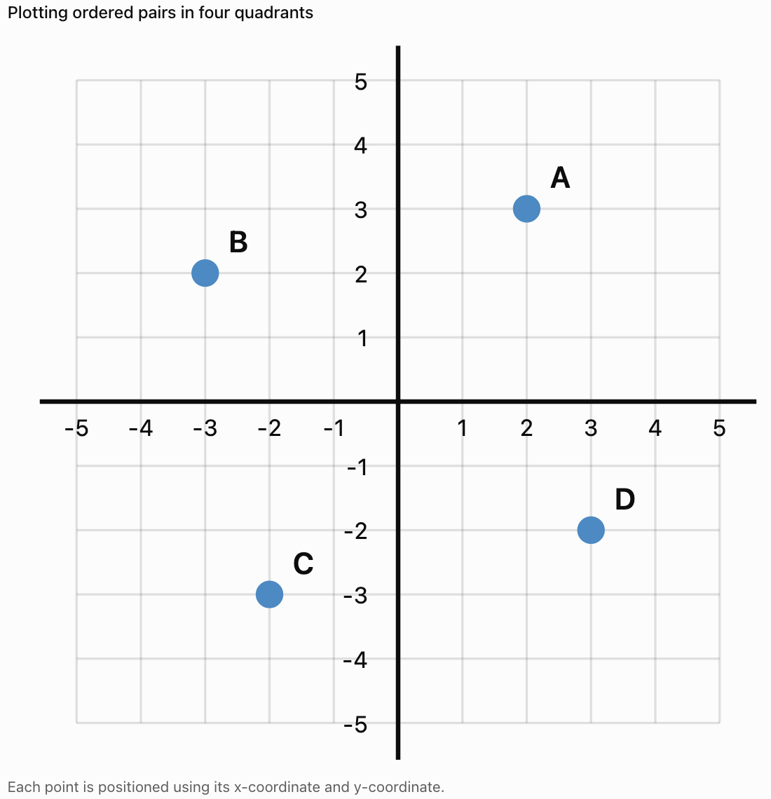
Plot the following points:
A = (2, 3)
B = (−3, 2)
C = (−2, −3)
D = (3, −2)
Important Observation
Ordered pairs provide exact locations on the coordinate plane.
What Is a Linear Relationship?
A linear relationship occurs when one variable changes at a constant rate relative to another.
Example
A student earns $5 for every hour worked.
|
Hours Worked (x) |
Earnings ($) |
|---|---|
|
0 |
0 |
|
1 |
5 |
|
2 |
10 |
|
3 |
15 |
|
4 |
20 |
Each additional hour increases earnings by $5.
This is a linear relationship.
Equation
y = 5x
where:
-
x = hours worked
-
y = total earnings
Important Observation
A constant rate of change produces a straight-line graph.
Creating Tables from Equations
A table of values can be created by substituting different x-values into an equation.
Worked Example
Consider:
y = 2x + 1
Choose the x-values:
−2, −1, 0, 1, 2
Step 1: Substitute Each Value
When x = −2:
y = 2(−2) + 1 = −3
When x = −1:
y = 2(−1) + 1 = −1
When x = 0:
y = 2(0) + 1 = 1
When x = 1:
y = 2(1) + 1 = 3
When x = 2:
y = 2(2) + 1 = 5
Step 2: Organise the Values
|
x |
y |
|---|---|
|
−2 |
−3 |
|
−1 |
−1 |
|
0 |
1 |
|
1 |
3 |
|
2 |
5 |
Step 3: Write the Ordered Pairs
(−2, −3)
(−1, −1)
(0, 1)
(1, 3)
(2, 5)
These ordered pairs can now be plotted.
Creating a Graph from a Table
Worked Example
Graph the equation:
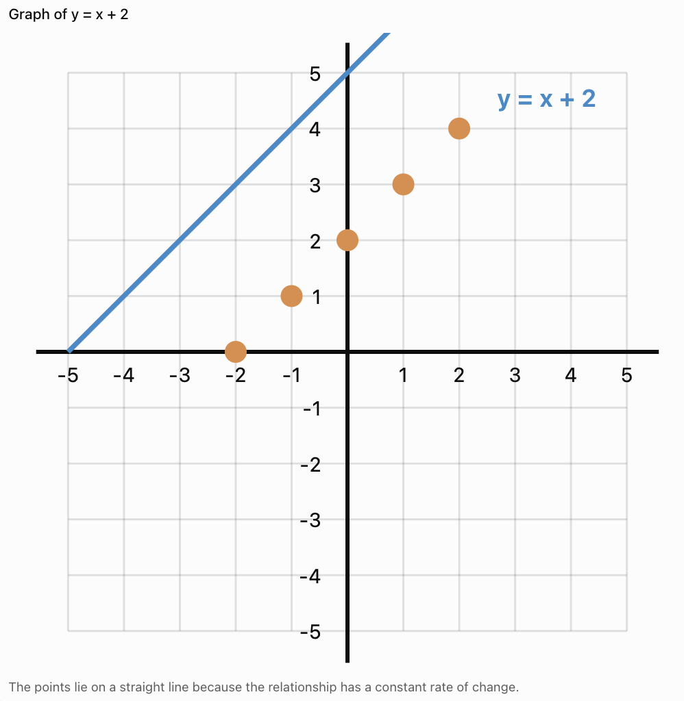
y = x + 2
Step 1: Create a Table
|
x |
y |
|---|---|
|
−2 |
0 |
|
−1 |
1 |
|
0 |
2 |
|
1 |
3 |
|
2 |
4 |
Step 2: Plot the Points
Step 3: Draw the Line
Use a ruler to draw a straight line through the points.
For a continuous linear relationship, extend the line appropriately.
Important Observation
The line represents all pairs of values satisfying the equation, not only the points originally listed in the table.
Recognising Linear Patterns in Tables
A linear relationship has a constant rate of change.
When x-values increase by equal amounts, the y-values change by equal amounts.
Example
|
x |
y |
|---|---|
|
1 |
4 |
|
2 |
7 |
|
3 |
10 |
|
4 |
13 |
|
5 |
16 |
The y-values increase by 3 each time x increases by 1.
Differences:
7 − 4 = 3
10 − 7 = 3
13 − 10 = 3
16 − 13 = 3
The rate of change is constant.
Equation
y = 3x + 1
Important Observation
A constant first difference indicates a linear relationship when the x-values are equally spaced.
Recognising Linear Patterns on Graphs
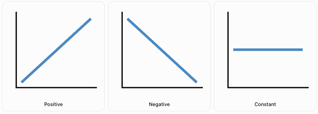
Linear relationships produce straight lines.
There are three common types of linear patterns.
Positive Linear Relationship
As x increases, y increases.
The line rises from left to right.
Negative Linear Relationship
As x increases, y decreases.
The line falls from left to right.
Constant Relationship
The y-value remains unchanged as x increases.
The line is horizontal.
Important Observation
The direction of a line reveals how the dependent variable changes as the independent variable increases.
Understanding Slope
The slope of a line measures its rate of change.
It describes how much y changes for a given change in x.
The slope is commonly represented by the letter m.
Formula
m = (y₂ − y₁)/(x₂ − x₁)
This can also be written as:
Slope = Rise / Run
where:
-
Rise = vertical change.
-
Run = horizontal change.
Worked Example
Find the slope of the line passing through:
A = (1, 3)
B = (4, 9)
Step 1: Calculate the Vertical Change
Rise = 9 − 3 = 6
Step 2: Calculate the Horizontal Change
Run = 4 − 1 = 3
Step 3: Divide
m = 6/3
m = 2
Interpretation
For every increase of 1 in x, y increases by 2.
Visualising Rise and Run
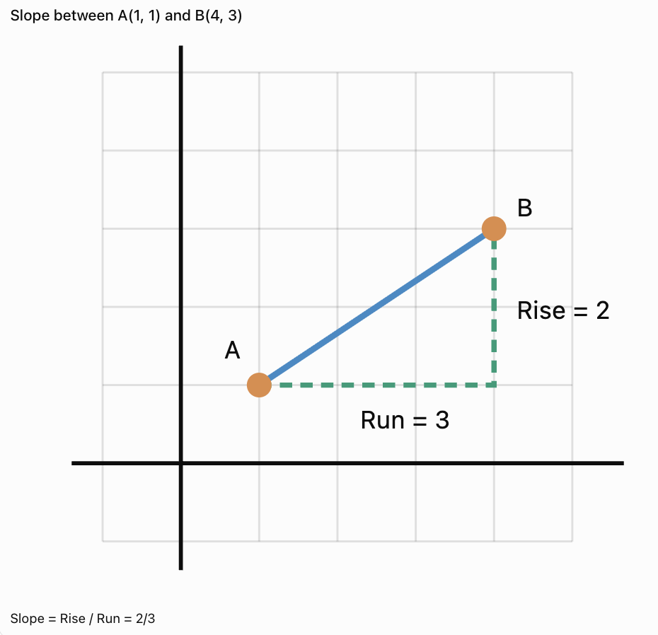
Important Observation
Slope can be positive, negative, zero, or undefined.
Positive, Negative, Zero, and Undefined Slope
Positive Slope
A line rises from left to right.
Example:
y = 2x + 1
Slope = 2
Negative Slope
A line falls from left to right.
Example:
y = −3x + 4
Slope = −3
Zero Slope
A horizontal line has slope zero.
Example:
y = 5
Slope = 0
Undefined Slope
A vertical line has an undefined slope because the horizontal change is zero.
Example:
x = 3
Important Observation
Vertical lines cannot be written in the form y = mx + b because their slope is undefined.
Slope-Intercept Form
Many linear equations can be written as:
y = mx + b
where:
-
m = slope.
-
b = y-intercept.
The y-intercept is the point where the line crosses the y-axis.
At the y-intercept:
x = 0
Example
Consider:
y = 3x + 2
Slope = 3
y-intercept = 2
The line crosses the y-axis at:
(0, 2)
Important Observation
The slope tells us how the line changes, while the y-intercept tells us where the line crosses the y-axis.
Graphing from Slope and y-Intercept
Worked Example
Graph:
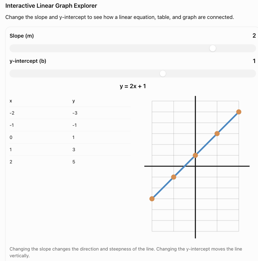
y = 2x + 1
Step 1: Identify the y-Intercept
b = 1
Plot:
(0, 1)
Step 2: Identify the Slope
m = 2
This can be written:
2/1
Move:
-
1 unit right.
-
2 units up.
Step 3: Plot Another Point
Starting at (0, 1), moving right 1 and up 2 gives:
(1, 3)
Step 4: Draw the Line
Draw a straight line through the points.
Important Observation
A straight line is uniquely determined by two distinct points.
Additional points can be used to check accuracy.
Connecting Equations, Tables, and Graphs
A linear relationship can be represented in three main ways.
Equation
y = 2x + 3
Table
|
x |
y |
|---|---|
|
0 |
3 |
|
1 |
5 |
|
2 |
7 |
|
3 |
9 |
|
4 |
11 |
Graph
The points:
(0, 3), (1, 5), (2, 7), (3, 9), (4, 11)
lie on a straight line.
How the Representations Connect
-
The equation gives the mathematical rule.
-
The table shows selected input-output values.
-
The graph displays the relationship visually.
Important Observation
All three representations describe the same relationship.
Finding an Equation from a Table
Worked Example
Determine the equation represented by the table.
|
x |
y |
|---|---|
|
0 |
4 |
|
1 |
7 |
|
2 |
10 |
|
3 |
13 |
Step 1: Find the Rate of Change
The y-values increase by 3 for every increase of 1 in x.
Therefore:
m = 3
Step 2: Find the y-Intercept
When x = 0:
y = 4
Therefore:
b = 4
Step 3: Write the Equation
y = 3x + 4
Step 4: Verify
When x = 2:
y = 3(2) + 4
y = 10
This matches the table.
Finding an Equation from Two Points
Worked Example
Find the equation of the line passing through:
(1, 4) and (3, 10)
Step 1: Calculate the Slope
m = (10 − 4)/(3 − 1)
m = 6/2
m = 3
Step 2: Use y = mx + b
y = 3x + b
Step 3: Substitute a Known Point
Using (1, 4):
4 = 3(1) + b
4 = 3 + b
b = 1
Final Equation
y = 3x + 1
Important Observation
Two distinct points determine exactly one straight line.
Interpreting Points on a Graph
Every point on a graph represents a relationship between two quantities.
Example: Distance and Time
A cyclist travels at a constant speed of 4 m/s.
The equation is:
d = 4t
where:
-
d = distance in metres.
-
t = time in seconds.
Table
|
Time (s) |
Distance (m) |
|---|---|
|
0 |
0 |
|
1 |
4 |
|
2 |
8 |
|
3 |
12 |
|
4 |
16 |
Interpreting a Point
The point (3, 12) means:
After 3 seconds, the cyclist has travelled 12 metres.
Important Observation
A graph point should always be interpreted using the quantities and units represented by the axes.
Interpreting Lines in Real-World Situations
A line represents the overall relationship between two variables.
Example: Taxi Fare
A taxi company charges:
-
A starting fee of $4.
-
An additional $2 per kilometre.
The equation is:
C = 2d + 4
where:
-
C = total cost in dollars.
-
d = distance in kilometres.
Table
|
Distance (km) |
Cost ($) |
|---|---|
|
0 |
4 |
|
1 |
6 |
|
2 |
8 |
|
3 |
10 |
|
4 |
12 |
Interpretation
The slope is 2.
This means the fare increases by $2 for each additional kilometre.
The y-intercept is 4.
This represents the starting fee.
Important Observation
The slope and y-intercept often have meaningful interpretations in practical situations.
Comparing Two Linear Relationships
Graphs can be used to compare different relationships.
Worked Example
Two companies offer delivery services.
Company A:
C = 3d + 5
Company B:
C = 2d + 9
where C is cost in dollars and d is distance in kilometres.
Table
|
Distance (km) |
Company A ($) |
Company B ($) |
|---|---|---|
|
0 |
5 |
9 |
|
1 |
8 |
11 |
|
2 |
11 |
13 |
|
3 |
14 |
15 |
|
4 |
17 |
17 |
|
5 |
20 |
19 |
Interpretation
Company A has a lower starting fee but a higher cost per kilometre.
Company B has a higher starting fee but a lower cost per kilometre.
At 4 km, both companies charge $17.
Finding the Intersection
Set the equations equal:
3d + 5 = 2d + 9
d = 4
Substitute:
C = 3(4) + 5 = 17
Intersection = (4, 17)
Important Observation
The intersection of two lines represents a point where the two relationships have the same output value for the same input.
Linear Relationships in Science
Linear relationships are common in scientific investigations.
Example: Hooke's Law
For a spring obeying Hooke's law:
F = kx
where:
-
F = force.
-
k = spring constant.
-
x = extension.
If k remains constant, force is directly proportional to extension.

Example
Suppose k = 20 N/m.
|
Extension (m) |
Force (N) |
|---|---|
|
0.00 |
0 |
|
0.05 |
1 |
|
0.10 |
2 |
|
0.15 |
3 |
|
0.20 |
4 |
The graph is a straight line through the origin.
Important Observation
A straight-line graph can reveal a constant relationship between physical quantities.
Hooke's law applies only while the spring remains within its linear elastic range.
Linear Relationships in Everyday Life
Earnings
If a worker earns $12 per hour:
E = 12h
Savings
If a person begins with $50 and saves $10 each week:
S = 10w + 50
Distance
If a vehicle travels at a constant speed of 60 km/h:
d = 60t
Water Usage
If a tank contains 200 L and loses 5 L per minute:
V = 200 − 5t
Important Observation
The slope represents a rate of change, while the intercept often represents an initial value.
When Is a Relationship Not Linear?
Not every relationship produces a straight line.
Example
Consider:
y = x²
|
x |
y |
|---|---|
|
0 |
0 |
|
1 |
1 |
|
2 |
4 |
|
3 |
9 |
|
4 |
16 |
The y-values do not increase by a constant amount.
The graph is curved.
Comparison
|
Linear |
Nonlinear |
|---|---|
|
Constant rate of change |
Changing rate of change |
|
Straight-line graph |
Often curved graph |
|
Example: y = 3x + 2 |
Example: y = x² |
|
Constant slope |
Slope may change |
Important Observation
A straight-line pattern indicates a linear relationship.
A curved graph generally indicates a nonlinear relationship.
Interpolation and Extrapolation
Linear graphs can be used to estimate unknown values.
Interpolation
Interpolation means estimating values between known data points.
Example
A cyclist travels:
-
8 m after 2 seconds.
-
16 m after 4 seconds.
Assuming constant speed, the distance after 3 seconds is:
12 m
Extrapolation
Extrapolation means predicting values beyond the known data range.
Example
If the cyclist continues at the same speed, the predicted distance after 6 seconds is:
24 m
Important Observation
Extrapolation assumes the linear pattern continues.
This may not always be realistic.
Common Mistakes
Reversing ordered pairs
Coordinates must be written (x, y).
Plotting points inaccurately
Always check both coordinate values.
Using an inconsistent scale
Graph intervals must be evenly spaced.
Confusing slope and y-intercept
Slope describes rate of change. The y-intercept describes where the line crosses the y-axis.
Forgetting negative slopes
A negative slope means y decreases as x increases.
Assuming all lines pass through the origin
Only lines with y-intercept zero pass through the origin.
Connecting points incorrectly
Linear relationships should produce straight lines.
Assuming every relationship is linear
A constant rate of change is required.
Ignoring units
Real-world graphs must include appropriate units.
Extending graphs beyond meaningful values
For example, negative time or negative distance may not make sense in a particular situation.
Misinterpreting graph intersections
An intersection represents equal output values at the same input.
Key Terms
-
Linear Relationship: Relationship with a constant rate of change.
-
Coordinate Plane: Grid used to locate points.
-
x-Axis: Horizontal axis.
-
y-Axis: Vertical axis.
-
Origin: Point (0, 0).
-
Ordered Pair: Coordinates written (x, y).
-
x-Coordinate: Horizontal position of a point.
-
y-Coordinate: Vertical position of a point.
-
Table of Values: Organised list of related input and output values.
-
Independent Variable: Input quantity, usually represented by x.
-
Dependent Variable: Output quantity, usually represented by y.
-
Slope: Rate of change of a line.
-
Rise: Vertical change between two points.
-
Run: Horizontal change between two points.
-
Positive Slope: Line rises from left to right.
-
Negative Slope: Line falls from left to right.
-
Zero Slope: Slope of a horizontal line.
-
Undefined Slope: Slope of a vertical line.
-
y-Intercept: Point where a line crosses the y-axis.
-
x-Intercept: Point where a line crosses the x-axis.
-
Slope-Intercept Form: Equation written y = mx + b.
-
Rate of Change: Change in one quantity relative to another.
-
Linear Equation: Equation whose graph is a straight line.
-
Intersection: Point where two graphs meet.
-
Interpolation: Estimating values within known data.
-
Extrapolation: Predicting values beyond known data.
-
Nonlinear Relationship: Relationship without a constant rate of change.
Key Takeaways
-
Linear relationships have a constant rate of change.
-
Linear graphs are straight lines.
-
Ordered pairs represent points on a coordinate plane.
-
Tables can be used to generate graph points.
-
Equations can be used to create tables of values.
-
The slope measures the rate of change.
-
Positive slopes rise from left to right.
-
Negative slopes fall from left to right.
-
Horizontal lines have zero slope.
-
Vertical lines have undefined slope.
-
The y-intercept is where the line crosses the y-axis.
-
Linear equations can often be written as y = mx + b.
-
Equations, tables, and graphs represent the same relationships in different ways.
-
Graph points have meaningful interpretations in real-world situations.
-
Intersections represent equal values of two relationships.
-
Linear graphs can be used to estimate and predict values.
Check Your Understanding
Plotting Ordered Pairs
-
What is an ordered pair?
-
Which coordinate is plotted first?
-
Plot the point (3, 4).
-
Plot the point (−2, 5).
-
Explain why (2, 3) and (3, 2) represent different points.
Creating Graphs from Tables
-
Create a table for y = 2x when x = 0, 1, 2, 3, 4.
-
Create a table for y = x + 3 when x = −2, −1, 0, 1, 2.
-
Write the ordered pairs from Question 7.
-
Explain how a table can be used to create a graph.
-
What shape does the graph of a linear relationship form?
Identifying Linear Patterns
-
A table contains y-values 4, 7, 10, 13, 16 for x-values 0, 1, 2, 3, 4. Is the relationship linear?
-
What is the rate of change in Question 11?
-
A line rises from left to right. Is its slope positive or negative?
-
What is the slope of a horizontal line?
-
What is the slope of a vertical line?
Interpreting Linear Relationships
-
What does the slope represent?
-
What does the y-intercept represent?
-
A taxi fare is described by C = 3d + 5. What does the number 5 represent?
-
A cyclist travels according to d = 4t. What distance is travelled after 6 seconds?
-
Explain how equations, tables, and graphs are connected.
Answer Key
|
Question |
Answer |
|---|---|
|
1 |
Pair of coordinates written (x, y) |
|
2 |
x-coordinate |
|
3 |
3 right, 4 up |
|
4 |
2 left, 5 up |
|
5 |
The coordinates are reversed |
|
6 |
y = 0, 2, 4, 6, 8 |
|
7 |
y = 1, 2, 3, 4, 5 |
|
8 |
(−2, 1), (−1, 2), (0, 3), (1, 4), (2, 5) |
|
9 |
Plot the ordered pairs and draw the appropriate graph |
|
10 |
Straight line |
|
11 |
Yes |
|
12 |
3 |
|
13 |
Positive |
|
14 |
Zero |
|
15 |
Undefined |
|
16 |
Rate of change |
|
17 |
Value of y when x = 0 |
|
18 |
Starting fee of $5 |
|
19 |
24 metres |
|
20 |
They are different representations of the same relationship |
Extended Challenge
1. Find the slope of the line passing through (2, 5) and (6, 13).
2. Determine the equation of the line passing through (0, 4) and (3, 10).
3. Create a table for y = −2x + 5 when x = 0, 1, 2, 3, 4.
4. A table shows x-values 1, 2, 3, 4 and y-values 6, 10, 14, 18. Determine the equation.
5. Find the y-intercept of y = 5x − 7.
6. Find the x-intercept of y = 2x − 8.
7. Two companies charge C = 4d + 3 and C = 2d + 11. Determine the distance at which their charges are equal.
8. A water tank contains 150 L and loses 6 L per minute. Write an equation for the water remaining after t minutes.
9. A cyclist travels at 5 m/s. Create a table showing distance travelled at 0, 2, 4, 6, and 8 seconds.
10. Explain why the relationship y = x² is nonlinear.
Extended Challenge Answers
|
Question |
Answer |
|---|---|
|
1 |
m = 2 |
|
2 |
y = 2x + 4 |
|
3 |
y = 5, 3, 1, −1, −3 |
|
4 |
y = 4x + 2 |
|
5 |
(0, −7) |
|
6 |
(4, 0) |
|
7 |
4 distance units |
|
8 |
V = 150 − 6t, for 0 ≤ t ≤ 25 |
|
9 |
0, 10, 20, 30, 40 m |
|
10 |
Its rate of change is not constant |
Final Investigation: Comparing Transportation Costs
Two transportation companies offer different pricing plans.
Company A
-
Starting fee: $5
-
Cost per kilometre: $3
Company B
-
Starting fee: $11
-
Cost per kilometre: $2
Part A: Writing Equations
-
Write an equation for Company A.
-
Write an equation for Company B.
-
Identify the slope of each equation.
-
Identify the y-intercept of each equation.
-
Explain what the slope and y-intercept represent.
Part B: Creating Tables
-
Create a table for Company A using distances 0, 1, 2, 3, 4, 5, 6, 7, and 8 km.
-
Create a table for Company B using the same distances.
-
Compare the costs at 2 km.
-
Compare the costs at 5 km.
-
Determine the distance at which both companies charge the same amount.
Part C: Graphing
-
Draw a coordinate plane.
-
Label the x-axis Distance (km).
-
Label the y-axis Cost ($).
-
Plot the points for Company A.
-
Plot the points for Company B.
-
Draw both lines and label them.
Part D: Interpreting the Graph
-
Which company has the lower starting fee?
-
Which company has the lower cost per kilometre?
-
Which company is cheaper for shorter journeys?
-
Which company is cheaper for longer journeys?
-
Explain what the intersection of the two lines represents.
-
Recommend which company a customer should choose for a journey of 10 km.
Investigation Answer Check
Equations
Company A:
C = 3d + 5
Company B:
C = 2d + 11
Tables
|
Distance (km) |
Company A ($) |
Company B ($) |
|---|---|---|
|
0 |
5 |
11 |
|
1 |
8 |
13 |
|
2 |
11 |
15 |
|
3 |
14 |
17 |
|
4 |
17 |
19 |
|
5 |
20 |
21 |
|
6 |
23 |
23 |
|
7 |
26 |
25 |
|
8 |
29 |
27 |
Intersection
3d + 5 = 2d + 11
d = 6
Cost = 3(6) + 5
Cost = $23
Both companies charge $23 for a journey of 6 km.
Comparison
-
Company A is cheaper for journeys shorter than 6 km.
-
Both companies charge the same at 6 km.
-
Company B is cheaper for journeys longer than 6 km.
10 km Journey
Company A:
C = 3(10) + 5 = $35
Company B:
C = 2(10) + 11 = $31
Company B is cheaper by $4.
Final Reflection
Graphing linear relationships allows us to connect numerical information, algebraic equations, and visual representations.
By creating tables, plotting ordered pairs, identifying linear patterns, and interpreting slopes and intercepts, we can analyse relationships and make informed predictions.
These skills are essential for solving problems involving motion, cost, growth, measurement, and many other real-world situations.
4. Slope as Rate of Change
Learning outcomes
- I can explain slope as a measure of rate of change.
- I can calculate slope from graphs and tables.
- I can compare the steepness of different lines.
- I can interpret slope in real-world contexts.
- I can explain how slope relates to linear relationships.
Slope as Rate of Change
Introduction
Imagine two cyclists travelling along a straight road.
One cyclist travels 10 metres every second, while the other travels 5 metres every second.
Both cyclists are moving at constant speeds, but the first cyclist covers distance twice as quickly.
If we graph distance against time, both cyclists produce straight lines. However, the first cyclist's line is steeper.
This illustrates one of the most important ideas in mathematics:
Slope measures the rate at which one quantity changes compared with another.
Slope is used to describe relationships involving speed, cost, temperature, population, height, and many other quantities.


What Is Slope?
The slope of a line measures how steep the line is and the direction in which it changes.
Slope is also called the gradient.
It describes how much the vertical coordinate changes compared with the horizontal coordinate.
Slope is represented by the letter m.
For a straight line:
Slope = Vertical change / Horizontal change
This is often remembered as:
Slope = Rise / Run
where:
-
Rise is the change in the y-coordinate.
-
Run is the change in the x-coordinate.
Example
Suppose a line rises 6 units while moving 3 units to the right.
Slope = 6/3
m = 2
This means that y increases by 2 units for every increase of 1 unit in x.
Important Observation
Slope describes a relationship between two changes, rather than the location of a single point.
Understanding Rise and Run
To calculate slope from a graph, identify two points on the line and determine the vertical and horizontal changes between them.
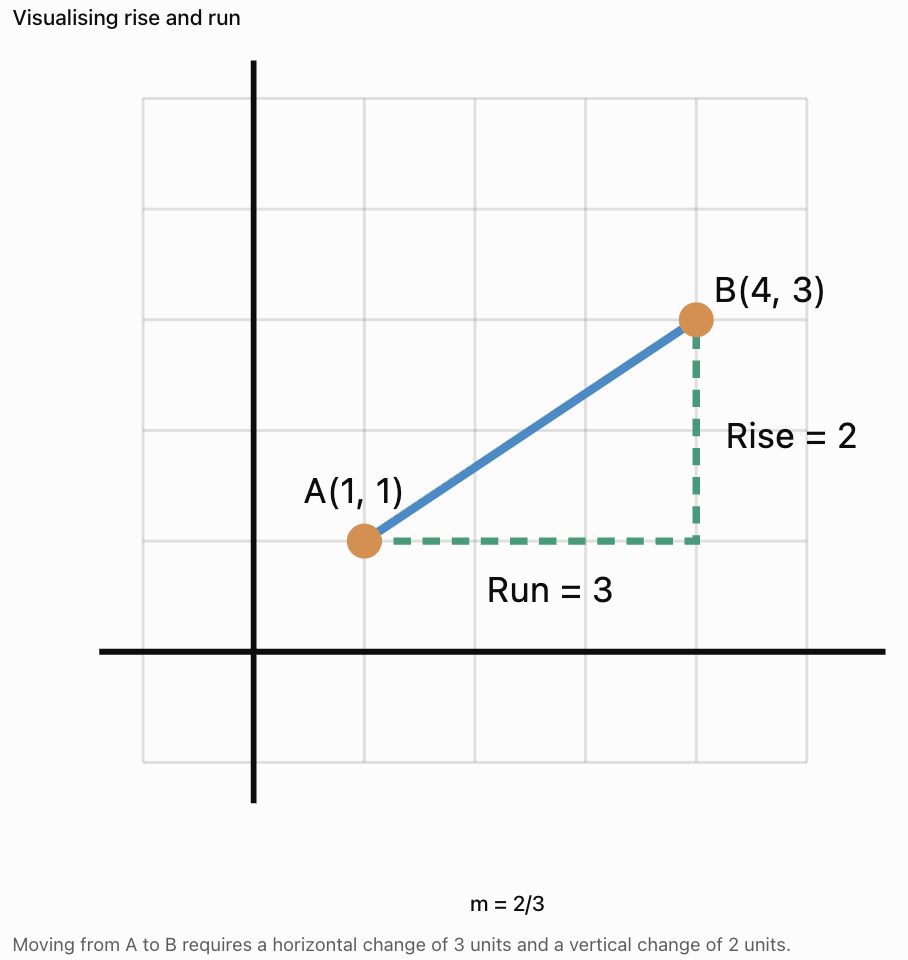
Calculation
Rise = 3 − 1 = 2
Run = 4 − 1 = 3
Slope = 2/3
m = 2/3 ≈ 0.67
Important Observation
Slope is a ratio. It does not have to be a whole number.
Calculating Slope from Two Points
If two points on a line are known, slope can be calculated using their coordinates.
Formula
m = (y₂ − y₁)/(x₂ − x₁)
where:
-
(x₁, y₁) is the first point.
-
(x₂, y₂) is the second point.
The denominator must not equal zero.
Worked Example
Find the slope of the line passing through:
A = (2, 3)
B = (6, 11)
Step 1: Identify the Coordinates
x₁ = 2
y₁ = 3
x₂ = 6
y₂ = 11
Step 2: Substitute
m = (11 − 3)/(6 − 2)
m = 8/4
m = 2
Interpretation
For every increase of 1 in x, y increases by 2.
Calculating Negative Slope
Slope can also be negative.
Worked Example
Find the slope between:
A = (1, 8)
B = (5, 2)
Step 1: Apply the Formula
m = (2 − 8)/(5 − 1)
m = −6/4
m = −3/2 = −1.5
Interpretation
For every increase of 1 in x, y decreases by 1.5.
Important Observation
A negative slope indicates a decreasing relationship as x increases.
Positive, Negative, Zero, and Undefined Slope
There are four important slope classifications.
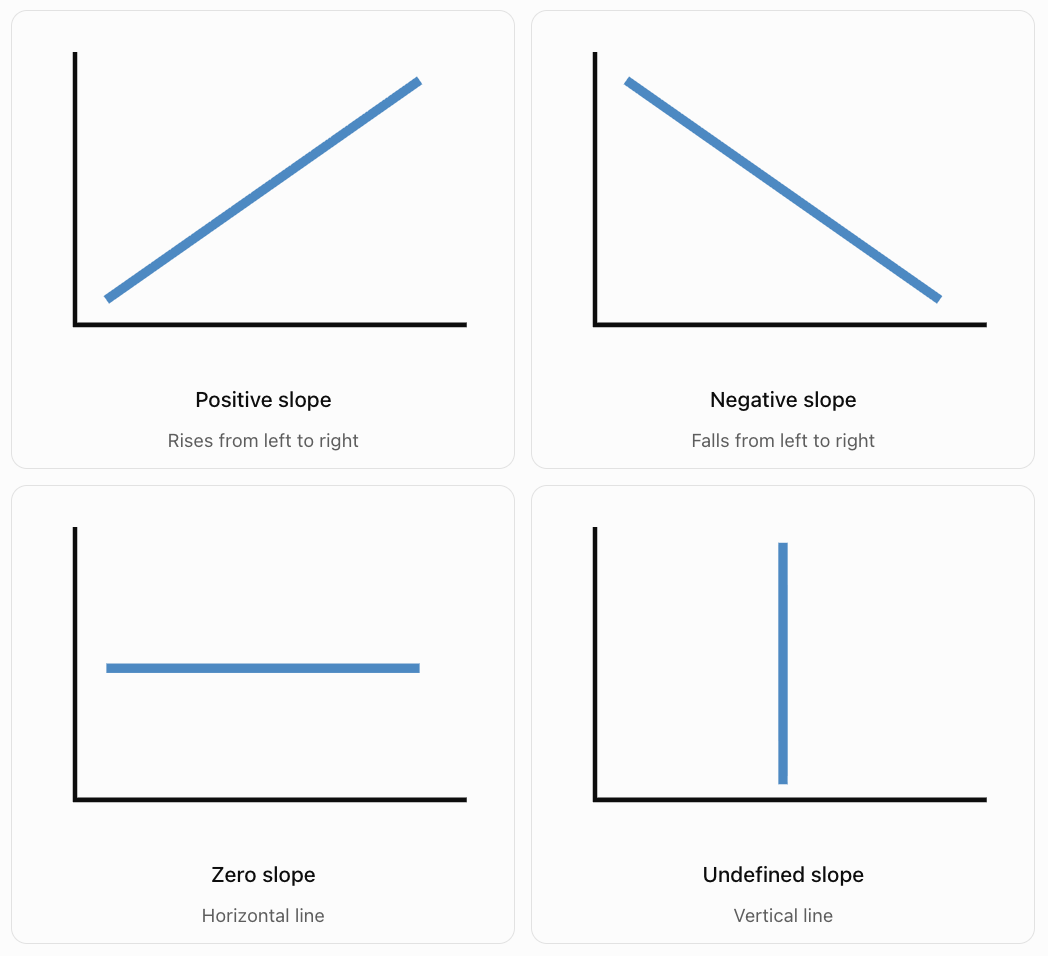
Positive Slope
A line rises from left to right.
Example:
y = 3x + 2
Slope = 3
Negative Slope
A line falls from left to right.
Example:
y = −2x + 5
Slope = −2
Zero Slope
A horizontal line has no vertical change.
Example:
y = 4
Slope = 0
Undefined Slope
A vertical line has no horizontal change.
Example:
x = 3
Slope = Undefined
Why Is Vertical Slope Undefined?
Slope = Rise / Run
For a vertical line:
Run = 0
Division by zero is undefined.
Therefore, a vertical line has an undefined slope.
Calculating Slope from a Table
Slope can be calculated using values in a table.
Worked Example
|
x |
y |
|---|---|
|
0 |
2 |
|
1 |
5 |
|
2 |
8 |
|
3 |
11 |
|
4 |
14 |
Step 1: Examine the Changes
As x increases by 1, y increases by 3.
Step 2: Calculate Slope
m = Δy/Δx
m = 3/1
m = 3
Important Observation
For a linear relationship, the ratio Δy/Δx remains constant between any two distinct points.
Tables with Unequal x-Intervals
Sometimes x-values do not increase by 1.
We must calculate the change in both variables.
Example
|
x |
y |
|---|---|
|
0 |
5 |
|
2 |
11 |
|
4 |
17 |
|
6 |
23 |
Calculation
Change in y = 11 − 5 = 6
Change in x = 2 − 0 = 2
Slope = 6/2
m = 3
Important Observation
Do not assume the slope is simply the difference between consecutive y-values.
Always compare the change in y with the corresponding change in x.
Recognising Constant Rate of Change
A linear relationship has a constant rate of change.
Example
|
Time (s) |
Distance (m) |
|---|---|
|
0 |
0 |
|
2 |
10 |
|
4 |
20 |
|
6 |
30 |
|
8 |
40 |
For each increase of 2 seconds, distance increases by 10 metres.
Slope = 10/2
m = 5 m/s
The slope is constant.
Important Observation
A constant rate of change is the defining feature of a linear relationship.
Comparing the Steepness of Lines
Slope describes how steep a line is.
For lines drawn using the same scales on both axes:
-
Larger absolute slope means a steeper line.
-
Smaller absolute slope means a less steep line.
Example
Consider three equations:
A: y = x
B: y = 2x
C: y = 4x
Their slopes are:
-
A: m = 1
-
B: m = 2
-
C: m = 4
Line C is the steepest.
Line A is the least steep.
Important Observation
The absolute value of slope determines steepness, while the sign determines whether the line rises or falls.
For example:
m = 4 and m = −4
have equal steepness but opposite directions.
Comparing Positive and Negative Slopes
Consider:
A: y = 3x + 1
B: y = −3x + 1
Both lines have slopes with absolute value 3.
Therefore, they have equal steepness when plotted using the same axis scales.
However:
-
Line A rises from left to right.
-
Line B falls from left to right.
Important Observation
A negative slope is not automatically less steep than a positive slope.
Compare absolute values when discussing steepness.
Slope and Linear Equations
Linear equations are often written in slope-intercept form:
y = mx + b
where:
-
m = slope.
-
b = y-intercept.
Example
Consider:
y = 4x + 3
The slope is:
m = 4
The y-intercept is:
b = 3
Interpretation
The line crosses the y-axis at (0, 3).
For every increase of 1 in x, y increases by 4.
Important Observation
In slope-intercept form, the coefficient of x gives the slope directly.
Slope and the y-Intercept
The slope and y-intercept describe different features of a line.
Slope
Describes how quickly y changes as x changes.
y-Intercept
Describes the value of y when x = 0.
Example
y = 5x + 20
Slope = 5
y-intercept = 20
This could represent a person who begins with $20 and saves $5 each week.
Interpretation
-
Starting savings = $20.
-
Weekly increase = $5.
Important Observation
The slope describes the rate of change, while the intercept describes the initial value.
Slope as Speed
One of the most important scientific applications of slope is motion.
On a distance-time graph:
Slope = Change in distance / Change in time
For motion in one direction at constant speed, this gives speed.

Worked Example
A cyclist travels 60 metres in 12 seconds.
Slope = 60/12
Slope = 5 m/s
Interpretation
The cyclist travels 5 metres every second.
Important Observation
A steeper distance-time line represents a greater speed when both axes use the same scales.
On a position-time graph, the slope represents velocity, which can be positive or negative.
Comparing the Speeds of Two Objects
Two cyclists travel at constant speeds.
Cyclist A
|
Time (s) |
Distance (m) |
|---|---|
|
0 |
0 |
|
2 |
12 |
|
4 |
24 |
|
6 |
36 |
Cyclist B
|
Time (s) |
Distance (m) |
|---|---|
|
0 |
0 |
|
2 |
8 |
|
4 |
16 |
|
6 |
24 |
Calculating the Slopes
Cyclist A:
m = 12/2 = 6 m/s
Cyclist B:
m = 8/2 = 4 m/s
Comparison
Cyclist A is travelling faster.
Cyclist A's distance-time graph is steeper.
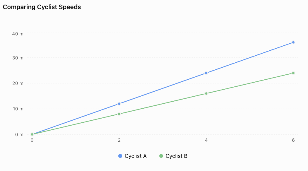
Important Observation
The graph with the greater positive slope represents the cyclist travelling faster.
Slope as a Cost per Unit
Slope can represent how much a cost changes when a quantity increases.
Example: Taxi Fare
A taxi company charges:
-
Starting fee: $4.
-
Additional charge: $3 per kilometre.
The equation is:
C = 3d + 4
where:
-
C = cost in dollars.
-
d = distance in kilometres.
Interpretation
Slope = 3 dollars per kilometre.
For every additional kilometre, the fare increases by $3.
Important Observation
Slope units are determined by dividing the units of the dependent variable by the units of the independent variable.
Here:
Slope units = dollars/km
Slope as a Rate of Heating
Scientists often use temperature-time graphs to describe heating and cooling.

Worked Example
Water temperature increases from 20°C to 50°C in 6 minutes.
Calculation
Slope = (50 − 20)/(6 − 0)
Slope = 30/6
Slope = 5°C/min
Interpretation
The water temperature increases at an average rate of 5°C per minute over the interval.
Important Observation
A positive slope indicates heating.
A negative slope indicates cooling.
A zero slope indicates constant temperature.
Slope as Population Growth
Slope can represent the rate at which a population changes.
Example
A town's population increases from 2,000 to 2,600 people over 3 years.
Slope = (2600 − 2000)/3
Slope = 600/3
Slope = 200 people/year
Interpretation
The average population increase is 200 people per year.
Important Observation
A constant population growth rate produces a linear model, although real populations often grow nonlinearly over longer periods.
Slope in Business and Finance
Businesses use slope to analyse costs, revenue, and profits.
Example
A company produces notebooks.
Its total production cost is:
C = 2n + 100
where:
-
C = total cost.
-
n = number of notebooks.
Interpretation
Slope = 2
Each additional notebook increases the total cost by $2.
y-intercept = 100
The fixed cost is $100.
Important Observation
Slope can represent marginal cost in a simple linear cost model.
Finding Slope from a Real-World Graph
Suppose a water tank is being drained.
The volume decreases from 150 L to 90 L over 10 minutes.
Step 1: Identify the Points
(0, 150)
(10, 90)
Step 2: Calculate Slope
m = (90 − 150)/(10 − 0)
m = −60/10
m = −6 L/min
Interpretation
The tank loses water at a rate of 6 litres per minute.
Important Observation
The negative sign indicates a decrease in water volume.
Parallel Lines and Slope
Two distinct nonvertical lines are parallel if they have the same slope.
Example
Line A:
y = 2x + 1
Line B:
y = 2x − 4
Both lines have slope 2.
Therefore, they are parallel.
Important Observation
Parallel lines have the same rate of change but may have different y-intercepts.
Distinct vertical lines are also parallel, even though their slopes are undefined.
Perpendicular Lines and Slope
Two nonvertical lines with nonzero slopes are perpendicular if their slopes are negative reciprocals.
Example
Line A has slope:
m₁ = 2
A perpendicular line has slope:
m₂ = −1/2
Rule
m₁ × m₂ = −1
Important Observation
A horizontal line and a vertical line are also perpendicular.
Slope and Linear Versus Nonlinear Relationships
A linear relationship has a constant slope.
A nonlinear relationship has a changing rate of change.
Example: Linear
y = 3x + 2
The slope is always 3.
Example: Nonlinear
y = x²
The slope changes depending on the position along the curve.
Comparison
|
Linear Relationship |
Nonlinear Relationship |
|---|---|
|
Constant rate of change |
Changing rate of change |
|
Straight-line graph |
Often curved graph |
|
Same slope throughout |
Slope varies |
|
Example: y = 2x + 1 |
Example: y = x² |
Important Observation
Constant slope is one of the most important ways to recognise a linear relationship.
Interactive Slope Explorer
Adjust the slope and y-intercept to investigate how the equation and graph change.
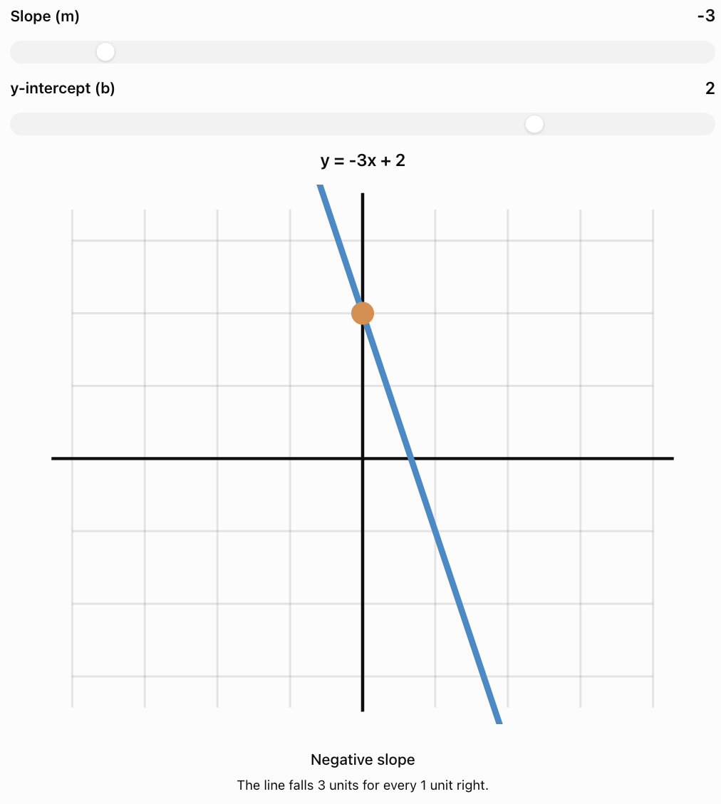
Common Mistakes
Confusing rise and run
Slope is vertical change divided by horizontal change.
Reversing the subtraction order
When calculating slope, subtract coordinates in the same order in both numerator and denominator.
Ignoring negative signs
Negative slope indicates a decreasing relationship.
Assuming negative slopes are less steep
Steepness depends on absolute slope.
Using only the change in y
Slope must account for the change in x.
Forgetting units
Real-world slopes should include appropriate units.
Confusing slope and y-intercept
Slope represents rate of change; the y-intercept represents the starting value.
Assuming every graph has a constant slope
Nonlinear graphs have changing slopes.
Treating vertical slope as zero
Vertical lines have undefined slope.
Assuming every increasing graph is linear
An increasing relationship may be nonlinear if its rate of change is not constant.
Key Terms
-
Slope: Measure of a line's steepness and rate of change.
-
Gradient: Another name for slope.
-
Rate of Change: Change in one quantity relative to another.
-
Rise: Vertical change between two points.
-
Run: Horizontal change between two points.
-
Positive Slope: Slope of a line that rises from left to right.
-
Negative Slope: Slope of a line that falls from left to right.
-
Zero Slope: Slope of a horizontal line.
-
Undefined Slope: Slope of a vertical line.
-
Linear Relationship: Relationship with constant rate of change.
-
Nonlinear Relationship: Relationship with changing rate of change.
-
Slope-Intercept Form: Equation written y = mx + b.
-
y-Intercept: Point where a line crosses the y-axis.
-
x-Intercept: Point where a line crosses the x-axis.
-
Independent Variable: Input quantity, usually x.
-
Dependent Variable: Output quantity, usually y.
-
Constant Rate of Change: Equal changes in one variable produce proportional changes in another.
-
Absolute Value: Distance of a number from zero, ignoring sign.
-
Parallel Lines: Lines in the same plane that never intersect.
-
Perpendicular Lines: Lines that intersect at right angles.
-
Distance-Time Graph: Graph showing distance as a function of time.
-
Position-Time Graph: Graph showing position as a function of time.
-
Average Rate of Change: Change in output divided by change in input over an interval.
-
Steepness: Degree to which a line rises or falls relative to the horizontal axis.
Key Takeaways
-
Slope measures the rate of change of a linear relationship.
-
Slope is calculated as rise divided by run.
-
The slope formula is m = (y₂ − y₁)/(x₂ − x₁).
-
Positive slope indicates an increasing relationship.
-
Negative slope indicates a decreasing relationship.
-
Horizontal lines have zero slope.
-
Vertical lines have undefined slope.
-
Greater absolute slope means greater steepness when the axis scales are comparable.
-
Slope can be calculated from graphs, tables, equations, and coordinates.
-
Linear relationships have constant slope.
-
Slope often represents speed, cost per unit, growth rate, or another practical quantity.
-
The units of slope are output units divided by input units.
-
In y = mx + b, m is the slope and b is the y-intercept.
-
Parallel nonvertical lines have equal slopes.
-
Perpendicular lines with defined nonzero slopes have negative reciprocal slopes.
-
Understanding slope helps us analyse and predict real-world changes.
Check Your Understanding
Understanding Slope
-
What does slope measure?
-
What is meant by rise and run?
-
Write the formula for calculating slope using two points.
-
What does a negative slope indicate?
-
What is the slope of a horizontal line?
Calculating Slope
-
Find the slope between (1, 2) and (4, 8).
-
Find the slope between (2, 7) and (6, 3).
-
Find the slope between (−3, 1) and (3, 5).
-
Find the slope of y = 4x + 7.
-
Find the slope of y = −2x − 5.
Comparing Slopes
-
Which line is steeper: m = 2 or m = 5?
-
Which line is steeper: m = −6 or m = 3?
-
What can you conclude about two distinct nonvertical lines with the same slope?
-
What is the slope of a line perpendicular to a line with slope 4?
-
Explain why a vertical line has undefined slope.
Interpreting Real-World Slopes
-
A cyclist travels 45 metres in 9 seconds at constant speed. What is the slope of the distance-time graph?
-
A water tank loses 40 litres in 8 minutes at a constant rate. What is the slope of the volume-time graph?
-
A worker earns $15 per hour. What does the slope of the earnings-time graph represent?
-
A temperature-time graph has a slope of −3°C/min. Explain its meaning.
-
Why is a constant slope important when identifying a linear relationship?
Answer Key
|
Question |
Answer |
|---|---|
|
1 |
Rate of change and steepness of a line |
|
2 |
Rise is vertical change; run is horizontal change |
|
3 |
m = (y₂ − y₁)/(x₂ − x₁) |
|
4 |
y decreases as x increases |
|
5 |
0 |
|
6 |
2 |
|
7 |
−1 |
|
8 |
2/3 |
|
9 |
4 |
|
10 |
−2 |
|
11 |
m = 5 |
|
12 |
m = −6 |
|
13 |
They are parallel |
|
14 |
−1/4 |
|
15 |
Horizontal change is zero, requiring division by zero |
|
16 |
5 m/s |
|
17 |
−5 L/min |
|
18 |
Earnings increase by $15 for each hour worked |
|
19 |
Temperature decreases by 3°C per minute |
|
20 |
A linear relationship has the same rate of change throughout |
Extended Challenge
1. Calculate the slope between A(−4, 7) and B(2, −5).
2. A line passes through (3, 8) and (7, 20). Determine its slope and equation.
3. A table contains the following values. Determine whether the relationship is linear and calculate its slope.
|
x |
y |
|---|---|
|
0 |
12 |
|
2 |
8 |
|
4 |
4 |
|
6 |
0 |
4. A straight line passes through (−2, 5) and (4, 5). Find its slope and equation.
5. Determine the slope of a line perpendicular to y = −3x + 2.
6. A vehicle's position changes from 80 m to 20 m over 12 seconds. Calculate its average velocity.
7. A company has fixed costs of $250 and an additional production cost of $8 per item. Write an equation and interpret its slope.
8. Two lines have slopes −2/3 and 4/5. Which is steeper?
9. A water tank initially contains 180 L. Its volume decreases linearly to 60 L after 15 minutes. Write an equation for the remaining volume.
10. Explain why changing the y-intercept of a line does not change its slope.
Extended Challenge Answers
|
Question |
Answer |
|---|---|
|
1 |
−2 |
|
2 |
m = 3; y = 3x − 1 |
|
3 |
Linear; m = −2 |
|
4 |
m = 0; y = 5 |
|
5 |
1/3 |
|
6 |
−5 m/s |
|
7 |
C = 8n + 250; each item adds $8 |
|
8 |
m = 4/5, because 0.8 is greater than 2/3 |
|
9 |
V = 180 − 8t, for 0 ≤ t ≤ 22.5 |
|
10 |
Changing the intercept shifts the line vertically without changing its rate of change |
Final Investigation: Comparing Rates of Change
Three students conduct investigations involving movement, temperature, and water volume.
Each investigation produces a linear relationship.
Investigation A: Motion
A toy car travels along a straight track.
|
Time (s) |
Distance (m) |
|---|---|
|
0 |
0 |
|
2 |
6 |
|
4 |
12 |
|
6 |
18 |
|
8 |
24 |
Investigation B: Heating
A container of water is heated.
|
Time (min) |
Temperature (°C) |
|---|---|
|
0 |
20 |
|
2 |
28 |
|
4 |
36 |
|
6 |
44 |
|
8 |
52 |
Investigation C: Draining Water
Water drains from a tank.
|
Time (min) |
Volume (L) |
|---|---|
|
0 |
100 |
|
2 |
90 |
|
4 |
80 |
|
6 |
70 |
|
8 |
60 |
Part A: Calculating Slopes
-
Calculate the slope of Investigation A.
-
State the units of this slope.
-
Explain what the slope represents.
-
Calculate the slope of Investigation B.
-
State the units of this slope.
-
Calculate the slope of Investigation C.
-
Explain why the slope of Investigation C is negative.
Part B: Creating Graphs
-
Draw a separate coordinate graph for each investigation.
-
Label the horizontal and vertical axes.
-
Choose appropriate scales.
-
Plot the ordered pairs.
-
Draw straight lines through the points.
-
Identify which graphs have positive slopes.
-
Identify which graph has a negative slope.
Part C: Writing Equations
-
Write an equation describing the toy car's distance.
-
Write an equation describing the water temperature.
-
Write an equation describing the tank's remaining water volume.
-
Use the equations to predict the values after 10 units of time, using the appropriate time units for each investigation.
Part D: Evaluating Relationships
-
Explain why all three relationships are linear.
-
Explain why it is not meaningful to compare the numerical steepness of these three graphs without considering their different units and axis scales.
Investigation Answer Check
Investigation A
Slope = (24 − 0)/(8 − 0)
m = 3 m/s
Equation:
d = 3t
After 10 seconds:
d = 3 × 10 = 30 m
Investigation B
Slope = (52 − 20)/(8 − 0)
m = 4°C/min
Equation:
T = 4t + 20
After 10 minutes:
T = 4(10) + 20 = 60°C
Investigation C
Slope = (60 − 100)/(8 − 0)
m = −5 L/min
Equation:
V = 100 − 5t
After 10 minutes:
V = 100 − 5(10) = 50 L
Final Reflection
Slope provides a mathematical way to describe how quickly quantities change.
It can be calculated from graphs, tables, equations, and coordinates, and it has important meanings in real-world situations.
Understanding slope allows us to compare rates of change, recognise linear relationships, interpret scientific data, and make predictions.
The central principle is that a linear relationship has a constant rate of change, represented by the slope of its straight-line graph.
5. Algebraic Modeling Project
Learning outcomes
- I can create equations to represent real-world situations.
- I can generate tables of values from equations.
- I can graph relationships accurately.
- I can analyze and interpret mathematical models.
- I can communicate findings using equations, graphs, and written explanations.
Algebraic Modeling Project
Introduction to Algebraic Modeling
Mathematics is more than solving equations. It is also a powerful tool for understanding the world around us.
Algebraic modeling is the process of representing real-world situations using variables, equations, tables, and graphs.
A mathematical model allows us to describe relationships, investigate patterns, make predictions, and compare possible solutions.
For example, algebraic models can help us answer questions such as:
-
How much money will I save after several months?
-
Which mobile phone plan offers better value?
-
How far will a vehicle travel at a constant speed?
-
How many products must a business sell to make a profit?
-
How does the amount of water in a tank change over time?
-
How can we predict future costs from existing data?
In an algebraic modeling project, we begin with a real-world problem and develop a mathematical representation of the situation.


The goal is not simply to produce an equation. A successful mathematical model should also be understandable, useful, and appropriate for the situation being investigated.
What Is a Mathematical Model?
A mathematical model is a representation of a real-world system using mathematical relationships.
Models may include:
-
Equations
-
Tables
-
Graphs
-
Diagrams
-
Inequalities
-
Functions
-
Written explanations
Example: Saving Money
Suppose a student already has $50 and saves an additional $10 each week.
After one week:
Savings = 50 + 10 = $60
After two weeks:
Savings = 50 + 20 = $70
After three weeks:
Savings = 50 + 30 = $80
We can describe the situation using an equation:
S = 10w + 50
where:
-
S = total savings in dollars.
-
w = number of weeks.
This equation is a mathematical model.
It allows us to calculate savings for any number of weeks, assuming the student continues saving at the same rate.
Important Observation
A mathematical model simplifies reality so that important relationships can be studied.
The Algebraic Modeling Process
A useful modeling process follows a series of connected stages.
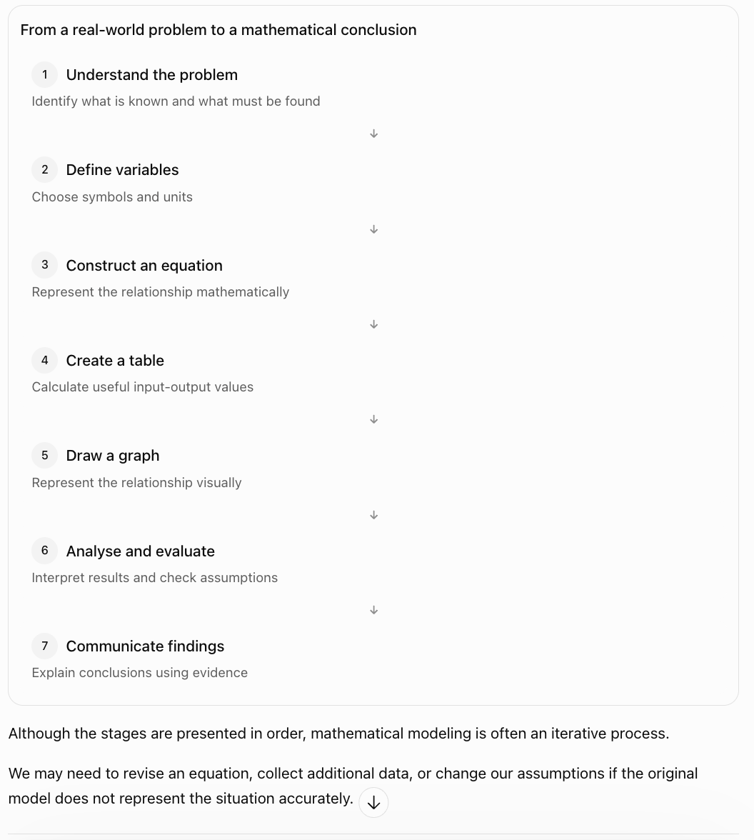
Although the stages are presented in order, mathematical modeling is often an iterative process.
We may need to revise an equation, collect additional data, or change our assumptions if the original model does not represent the situation accurately.
Identifying Variables
Variables represent quantities that can change.
Two important types are independent and dependent variables.
Independent Variable
The independent variable is the input quantity.
It is often represented by x.
Examples include:
-
Time
-
Distance travelled
-
Number of items purchased
-
Number of hours worked
Dependent Variable
The dependent variable is the output quantity.
It is often represented by y.
Examples include:
-
Total cost
-
Earnings
-
Distance travelled
-
Amount of money saved
Example: Buying Notebooks
A notebook costs $4.
The total cost depends on the number of notebooks purchased.
Independent variable: Number of notebooks, n
Dependent variable: Total cost, C
The equation is:
C = 4n
Important Observation
The dependent variable changes according to the value of the independent variable.
Creating Equations from Real-World Situations
One of the most important modeling skills is translating words into algebra.
Example: Gym Membership
A gym charges:
-
A registration fee of $30.
-
A monthly membership fee of $20.
Let:
m = number of months
C = total cost in dollars
The total cost consists of two parts:
Total cost = Monthly cost + Registration fee
Therefore:
C = 20m + 30
Interpretation
The coefficient 20 represents the monthly charge.
The constant 30 represents the initial registration fee.
Important Observation
Many real-world linear models can be written as:
y = mx + b
where:
-
m = rate of change.
-
b = initial value.
Understanding Initial Values and Rates of Change
In the equation:
y = mx + b
the two most important quantities are the slope and y-intercept.
Slope
The slope represents how much the output changes for each unit increase in the input.
y-Intercept
The y-intercept represents the output when the input equals zero.
Worked Example
A water tank initially contains 200 litres of water.
Water drains at a constant rate of 8 litres per minute.
Let:
t = time in minutes
V = volume of water in litres
The equation is:
V = 200 − 8t
Interpretation
-
Initial volume = 200 L.
-
Rate of change = −8 L/min.
-
The negative slope indicates decreasing volume.
Important Observation
A negative rate of change often represents a decrease, such as water loss, cooling, or spending savings.
Creating Tables of Values
Once an equation has been constructed, we can generate a table by substituting different values of the independent variable.
Worked Example: Gym Membership
Equation:
C = 20m + 30
Calculate the cost for 0–5 months.
|
Months (m) |
Calculation |
Total Cost ($) |
|---|---|---|
|
0 |
20(0) + 30 |
30 |
|
1 |
20(1) + 30 |
50 |
|
2 |
20(2) + 30 |
70 |
|
3 |
20(3) + 30 |
90 |
|
4 |
20(4) + 30 |
110 |
|
5 |
20(5) + 30 |
130 |
Important Observation
Each row of the table shows a possible situation described by the equation.
Converting Tables into Ordered Pairs
To graph a relationship, each row can be written as an ordered pair.
For the gym membership model:
(0, 30)
(1, 50)
(2, 70)
(3, 90)
(4, 110)
(5, 130)
The first coordinate represents the number of months.
The second coordinate represents the total cost.
Important Observation
The meaning of each coordinate depends on the variables being modeled.
Graphing a Mathematical Model
A graph provides a visual representation of a mathematical relationship.
Steps for Creating an Accurate Graph
-
Draw a coordinate plane.
-
Label the horizontal axis with the independent variable.
-
Label the vertical axis with the dependent variable.
-
Include appropriate units.
-
Choose a consistent scale.
-
Plot the ordered pairs accurately.
-
Draw the appropriate line or curve.
-
Include a descriptive title.
Example: Gym Membership
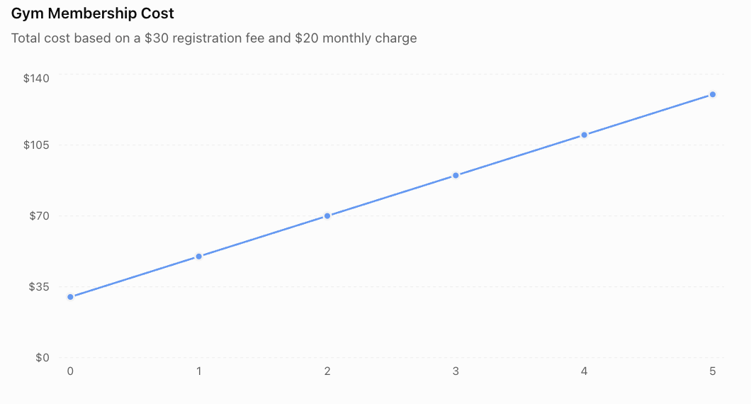
Interpreting the Graph
The graph is a straight line.
The slope is positive because the total cost increases each month.
The y-intercept is $30, representing the registration fee.
Important Observation
A graph makes the pattern of increasing cost easier to recognise.
Choosing Appropriate Graph Scales
The scale of a graph determines how values are displayed.
A good scale should:
-
Include all relevant values.
-
Use consistent intervals.
-
Be easy to read.
-
Avoid unnecessary empty space.
-
Clearly show important changes.
Example
Suppose total costs range from $30 to $130.
A reasonable vertical scale might increase by $20 per major interval.
An unsuitable scale might increase by $1 per major interval, requiring a very large graph.
Important Observation
Poorly chosen scales can make graphs difficult to interpret or create misleading visual impressions.
Interpreting Mathematical Models
A model is useful only if its mathematical results can be explained in the context of the original situation.
Worked Example: Water Tank
Equation:
V = 200 − 8t
where:
-
V = water volume in litres.
-
t = time in minutes.
Question: How Much Water Remains After 10 Minutes?
V = 200 − 8(10)
V = 200 − 80
V = 120 L
Question: When Will the Tank Be Empty?
Set V = 0.
0 = 200 − 8t
8t = 200
t = 25 minutes
Interpretation
If the draining rate remains constant, the tank will be empty after 25 minutes.
Important Observation
The model is meaningful only while the tank contains water.
The physical domain is:
0 ≤ t ≤ 25
Negative water volumes are not physically meaningful.
The Importance of Assumptions
A mathematical model often depends on assumptions.
An assumption is a condition accepted as true for the purpose of simplifying a problem.
Example: Water Tank
The equation:
V = 200 − 8t
assumes that:
-
The initial volume is exactly 200 L.
-
Water drains at a constant rate.
-
No additional water enters the tank.
-
There are no leaks other than the modeled outflow.
If these conditions change, the model may no longer be accurate.
Important Observation
A mathematical model is only as useful as its assumptions and the quality of its data.
Comparing Two Mathematical Models
One of the most useful applications of algebraic modeling is comparing alternatives.
Worked Example: Two Mobile Phone Plans
A customer is choosing between two plans.
Plan A
-
Monthly base fee: $15.
-
Additional cost: $4 per GB of data.
Plan B
-
Monthly base fee: $35.
-
Additional cost: $2 per GB of data.

Step 1: Define Variables
d = data used in GB
C = monthly cost in dollars
Step 2: Write Equations
Plan A:
Cₐ = 4d + 15
Plan B:
Cᵦ = 2d + 35
Step 3: Create a Table
|
Data (GB) |
Plan A ($) |
Plan B ($) |
|---|---|---|
|
0 |
15 |
35 |
|
5 |
35 |
45 |
|
10 |
55 |
55 |
|
15 |
75 |
65 |
|
20 |
95 |
75 |
Step 4: Graph the Relationships
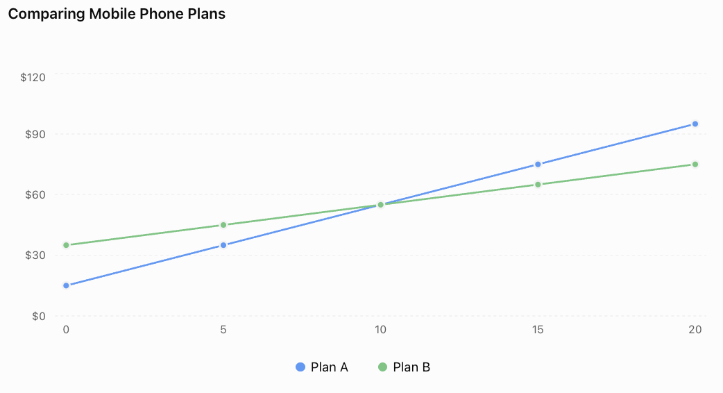
Step 5: Find the Break-Even Point
At the break-even point, both plans have the same cost.
4d + 15 = 2d + 35
2d = 20
d = 10 GB
Substitute:
C = 4(10) + 15
C = $55
Conclusion
-
Plan A is cheaper below 10 GB.
-
Both plans cost the same at 10 GB.
-
Plan B is cheaper above 10 GB.
Important Observation
The intersection of two linear models represents a situation where both produce the same output.
Interpolation and Extrapolation
Mathematical models can be used to estimate unknown values.
Interpolation
Interpolation estimates values within the range of known data.
For example, if a table records costs at 5 GB and 10 GB, a model can estimate the cost at 7 GB.
Extrapolation
Extrapolation estimates values outside the known data range.
For example, a model based on data usage up to 20 GB might be used to predict the cost at 30 GB.
Important Observation
Extrapolation is less reliable when conditions may change outside the observed range.
A mobile provider might introduce additional charges, discounts, or data limits.
Evaluating Model Accuracy
A mathematical model should be checked against real data whenever possible.
Example: Predicted and Actual Sales
A shop predicts weekly sales using:
S = 20w + 100
where:
-
S = predicted sales.
-
w = number of weeks.
Suppose the actual sales are:
|
Week |
Predicted Sales |
Actual Sales |
|---|---|---|
|
0 |
100 |
102 |
|
1 |
120 |
118 |
|
2 |
140 |
145 |
|
3 |
160 |
157 |
|
4 |
180 |
184 |
The model is reasonably close to the observed data, but it is not exact.
Calculating Prediction Error
For week 2:
Predicted sales = 140
Actual sales = 145
Error = Actual − Predicted
Error = 145 − 140
Error = 5
The model underestimated sales by 5 units.
Important Observation
Differences between predicted and observed values help us evaluate the accuracy of a model.
Residuals and Model Evaluation
A residual is the difference between an observed value and the value predicted by a model.
Residual = Observed value − Predicted value
Example
A model predicts a temperature of 28°C.
The actual measured temperature is 30°C.
Residual = 30 − 28
Residual = +2°C
A positive residual means the observed value is higher than predicted.
A negative residual means the observed value is lower than predicted.
Important Observation
Patterns in residuals can indicate that a model does not adequately describe the data.
For example, consistently curved residual patterns may suggest that a nonlinear model would be more appropriate.
Linear and Nonlinear Models
Not every real-world relationship is linear.
Linear Model
A linear model has a constant rate of change.
Example:
C = 5n + 20
The cost increases by $5 for each additional item.
Nonlinear Model
A nonlinear model has a changing rate of change.
Example:
A = s²
The area of a square depends on the square of its side length.
|
Side Length (cm) |
Area (cm²) |
|---|---|
|
1 |
1 |
|
2 |
4 |
|
3 |
9 |
|
4 |
16 |
|
5 |
25 |
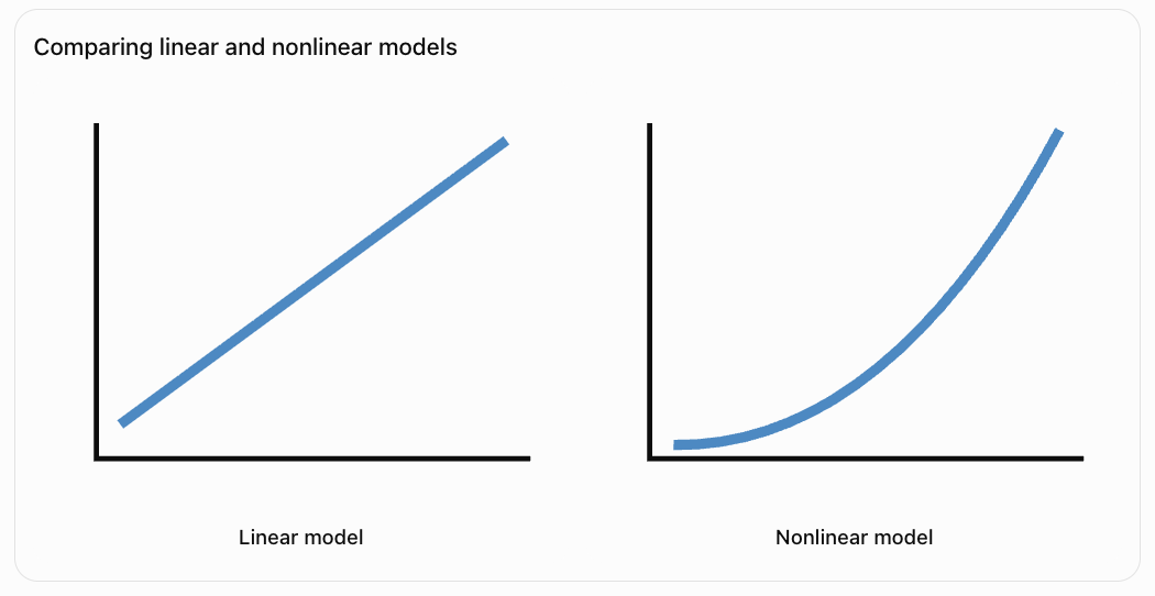
Important Observation
The type of equation should match the behaviour of the real-world situation.
Modeling with Inequalities
Some real-world problems involve restrictions rather than exact values.
Example: Budgeting
A student has $100 to spend on notebooks.
Each notebook costs $8.
Let n = number of notebooks.
The total cost must not exceed $100.
8n ≤ 100
Solving:
n ≤ 12.5
Because notebooks are purchased in whole numbers:
Maximum number of notebooks = 12
Important Observation
Inequalities are useful for modeling budgets, limits, capacities, and other constraints.
Modeling with Multiple Constraints
Some situations involve several restrictions.
Example: School Event
A school is planning a trip.
Each student ticket costs $12.
The school has a budget of $360.
The bus can carry a maximum of 25 students.
Let n = number of students.
Budget constraint:
12n ≤ 360
Therefore:
n ≤ 30
Bus capacity constraint:
n ≤ 25
Both constraints must be satisfied.
Conclusion
Maximum number of students = 25
Important Observation
A valid mathematical solution must satisfy every relevant constraint.
Mathematical Modeling in Science
Mathematical models are widely used to describe scientific relationships.
Example: Constant Speed
For motion at constant speed:
d = vt
where:
-
d = distance.
-
v = speed.
-
t = time.
If v = 6 m/s:
d = 6t

Table
|
Time (s) |
Distance (m) |
|---|---|
|
0 |
0 |
|
2 |
12 |
|
4 |
24 |
|
6 |
36 |
|
8 |
48 |
Interpretation
The slope of the distance-time graph is 6 m/s.
The model assumes the object travels at a constant speed.
Important Observation
Scientific models connect mathematical equations to measurable physical quantities.
Mathematical Modeling in Business
Businesses use mathematical models to predict costs, revenue, and profit.
Example
A company sells reusable water bottles.
Selling price per bottle = $15
Variable production cost per bottle = $6
Fixed costs = $180
Revenue Model
R = 15n
Cost Model
C = 6n + 180
Profit Model
Profit = Revenue − Cost
P = 15n − (6n + 180)
P = 9n − 180
Break-Even Point
Set profit equal to zero.
0 = 9n − 180
9n = 180
n = 20
The company must sell 20 bottles to break even.
Important Observation
Algebraic models help businesses determine how many products must be sold before profit begins.
Communicating Mathematical Findings
A successful modeling project should communicate more than calculations.
A complete explanation should include:
-
The real-world problem.
-
Definitions of variables.
-
The mathematical equation.
-
A table of values.
-
An accurately labelled graph.
-
Calculations and predictions.
-
Interpretation of slope and intercepts.
-
Assumptions and limitations.
-
A clear conclusion.
Example of a Mathematical Conclusion
A student investigates a savings plan described by:
S = 15w + 40
A suitable conclusion would be:
"The model shows that the student begins with $40 and saves an additional $15 each week. The graph is linear because the savings increase at a constant rate. After 12 weeks, the predicted savings are $220. This prediction assumes the student continues saving the same amount each week."
Important Observation
Mathematical communication should explain what the numbers mean, not simply present the numbers.
Interactive Algebraic Model Explorer
Explore a simple cost model by adjusting the cost per item and fixed starting cost.
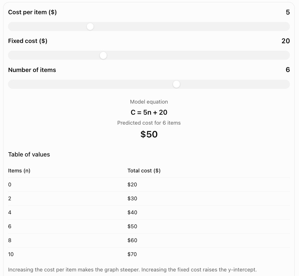
Common Mistakes
Using variables without defining them
Every variable should have a clear meaning and appropriate units.
Confusing fixed costs and variable costs
Fixed costs do not depend on the quantity produced, while variable costs change with quantity.
Writing an incorrect equation
Check that the equation matches the information given in the problem.
Reversing independent and dependent variables
The independent variable is usually placed on the x-axis.
Creating inaccurate tables
Substitute values carefully and check calculations.
Using inconsistent graph scales
Graph intervals should be evenly spaced and clearly labelled.
Ignoring units
Mathematical results should include appropriate units.
Interpreting slope incorrectly
Slope represents the rate of change, not necessarily the starting value.
Ignoring realistic restrictions
Negative quantities or fractional people may not make sense in a practical model.
Assuming every model is linear
Some real-world relationships require nonlinear equations.
Extrapolating too far
Predictions outside the observed range may be unreliable.
Presenting calculations without explanations
A mathematical model should be interpreted in the context of the problem.
Key Terms
-
Algebraic Modeling: Representing real-world situations using algebraic relationships.
-
Mathematical Model: Mathematical representation of a real-world system.
-
Variable: Symbol representing a quantity that can change.
-
Independent Variable: Input quantity.
-
Dependent Variable: Output quantity.
-
Equation: Mathematical statement expressing equality.
-
Linear Equation: Equation representing a straight-line relationship.
-
Nonlinear Equation: Equation representing a relationship without constant rate of change.
-
Slope: Rate of change of a linear relationship.
-
y-Intercept: Output value when the input equals zero.
-
Initial Value: Starting quantity in a model.
-
Fixed Cost: Cost that remains unchanged as output changes within a specified range.
-
Variable Cost: Cost that changes with production or usage.
-
Table of Values: Organised list of related input and output values.
-
Ordered Pair: Pair of values written (x, y).
-
Graph: Visual representation of a mathematical relationship.
-
Domain: Set of allowed input values.
-
Range: Set of possible output values.
-
Constraint: Restriction placed on a mathematical model.
-
Assumption: Condition accepted as true when constructing a model.
-
Interpolation: Estimating values within a known data range.
-
Extrapolation: Estimating values outside a known data range.
-
Prediction: Estimate produced using a mathematical model.
-
Residual: Difference between an observed value and a predicted value.
-
Revenue: Money received from sales.
-
Profit: Revenue minus total cost.
-
Break-Even Point: Point where revenue equals cost.
-
Model Accuracy: How closely model predictions match real observations.
-
Model Limitation: Condition restricting the usefulness or accuracy of a model.
-
Mathematical Communication: Explaining mathematical ideas and results clearly using equations, graphs, tables, and written reasoning.
Key Takeaways
-
Algebraic modeling connects mathematics to real-world situations.
-
Models can include equations, tables, graphs, and written explanations.
-
Variables should be clearly defined.
-
Linear models have constant rates of change.
-
The slope represents the rate at which the output changes.
-
The y-intercept often represents an initial value.
-
Tables allow us to calculate and organise model values.
-
Graphs provide visual representations of relationships.
-
Intersections can represent break-even points or equal costs.
-
Models can be used to make predictions.
-
Realistic constraints must be considered.
-
Assumptions affect model accuracy.
-
Predictions should be checked against available evidence.
-
A successful model must be mathematically correct and meaningful in context.
-
Clear communication is an essential part of mathematical modeling.
Check Your Understanding
Creating Equations
-
What is algebraic modeling?
-
Why are variables important in mathematical models?
-
A student saves $8 each week and begins with $25. Write an equation for total savings.
-
A taxi charges $5 plus $3 per kilometre. Write an equation for the total fare.
-
A tank contains 150 L and loses 6 L per minute. Write an equation for the remaining water.
Creating Tables
-
Create a table for y = 2x + 3 when x = 0, 1, 2, 3, 4.
-
Create a table for C = 5n + 20 when n = 0, 2, 4, 6.
-
Explain how a table can be used to generate graph points.
-
What is an ordered pair?
-
Why should tables include units?
Graphing and Interpreting
-
What does the slope represent in y = 4x + 10?
-
What does the y-intercept represent in a cost model?
-
A graph shows total cost increasing by $6 per item. What is the slope?
-
What does the intersection of two cost graphs represent?
-
Why should graph axes be labelled?
Evaluating Models
-
What is an assumption?
-
Why should realistic constraints be considered?
-
What is the difference between interpolation and extrapolation?
-
How can a model be checked for accuracy?
-
Why is written explanation important in a mathematical project?
Answer Key
|
Question |
Answer |
|---|---|
|
1 |
Representing real-world situations mathematically |
|
2 |
They represent quantities that change |
|
3 |
S = 8w + 25 |
|
4 |
C = 3d + 5 |
|
5 |
V = 150 − 6t |
|
6 |
y = 3, 5, 7, 9, 11 |
|
7 |
C = 20, 30, 40, 50 |
|
8 |
Each row provides an ordered pair |
|
9 |
Pair of related values written (x, y) |
|
10 |
To identify measurement quantities |
|
11 |
Output increases by 4 per unit increase in x |
|
12 |
Initial or fixed cost |
|
13 |
6 dollars per item |
|
14 |
Equal costs at the same input |
|
15 |
To identify quantities and units |
|
16 |
Condition accepted as true for modeling |
|
17 |
To ensure solutions are realistic |
|
18 |
Interpolation estimates within the data range; extrapolation estimates beyond it |
|
19 |
Compare predictions with observed data |
|
20 |
To explain the meaning and limitations of results |
Extended Challenge
1. A company charges $12 per month plus $5 per service. Write an equation for total monthly cost.
2. A water tank contains 240 L and drains at 12 L/min. Determine when it becomes empty.
3. A business sells products for $18 each. Fixed costs are $300 and variable costs are $8 per item. Write equations for revenue, cost, and profit.
4. Determine the break-even quantity for Question 3.
5. Two companies charge C₁ = 4x + 25 and C₂ = 6x + 5. Determine when their costs are equal.
6. A student saves $15 per week, beginning with $60. How many weeks are required to reach $300?
7. A model predicts 120 customers, but 135 customers actually visit. Calculate the residual.
8. A rectangle has width x and length x + 3. Write an equation for its area.
9. Explain why the model in Question 8 is nonlinear.
10. Explain why a model may produce mathematically correct results that are unrealistic in the real world.
Extended Challenge Answers
|
Question |
Answer |
|---|---|
|
1 |
C = 5s + 12, where s is number of services |
|
2 |
20 minutes |
|
3 |
R = 18n; C = 8n + 300; P = 10n − 300 |
|
4 |
30 items |
|
5 |
x = 10; both cost $65 |
|
6 |
16 weeks |
|
7 |
+15 customers |
|
8 |
A = x(x + 3) = x² + 3x |
|
9 |
The equation contains x² and has a changing rate of change |
|
10 |
Models may ignore physical constraints or depend on unrealistic assumptions |
Final Project: Planning a School Fundraising Event
A school wants to raise money by selling tickets to a student concert.
The organisers must decide how many tickets need to be sold to cover costs and generate a profit.
Project Information
The event has the following costs:
-
Venue rental: $250
-
Equipment rental: $150
-
Advertising: $100
-
Additional cost per attendee: $2
Each ticket sells for $12.
Part A: Understanding the Situation
-
Identify the fixed costs.
-
Calculate the total fixed cost.
-
Identify the variable cost per attendee.
-
Identify the selling price per ticket.
-
Define appropriate variables.
Part B: Constructing Equations
-
Write an equation for total revenue.
-
Write an equation for total cost.
-
Write an equation for profit.
-
Explain the meaning of the slope in the revenue model.
-
Explain the meaning of the y-intercept in the cost model.
Part C: Creating Tables
-
Create a table for 0, 20, 40, 60, 80, and 100 tickets sold.
-
Calculate revenue for each quantity.
-
Calculate cost for each quantity.
-
Calculate profit for each quantity.
Part D: Graphing the Models
-
Draw a coordinate plane.
-
Label the x-axis Number of Tickets Sold.
-
Label the y-axis Amount ($).
-
Plot the revenue model.
-
Plot the cost model.
-
Identify the intersection.
Part E: Analysing Results
-
Determine the break-even number of tickets.
-
Calculate the profit from selling 80 tickets.
-
Calculate the profit from selling 120 tickets.
-
Determine the minimum number of tickets required to earn at least $500 profit.
-
Explain how the results could help the school plan the event.
Part F: Communicating Findings
Prepare a short mathematical report that includes:
-
A description of the fundraising problem.
-
Definitions of variables.
-
Revenue, cost, and profit equations.
-
A completed table of values.
-
A graph comparing revenue and cost.
-
Calculations showing the break-even point.
-
A recommendation for a realistic ticket-sales target.
-
An explanation of assumptions and limitations.
Project Answer Check
Fixed Costs
250 + 150 + 100 = $500
Revenue Equation
R = 12n
Cost Equation
C = 2n + 500
Profit Equation
P = R − C
P = 12n − (2n + 500)
P = 10n − 500
Completed Table
|
Tickets Sold |
Revenue ($) |
Cost ($) |
Profit ($) |
|---|---|---|---|
|
0 |
0 |
500 |
−500 |
|
20 |
240 |
540 |
−300 |
|
40 |
480 |
580 |
−100 |
|
60 |
720 |
620 |
100 |
|
80 |
960 |
660 |
300 |
|
100 |
1200 |
700 |
500 |
Break-Even Point
Set revenue equal to cost.
12n = 2n + 500
10n = 500
n = 50 tickets
The school must sell 50 tickets to break even.
Profit from 80 Tickets
P = 10(80) − 500
P = $300
Profit from 120 Tickets
P = 10(120) − 500
P = $700
Tickets Required for $500 Profit
10n − 500 ≥ 500
10n ≥ 1000
n ≥ 100
The school must sell at least 100 tickets.
Evaluating the Model
The model assumes that:
-
Every ticket sells for $12.
-
Every attendee incurs an additional cost of $2.
-
Fixed costs remain unchanged.
-
All tickets sold correspond to paying attendees.
-
The venue can accommodate the expected number of students.
If the venue has a maximum capacity of 90 students, a profit of $500 would not be achievable under the existing pricing model.
Example Conclusion
The algebraic model shows that the concert must sell at least 50 tickets to cover its costs. Selling 80 tickets would generate a profit of $300, while selling 100 tickets would generate $500. The school should aim to sell at least 100 tickets if the venue capacity allows. The model is useful for planning, but actual results may differ if expenses change or ticket sales are lower than expected.
Final Reflection
Algebraic modeling connects mathematical knowledge with practical decision-making.
By creating equations, generating tables, constructing graphs, and interpreting results, we can investigate complex situations using clear mathematical reasoning.
A successful modeling project should not simply produce calculations. It should explain what the calculations mean, evaluate the assumptions involved, and communicate useful conclusions.
The most important principle is that mathematics becomes especially powerful when equations, tables, graphs, and written explanations are used together to understand real-world problems.