Tables and Graphs

Introduction

Tables and graphs are important tools for organising, representing, and interpreting information.

A table arranges data into rows and columns, making it easier to identify values, compare quantities, and recognise patterns.

A graph represents information visually, allowing us to observe trends, relationships, and changes.

Tables and graphs are used throughout mathematics, science, geography, economics, engineering, and everyday life.

For example:

• Scientists record experimental measurements in tables.

• Meteorologists use graphs to display temperature changes.

• Businesses analyse sales and expenses.

• Students use tables to recognise mathematical patterns.

• Engineers graph relationships between physical quantities.

• Schools use graphs to compare student performance.

Learning to organise and interpret data is an essential mathematical skill.

What Is a Data Table?

A data table is an organised arrangement of information using rows and columns.

Tables allow us to record values systematically and compare related quantities.

Example: Daily Temperature

The table shows temperatures recorded over five days.

Parts of a Table

A well-organised table usually includes:

• Title: Describes the information.

• Column headings: Identify the quantities being recorded.

• Rows: Contain individual observations or records.

• Units: Show how measurements are expressed.

• Data values: Provide the actual information.

Important Observation

A good table should allow someone to understand the information without needing additional explanations.

Rows and Columns

A row runs horizontally across a table.

A column runs vertically down a table.

Example: Student Test Results

Each row represents one student.

Each column represents a particular category of information.

Reading the Table

Student B scored:

• 85 in Mathematics.

• 88 in Science.

Student C received the highest Mathematics score.

Important Observation

Tables allow us to compare information both horizontally and vertically.

Organising Data Systematically

When collecting information, it is important to organise it consistently.

Example: Plant Growth Investigation

A student measures the height of a plant over five weeks.

The data is arranged in chronological order.

This makes it easy to identify changes in plant height over time.

Important Observation

Organising data in a logical order makes patterns easier to recognise.

Independent and Dependent Variables

When tables represent mathematical or scientific relationships, they often contain two variables.

Independent Variable

The independent variable is the quantity that is deliberately changed or used as the input.

It is commonly represented by x.

Dependent Variable

The dependent variable is the quantity that changes in response to the independent variable.

It is commonly represented by y.

Example

A student investigates how distance travelled changes with time.

Independent variable: Time

Dependent variable: Distance

Important Observation

The independent variable is usually placed in the first column of a table and on the horizontal axis of a graph.

The dependent variable is usually placed in the second column and on the vertical axis.

Creating Tables from Patterns

Tables can be constructed using mathematical rules.

Example: Adding Three

Consider the pattern:

3, 6, 9, 12, 15, ...

Each term increases by 3.

We can organise the pattern in a table.

The rule is:

Value = 3n

Finding the Next Value

For n = 6:

Value = 3 × 6

Value = 18

Important Observation

Tables help us connect number patterns to mathematical rules.

Creating Tables from Equations

An equation can be used to generate a table of values.

Worked Example

Consider:

y = 2x + 1

Choose several x-values:

−2, −1, 0, 1, 2

Substitute each value into the equation.

Calculations

When x = −2:

y = 2(−2) + 1 = −3

When x = −1:

y = 2(−1) + 1 = −1

When x = 0:

y = 2(0) + 1 = 1

When x = 1:

y = 2(1) + 1 = 3

When x = 2:

y = 2(2) + 1 = 5

Table of Values

Important Observation

Each row represents one pair of related values.

Converting Tables into Ordered Pairs

A table of x-values and y-values can be converted into ordered pairs.

An ordered pair is written:

(x, y)

The x-value is written first.

The y-value is written second.

Example

Using the table for y = 2x + 1:

These ordered pairs can be plotted on a coordinate plane.

Important Observation

Tables provide a systematic way to generate points for graphs.

Plotting Points from a Table

A graph can be created by plotting the ordered pairs from a table.

Worked Example

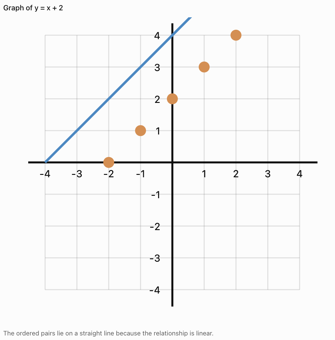
Graph the relationship:

y = x + 2

Step 1: Create a Table

Step 2: Write the Ordered Pairs

(−2, 0)

(−1, 1)

(0, 2)

(1, 3)

(2, 4)

Step 3: Plot the Points

Step 4: Interpret the Graph

As x increases by 1, y also increases by 1.

The graph is a straight line.

Important Observation

A table and a graph are two different representations of the same mathematical relationship.

Recognising Trends in Tables

A trend is a general pattern or direction in data.

Common trends include:

• Increasing

• Decreasing

• Constant

• Fluctuating

Increasing Trend

Distance increases as time increases.

Decreasing Trend

The amount of water decreases over time.

Constant Trend

The temperature remains unchanged.

Fluctuating Trend

The temperature rises and falls.

Important Observation

Identifying trends helps us describe how quantities change and make reasonable predictions.

Identifying Constant Differences

A table may show a pattern where the dependent variable changes by the same amount for every equal increase in the independent variable.

Example

The y-values increase by 3 each time x increases by 1.

Differences:

7 − 4 = 3

10 − 7 = 3

13 − 10 = 3

16 − 13 = 3

This is a linear relationship.

The rule is:

y = 3x + 1

Important Observation

A constant rate of change produces a straight-line graph.

Identifying Nonlinear Patterns

Not all relationships have constant differences.

Example

Consider:

y = x²

First differences:

1, 3, 5, 7

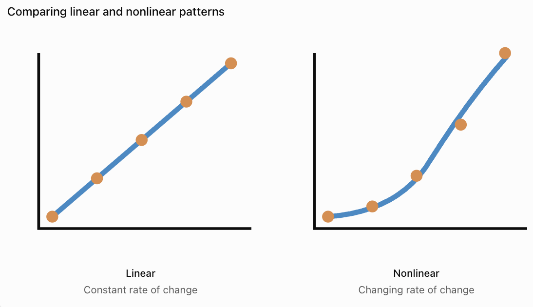
The differences are not constant.

However, the second differences are constant:

2, 2, 2

This is characteristic of a quadratic relationship when x-values are equally spaced.

Important Observation

Nonlinear relationships often produce curved graphs, although some nonlinear data may also produce other shapes.

Choosing the Correct Type of Graph

Different graphs are useful for different kinds of data.

Line Graphs

Line graphs are useful for showing changes in continuous quantities, especially over time.

Examples:

• Temperature over time.

• Distance travelled.

• Population growth.

• Water level changes.

Bar Graphs

Bar graphs are useful for comparing separate categories.

Examples:

• Favourite school subjects.

• Number of students in clubs.

• Sales of different products.

• Types of transportation used.

Scatter Plots

Scatter plots are useful for examining relationships between two numerical variables.

Examples:

• Height and mass.

• Study time and test scores.

• Temperature and reaction rate.

• Age and reaction time.

Important Observation

The best graph depends on the type of data and the relationship being investigated.

Creating a Line Graph from a Table

Worked Example: Plant Growth

A plant grows over five weeks.

Step 1: Identify the Variables

Independent variable: Week

Dependent variable: Plant height

Step 2: Label the Axes

x-axis: Week

y-axis: Height (cm)

Step 3: Choose a Scale

The x-axis should include weeks 0–4.

The y-axis should include heights from 0 to at least 16 cm.

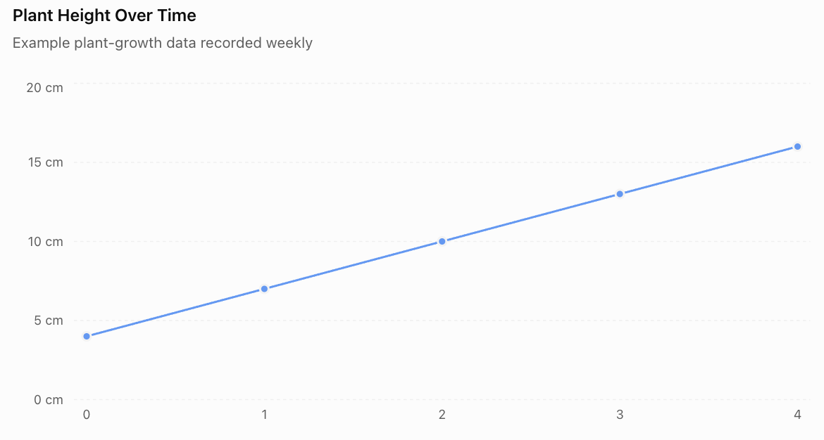
Step 4: Plot the Points

(0, 4)

(1, 7)

(2, 10)

(3, 13)

(4, 16)

Step 5: Connect the Points

Because the data describes a quantity changing over time, a line graph can be appropriate.

Step 6: Interpret the Graph

The plant grows by 3 cm each week.

The relationship is linear over the measured period.

Important Observation

The graph allows us to recognise the growth pattern more quickly than the table alone.

Interpreting Information from Graphs

Graphs provide information about quantities and their relationships.

When interpreting a graph, consider:

• What does the title describe?

• What does each axis represent?

• What units are used?

• What is the scale?

• Does the graph increase, decrease, or remain constant?

• Are there unusual values?

• What conclusions can be drawn?

Example

A graph shows the temperature of water increasing from 20°C to 80°C over six minutes.

We can conclude that:

• The water temperature increased.

• The total increase was 60°C.

• The average rate of temperature increase was 10°C per minute.

Calculation

Average rate = Change in temperature / Change in time

Average rate = (80 − 20)/6

Average rate = 10°C/min

Important Observation

Graphs allow us to calculate changes and rates of change.

Reading Values Between Data Points

Sometimes we need to estimate values that were not recorded directly.

This is called interpolation.

Example

A table shows:

If the temperature changes steadily, we can estimate the temperature at 3 minutes.

Between 2 and 4 minutes, the temperature increases from 30°C to 40°C.

At 3 minutes, the estimated temperature is:

35°C

Important Observation

Interpolation estimates values within the range of observed data.

It is generally more reliable when the relationship is regular and the data is consistent.

Predicting Values Beyond the Data

Estimating values outside the recorded range is called extrapolation.

Example

A plant grows at a steady rate of 3 cm per week.

Its height at week 4 is 16 cm.

Predict its height at week 6.

Two additional weeks of growth:

2 × 3 = 6 cm

Predicted height:

16 + 6 = 22 cm

Important Observation

Extrapolation assumes the observed pattern continues.

This assumption may not be valid over long periods.

For example, plants do not grow at a constant rate forever.

Comparing Tables and Graphs

Tables and graphs have different strengths.

Important Observation

Tables and graphs complement each other.

A table provides detailed numerical information, while a graph makes patterns easier to see.

Tables and Graphs in Science

Scientists frequently collect data in tables and represent results using graphs.

Example: Heating Water

A student heats water and records its temperature.

The table shows a constant increase of 9°C per minute.

A graph would show an upward-sloping straight line for these measurements.

Important Observation

Tables and graphs allow scientists to identify relationships between experimental variables.

Tables and Graphs in Everyday Life

Tables and graphs are also useful outside mathematics and science.

Examples

Personal Finance

A table can record monthly spending.

A graph can show changes in expenses over time.

Sports

A table can record scores.

A graph can show performance trends.

Weather

A table can record daily temperatures.

A graph can show changes throughout the week.

Education

A table can record test scores.

A graph can show improvement over time.

Transportation

A table can record journey times.

A graph can compare travel conditions.

Important Observation

Understanding tables and graphs helps us make informed decisions using evidence.

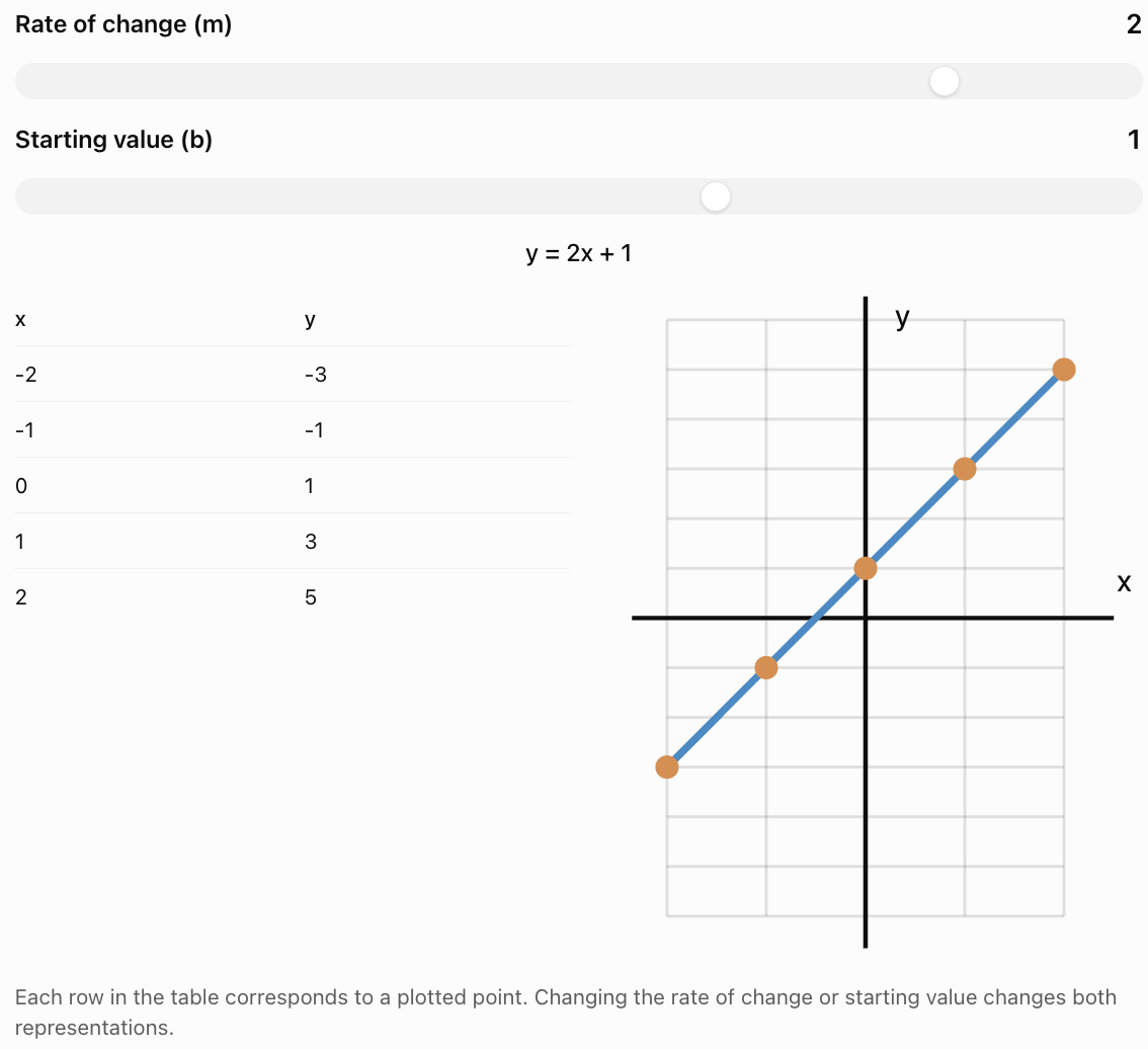
Interactive Table and Graph Explorer

Change the values in a linear relationship and observe how the table and graph change.

Common Mistakes

Forgetting table headings

Every column should clearly identify the information it contains.

Leaving out units

Measurements should include appropriate units.

Mixing up independent and dependent variables

The independent variable is usually placed in the first column and on the x-axis.

Reversing ordered pairs

Ordered pairs are written (x, y), not (y, x).

Using an inappropriate graph type

Bar graphs compare categories, while line graphs are often used for continuous changes.

Choosing an inconsistent scale

Axis intervals should increase consistently unless a clearly labelled scale break is used.

Plotting points inaccurately

Points should be placed at the correct coordinate locations.

Connecting unrelated categories with a line

Connecting categories can incorrectly suggest continuous values between them.

Assuming every pattern is linear

Some relationships are curved or irregular.

Making unsupported predictions

Extrapolation may not be reliable if the pattern changes.

Ignoring unusual data

Unexpected values may indicate errors or meaningful changes in the relationship.

Key Terms

• Data: Information collected through observations, measurements, or calculations.

• Data Table: Organised arrangement of information using rows and columns.

• Row: Horizontal arrangement of information in a table.

• Column: Vertical arrangement of information in a table.

• Heading: Label describing the information in a row or column.

• Variable: Quantity that can change.

• Independent Variable: Input quantity or variable deliberately changed.

• Dependent Variable: Output quantity that depends on another variable.

• Ordered Pair: Pair of coordinates written (x, y).

• Coordinate Plane: Grid used to locate points.

• Graph: Visual representation of data or mathematical relationships.

• Line Graph: Graph showing how a quantity changes, often over time.

• Bar Graph: Graph comparing categories using rectangular bars.

• Scatter Plot: Graph showing relationships between paired numerical values.

• Trend: General pattern or direction in data.

• Increasing Trend: Pattern in which values generally rise.

• Decreasing Trend: Pattern in which values generally fall.

• Constant Trend: Pattern in which values remain unchanged.

• Fluctuating Trend: Pattern in which values rise and fall.

• Linear Relationship: Relationship with a constant rate of change.

• Nonlinear Relationship: Relationship without a constant rate of change.

• Rate of Change: Amount one quantity changes relative to another.

• Scale: Numerical intervals used on a graph axis.

• Interpolation: Estimating values within the observed data range.

• Extrapolation: Estimating values outside the observed data range.

• Pattern: Regularity or relationship in a set of values.

• Prediction: Estimate based on observed information or a mathematical model.

Key Takeaways

• Tables organise data into rows and columns.

• Tables should include clear headings and appropriate units.

• Independent variables are commonly placed in the first column.

• Dependent variables are commonly placed in the second column.

• Tables can be created from patterns and equations.

• Each row of an x-y table can be written as an ordered pair.

• Ordered pairs can be plotted on a coordinate plane.

• Graphs make trends and relationships easier to recognise.

• Linear relationships have constant rates of change.

• Nonlinear relationships have changing rates of change.

• Line graphs are useful for showing continuous changes.

• Bar graphs are useful for comparing categories.

• Scatter plots help identify relationships between numerical variables.

• Tables provide exact values, while graphs show visual patterns.

• Interpolation estimates values within a data range.

• Extrapolation predicts values beyond the data range.

• Tables and graphs are important tools in mathematics, science, and everyday life.

Check Your Understanding

Understanding Tables

1. What is a data table?

2. What is the difference between a row and a column?

3. Why should tables include headings?

4. Why are units important in data tables?

5. Explain the difference between an independent and dependent variable.

Creating Tables

6. Create a table for the pattern 2, 4, 6, 8, 10.

7. Create a table of values for y = 3x when x = 0, 1, 2, 3, 4.

8. Create a table for y = x + 4 when x = −2, −1, 0, 1, 2.

9. Convert the table from Question 8 into ordered pairs.

10. Explain how a table can be used to generate points for a graph.

Identifying Trends

11. A table shows values 5, 10, 15, 20, 25. Describe the trend.

12. A table shows values 30, 25, 20, 15, 10. Describe the trend.

13. A table shows values 12, 12, 12, 12. Describe the trend.

14. A table shows values 4, 7, 5, 9, 6. Describe the trend.

15. Explain how you can recognise a linear relationship from a table with equally spaced x-values.

Interpreting Graphs

16. What type of graph is useful for showing temperature changes over time?

17. What type of graph is useful for comparing favourite school subjects?

18. A graph shows distance increasing from 0 m to 100 m in 20 seconds. Calculate the average speed.

19. Explain the difference between interpolation and extrapolation.

20. Describe one advantage of a graph compared with a table.

Answer Key

Extended Challenge

1. Complete the table for y = 2x + 3 when x = −3, −2, −1, 0, 1, 2, 3.

2. A table contains the values x = 1, 2, 3, 4 and y = 5, 8, 11, 14. Determine the equation relating x and y.

3. A plant grows from 6 cm to 21 cm over five weeks. Calculate its average growth rate.

4. A car travels at a constant speed of 12 m/s. Create a table showing the distance travelled at 0, 1, 2, 3, 4, and 5 seconds.

5. A table shows x-values 0, 1, 2, 3, 4 and y-values 1, 4, 9, 16, 25. Determine a rule for the relationship.

6. A student records temperatures of 18°C, 22°C, 26°C, 30°C, and 34°C at equal time intervals. Describe the trend and calculate the increase between measurements.

7. Explain why a bar graph is more appropriate than a line graph for comparing the number of students in different clubs.

8. A table shows a constant increase of 7 units in y for every increase of 2 units in x. Determine the rate of change.

9. A graph shows that a water tank contains 120 L at 0 minutes and 60 L at 10 minutes. Calculate the average rate of change.

10. Explain why extrapolating a plant's growth rate over several years may be unreliable.

Extended Challenge Answers

Final Investigation: Investigating a Mathematical Relationship

A student is investigating the relationship between time and distance travelled by a toy car moving at a constant speed.

The student records the following data:

Part A: Organising the Data

1. Identify the independent variable.

2. Identify the dependent variable.

3. Explain why the table is organised in this order.

4. Determine the increase in distance for each one-second interval.

5. Describe the trend shown in the table.

Part B: Creating a Graph

6. Draw a coordinate plane.

7. Label the x-axis as Time (s).

8. Label the y-axis as Distance (cm).

9. Choose appropriate scales.

10. Plot all six ordered pairs.

11. Connect the points appropriately.

12. Describe the shape of the graph.

Part C: Analysing the Relationship

13. Calculate the average speed of the toy car.

14. Write an equation relating distance and time.

15. Use the equation to predict the distance travelled after 7 seconds.

16. Estimate the distance travelled after 2.5 seconds.

17. Explain why the graph passes through the origin.

Part D: Evaluating the Data

18. Explain why a line graph is appropriate.

19. Describe one possible source of experimental error.

20. Explain how the student could improve the reliability of the investigation.

Investigation Answer Check

Variables

• Independent variable: Time

• Dependent variable: Distance

Trend

Distance increases by 15 cm each second.

Graph

The points form a straight line passing through the origin.

Average Speed

Speed = Distance / Time

Speed = 75/5

Speed = 15 cm/s

Equation

d = 15t

where d is distance in centimetres and t is time in seconds.

Prediction at 7 Seconds

d = 15 × 7

d = 105 cm

Interpolation at 2.5 Seconds

d = 15 × 2.5

d = 37.5 cm

Reliability

Repeating the investigation, using consistent measuring techniques, and averaging repeated measurements can improve reliability.

Final Reflection

Tables and graphs are essential tools for organising and interpreting information.

Tables allow us to record exact values and identify numerical patterns. Graphs make relationships and trends easier to recognise.

By learning to create tables, generate ordered pairs, plot graphs, and interpret data, we develop important mathematical skills that can be applied throughout science, technology, engineering, and everyday life.