1. Making Predictions from Data

Learning outcomes
  • I can identify trends and patterns in data.
  • I can use data to make predictions.
  • I can evaluate the reliability of predictions.
  • I can explain limitations of forecasting.
  • I can justify predictions using evidence from data.

Making Predictions from Data

Data can help us understand what has happened in the past and make informed predictions about what might happen in the future.

A prediction is an estimate of an unknown or future value based on available information.

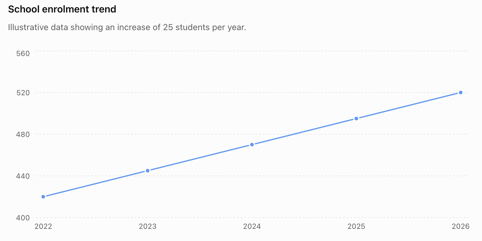
For example, suppose a school's enrolment has been:

Year Students
2022 420
2023 445
2024 470
2025 495
2026 520

The number of students has increased by approximately 25 each year. If this pattern continues, we might predict:

2027 enrolment ≈ 545 students

This prediction is supported by the observed trend. However, it is still a prediction—not a guarantee.
Identifying Trends

A trend is the general direction in which data change.

Three common trends are:

Increasing trend — values generally increase.

Decreasing trend — values generally decrease.

No clear trend — values fluctuate without a consistent overall direction.

For example:

12, 15, 19, 22, 26

shows an increasing trend.

80, 73, 69, 61, 55

shows a decreasing trend.

20, 35, 18, 32, 21

does not show a simple consistent trend.

Trends Do Not Need to Be Perfect

Real data rarely follow a perfectly smooth pattern.

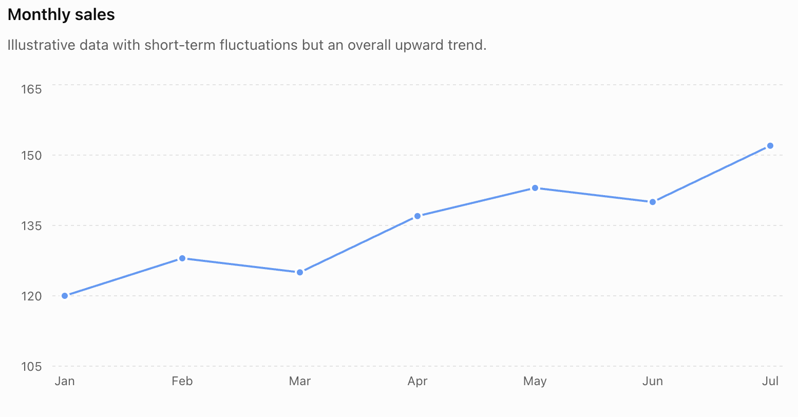
Consider:

Month Sales
January 120
February 128
March 125
April 137
May 143
June 140
July 152

Sales occasionally decrease, but the overall trend is upward.

We should therefore distinguish between short-term fluctuations and the broader pattern.
Patterns in Data

A pattern is a recognizable structure or regularity in data.

Patterns can include:

  • constant increases or decreases
  • repeating cycles
  • seasonal changes
  • proportional relationships
  • accelerating growth
  • slowing growth
  • clusters
  • unusual values
  • relationships between variables

Recognizing the type of pattern helps us decide how predictions should be made.

Constant Change

Consider:

5, 8, 11, 14, 17

The difference between consecutive values is always:

+3

If the pattern continues, the next value would be:

20

This is a linear pattern because the change is constant.

Percentage Growth

Some quantities increase by a percentage rather than by a constant amount.

Suppose a population increases by 5% each year.

If the current population is 20,000:

Next year:

20,000 × 1.05 = 21,000

The following year:

21,000 × 1.05 = 22,050

The amount added becomes larger each year.

This produces an exponential pattern rather than a linear one.

Cyclical and Seasonal Patterns

Some patterns repeat.

For example, electricity consumption might rise every summer because of air-conditioning use and then fall during cooler months.

Retail sales may rise each December and fall in January.

This is a seasonal pattern.

If we ignored the seasonal cycle and simply extended a short-term increase, our prediction could be misleading.

Scatter Plots and Relationships

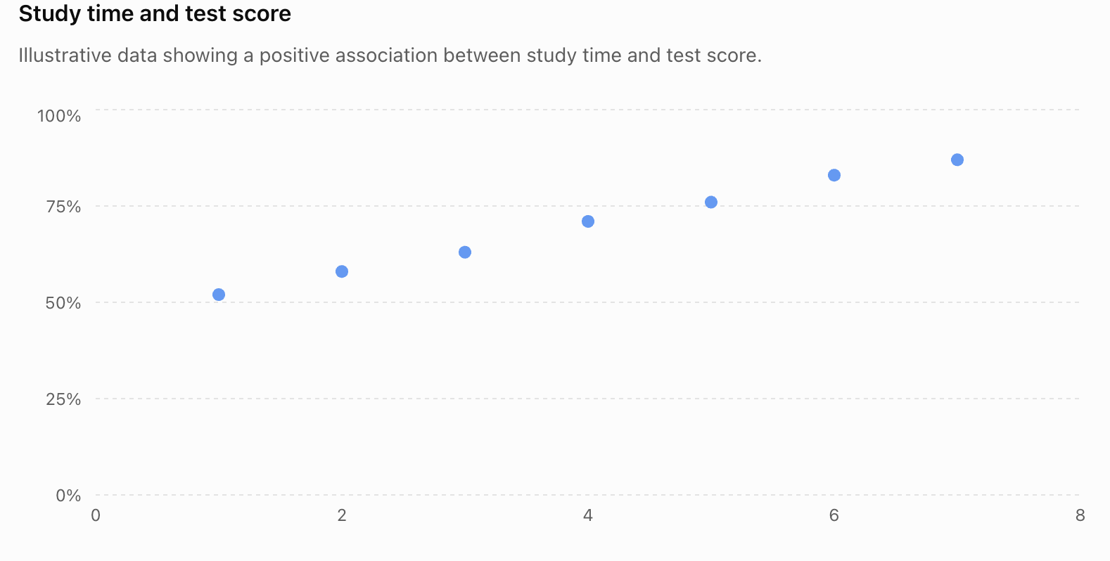
When data involve two numerical variables, a scatter plot can help reveal whether they are related.

For example, consider hours studied and test scores.

Hours Studied Test Score (%)
1 52
2 58
3 63
4 71
5 76
6 83
7 87

As study time increases, test scores also tend to increase.

This is called a positive association or positive correlation.

Positive and Negative Correlation

A positive correlation occurs when one variable tends to increase as the other increases.

Examples might include:

  • height and arm span
  • study time and test performance
  • advertising expenditure and sales

A negative correlation occurs when one variable tends to decrease as the other increases.

Examples might include:

  • speed and travel time for a fixed distance
  • outside temperature and heating use

If there is no obvious relationship, the variables may have little or no correlation.

Correlation Does Not Prove Causation

Suppose two variables are strongly correlated.

This does not automatically mean that one variable causes the other.

For example, ice-cream sales and sunburn cases may both increase during hot weather.

It would be incorrect to conclude:

Buying ice cream causes sunburn.

A third variable—temperature or sunny weather—helps explain why both increase.

Therefore:

correlation does not necessarily imply causation.

Making Predictions from a Trend

Suppose a plant's measured height is:

Week Height (cm)
1 8
2 11
3 14
4 17
5 20

The plant has grown approximately:

3 cm per week

A reasonable prediction for Week 6 would be:

20 + 3 = 23 cm

For Week 7:

23 + 3 = 26 cm

These predictions assume the existing growth pattern continues.

Using a Simple Linear Model

A linear relationship can often be represented as:

y = mx + b

where:

  • m = rate of change or slope
  • b = starting value
  • x = independent variable
  • y = predicted value

Suppose a company's sales can approximately be modeled by:

S = 200 + 15t

where S represents sales and t represents months.

For t = 6:

S = 200 + 15(6)

= 200 + 90

= 290

The model predicts approximately 290 sales after six months.

Predictions Are Estimates

A model such as:

S = 200 + 15t

does not mean sales must equal exactly 290.

Real data may be affected by:

  • customer behaviour
  • economic changes
  • competition
  • weather
  • advertising
  • supply problems
  • random variation

A prediction should therefore usually be described as an estimate.

Interpolation

Interpolation means predicting a value within the range of observed data.

Suppose:

Time Temperature
10:00 20°C
12:00 24°C

We want to estimate the temperature at 11:00.

Since 11:00 lies between the measured times, this is interpolation.

If we assume approximately linear change:

temperature ≈ 22°C

Interpolation is often relatively reliable because the prediction lies between known data points.

Extrapolation

Extrapolation means predicting a value outside the range of observed data.

Using the same data, predicting the temperature at 18:00 would be extrapolation.

The prediction is less certain because conditions may change after the measured period.

For example:

  • clouds may arrive
  • the Sun may begin setting
  • rain may occur
  • wind conditions may change

The farther we extrapolate beyond the observed data, the more cautious we should generally be.

Interpolation Versus Extrapolation

Method Prediction location General reliability
Interpolation Inside observed range Usually more reliable
Extrapolation Outside observed range Usually less reliable

This does not mean interpolation is always correct or extrapolation is always poor. It means extrapolation usually requires stronger assumptions about whether the pattern will continue.

Lines of Best Fit

Scatter plots often contain points that do not fall exactly on a straight line.

A line of best fit represents the overall linear trend.

The line does not need to pass through every point.

Instead, it should represent the general relationship between the variables.

A line of best fit can then be used to estimate values.

For example, if a line of best fit suggests:

y = 5x + 40

then for x = 6:

y = 5(6) + 40

= 70

So the predicted value is approximately 70.

Residuals

A residual measures the difference between an observed value and the value predicted by a model.

A common convention is:

residual = observed value − predicted value

Suppose a model predicts:

72

but the observed value is:

76

Then:

residual = 76 − 72

= 4

A small residual indicates that the prediction was close to the observed value.

Large residuals may indicate that:

  • the model does not fit well
  • the data contain unusual observations
  • important variables are missing
  • a different type of model may be needed

Outliers

An outlier is a data value that is unusually far from the general pattern.

Suppose most test scores are:

72, 75, 78, 80, 81, 84, 85

but one score is:

25

The score of 25 may be an outlier.

Outliers can strongly affect:

  • averages
  • trend lines
  • correlation
  • predictions

However, an outlier should not automatically be deleted.

We should investigate why it occurred.

It could represent:

  • a measurement error
  • a recording error
  • an unusual but genuine event
  • an important change in the system

Reliability of Predictions

A prediction is reliable when we have good reason to expect it to be reasonably accurate.

Reliability depends on several factors.

Amount of Data

Predictions based on many observations are often more reliable than predictions based on only a few.

For example, predicting next year's rainfall from 30 years of measurements is generally more defensible than predicting it from only two years.

However, more data do not automatically guarantee a good prediction.

The data must also be relevant and of good quality.

Quality of Data

Predictions depend on the quality of the original measurements.

Poor-quality data may contain:

  • measurement errors
  • incorrect entries
  • missing observations
  • biased samples
  • inconsistent measurement methods

A sophisticated model cannot completely compensate for unreliable data.

Strength of the Pattern

A clear and consistent trend generally supports stronger predictions.

If points are tightly grouped around a trend, predictions may be more reliable.

If points are widely scattered, there is greater uncertainty.

Range of Prediction

Predictions close to the observed data are generally safer than predictions far beyond it.

Suppose we have data from 2020–2026.

Predicting 2027 requires only a small extrapolation.

Predicting 2075 assumes the same relationship continues for almost another 50 years.

That is a much stronger assumption.

Stability of the System

Prediction is easier when the system being studied is relatively stable.

For example, a machine operating under controlled conditions may produce highly predictable data.

Human behaviour, economic conditions, ecosystems, and weather can be much more complicated.

A previously observed trend can change.

Sample Size

A sample is the group from which data are collected.

Suppose we ask 5 students which school lunch they prefer and use their answers to predict the preferences of 2,000 students.

The sample is probably too small to support a strong prediction.

A larger, representative sample would generally provide better evidence.

Representative Samples

Sample size alone is not enough.

Suppose a school wants to predict whether students support a later school start time.

Surveying 500 students sounds impressive.

But if all 500 are Grade 12 students, the sample may not represent the entire school.

A good sample should reflect the population about which the prediction is being made.

Bias

Bias is a systematic influence that pushes data or conclusions in a particular direction.

Bias may arise from:

  • how participants are selected
  • how questions are worded
  • which data are included
  • measurement techniques
  • non-response
  • researchers' choices

Biased data can produce misleading predictions even when the calculations are mathematically correct.

Forecasting

A forecast is a prediction about a future quantity, usually based on past and current data.

Forecasts are common in:

  • weather
  • economics
  • population studies
  • business
  • transportation
  • energy use
  • public health
  • sports

Forecasting usually involves assumptions about how past relationships will behave in the future.

Why Forecasts Can Fail

Forecasts can fail when circumstances change.

Suppose a restaurant's customers increase steadily:

100, 110, 120, 130, 140 per day.

A simple trend predicts:

150 customers next

But several events could disrupt the trend:

  • a competitor opens nearby
  • prices increase
  • the restaurant closes temporarily
  • a holiday changes customer behaviour
  • transportation access changes

The mathematical pattern does not know about these events unless they are included in the model.

Models Are Simplifications

A mathematical model represents some features of a real system.

It cannot normally include every factor.

For example, a model predicting crop yield might include:

  • rainfall
  • temperature
  • fertilizer use

but perhaps not:

  • insect damage
  • soil variation
  • plant disease
  • unusual storms

Therefore, model predictions always have limitations.

Uncertainty

Good forecasting acknowledges uncertainty.

Instead of saying:

There will be exactly 1,250 customers next month.

a more appropriate statement might be:

Based on the recent trend, approximately 1,250 customers are expected next month, assuming current conditions continue.

This communicates both:

  • the prediction
  • the assumption behind it

Prediction Intervals

Sometimes uncertainty can be expressed as a range.

Instead of predicting:

500 units

a model might predict:

approximately 470–530 units

The range communicates that the exact future value is uncertain.

In more advanced statistics, a prediction interval is calculated using a formal statistical model to describe a range of plausible future observations.

Comparing Predictions

Suppose two students make predictions from this sequence:

20, 24, 28, 32, 36

Student A predicts:

40

Student B predicts:

60

Student A has stronger evidence.

The data increase consistently by:

+4

Therefore:

36 + 4 = 40

Student B may still turn out to be correct by chance, but the available data do not strongly support that prediction.

A good prediction is judged by its reasoning and evidence, not merely by whether it happens to come true.

Justifying a Prediction

A strong justification should identify:

  • the observed trend or pattern
  • relevant numerical evidence
  • the prediction
  • the method used
  • important assumptions
  • sources of uncertainty

For example:

The number of visitors increased from 1,200 to 1,500 over three months, an average increase of about 100 visitors per month. If this approximately linear trend continues, I would predict about 1,600 visitors next month. However, the estimate may be unreliable if visitor numbers are strongly seasonal.

This is much stronger than simply saying:

I predict 1,600.

Comparing Models

Different models may produce different predictions from the same data.

For example, one model might assume:

constant increase

while another assumes:

constant percentage growth

Suppose a quantity changes:

100 → 120 → 144

The increase is:

+20, then +24

so the increase is not constant.

But each value is:

1.2 times the previous value

This suggests approximately:

20% growth per period

A percentage-growth model may therefore be more appropriate than a linear model.

The next predicted value would be:

144 × 1.2

= 172.8

Avoiding Unjustified Precision

Suppose a rough graph suggests next year's population will be around:

52,000

Reporting:

51,987.436 people

would imply a level of precision that the data do not support.

Predictions should reflect the precision and uncertainty of the evidence.

Appropriate:

approximately 52,000

Potentially misleading:

51,987.436

This idea is sometimes called avoiding false precision.

Comparing Forecast with Actual Results

When the actual result becomes available, it can be compared with the prediction.

One simple measure is:

prediction error = actual value − predicted value

Suppose:

predicted sales = 850
actual sales = 810

Then:

prediction error = 810 − 850

= −40

The negative result means the prediction was 40 units too high.

The absolute error is:

|−40| = 40

Percentage Error

When comparing predictions across different scales, percentage error can be useful.

percentage error = |actual − predicted| / |actual| × 100%

Suppose:

actual = 200
predicted = 190

Then:

percentage error = |200 − 190| / 200 × 100%

= 10/200 × 100%

= 5%

A smaller percentage error generally indicates a closer prediction.

Improving Predictions

Predictions can often be improved by:

  • collecting more data
  • improving measurement accuracy
  • using representative samples
  • identifying outliers
  • considering seasonal patterns
  • including important variables
  • choosing a model appropriate to the pattern
  • reducing the amount of extrapolation
  • updating models when new data become available

Forecasting is often an ongoing process rather than a single calculation.

Authentic Example: School Cafeteria Demand

Suppose the number of lunches sold during five Mondays is:

Monday Lunches Sold
1 410
2 425
3 438
4 452
5 467

The increases are:

+15, +13, +14, +15

The pattern suggests an increase of approximately:

14 lunches per week

A reasonable prediction for Monday 6 would therefore be:

467 + 14 = 481 lunches

A useful conclusion would be:

Based on the previous five Mondays, lunch sales have increased by about 14 meals per week. If this trend continues, approximately 480 lunches may be needed next Monday.

This prediction is evidence-based but still acknowledges uncertainty.

Limitations of the Cafeteria Prediction

The prediction might fail because:

  • student attendance changes
  • the menu changes
  • there is a school event
  • prices change
  • the weather affects attendance
  • the observed trend does not continue

Therefore, a prediction should not be treated as certainty.

A Strategy for Making Predictions

When given a data set:

Examine the data.

Look for increases, decreases, cycles, clusters, and unusual values.

Describe the pattern.

For example:

"The values increase by approximately 5 each month."

Choose an appropriate model or method.

This might involve:

  • extending a pattern
  • calculating an average rate of change
  • using a line of best fit
  • applying percentage growth
  • accounting for seasonal behaviour

Calculate the prediction.

Show enough working that the reasoning can be checked.

Evaluate reliability.

Consider the amount, quality, and consistency of the data.

State limitations.

Identify assumptions and factors that could cause the prediction to fail.

Give a justified conclusion.

Use language such as:

approximately

the data suggest

if the current trend continues

based on the available evidence

Common Mistakes

Assuming a trend must continue forever

Real systems change. Long-range extrapolation can be especially unreliable.

Ignoring fluctuations

A general trend does not mean every observation follows it exactly.

Using too few data points

Two observations may not be enough to establish a meaningful trend.

Ignoring outliers

An unusual value may affect the model and should be investigated.

Automatically deleting outliers

An outlier may contain important information rather than being an error.

Confusing correlation with causation

Two variables changing together does not prove that one causes the other.

Ignoring the domain of the data

A model that works within the observed range may behave unrealistically outside it.

Using an inappropriate model

Linear growth should not automatically be assumed when the data show exponential or seasonal behaviour.

Giving predictions with excessive precision

The precision of a prediction should reflect the quality of the evidence.

Making a prediction without justification

A numerical answer should be supported by the pattern or model used.

Key Terms

Data — collected observations or measurements used for analysis.

Trend — the overall direction in which data are changing.

Pattern — a recognizable regularity or structure in data.

Prediction — an estimate of an unknown or future value based on available evidence.

Forecast — a prediction of a future quantity based on data and a model or observed pattern.

Interpolation — estimating a value within the range of observed data.

Extrapolation — estimating a value outside the range of observed data.

Correlation — a statistical relationship between variables.

Positive correlation — a relationship in which larger values of one variable tend to occur with larger values of another.

Negative correlation — a relationship in which larger values of one variable tend to occur with smaller values of another.

Line of best fit — a line used to represent the overall linear trend in data.

Model — a mathematical representation used to describe or predict a system.

Residual — the difference between an observed value and its predicted value.

Outlier — a value unusually far from the overall pattern.

Bias — a systematic influence that can distort data or conclusions.

Sample — a subset of a population from which information is collected.

Representative sample — a sample that reasonably reflects the population being studied.

Prediction error — the difference between an observed result and its predicted value.

Uncertainty — the degree to which the exact outcome of a prediction is unknown.

Key Takeaways

  • Data can reveal trends and patterns that can be used to make predictions.
  • Trends may be increasing, decreasing, cyclical, seasonal, linear, or non-linear.
  • Real data usually contain variation, so trends do not need to be perfectly smooth.
  • Interpolation predicts within the observed data range.
  • Extrapolation predicts beyond the observed range and is generally more uncertain.
  • Scatter plots and lines of best fit can help identify relationships between variables.
  • Correlation does not necessarily imply causation.
  • Prediction reliability depends on data quantity, quality, consistency, sampling, and the strength of the pattern.
  • Outliers should be investigated rather than automatically ignored.
  • Models simplify reality and cannot normally account for every factor.
  • Long-range forecasts usually involve greater uncertainty.
  • Predictions should not imply more precision than the evidence supports.
  • Strong predictions identify the pattern, use numerical evidence, explain the method, and acknowledge limitations.
  • Predictions should be updated when new evidence becomes available.
  • A prediction is an evidence-based estimate, not a guarantee.

Check Your Understanding

  1. Describe the trend in the data:

    12, 17, 22, 27, 32

    Predict the next value and justify your answer.

  2. Consider:

    100, 90, 81, 73, 66

    Is a constant decrease or percentage decrease likely to describe the pattern better? Explain.

  3. A plant grows from 12 cm in Week 1 to 15 cm, 18 cm, 21 cm, and 24 cm in the following weeks. Predict its height in Week 6 if the pattern continues.
  4. Explain the difference between interpolation and extrapolation.
  5. Temperature is measured at 10:00, 12:00, 14:00, and 16:00. Would estimating the temperature at 13:00 involve interpolation or extrapolation?
  6. Using the same data, would predicting the temperature at 22:00 involve interpolation or extrapolation? Explain why this prediction might be less reliable.
  7. A line of best fit is:

    y = 4x + 15

    Use the model to predict y when x = 12.

  8. A model predicts a value of 72, while the observed value is 78. Calculate the residual using:

    residual = observed − predicted

  9. A company predicts sales of 950 units but actually sells 1,000 units. Calculate the percentage error.
  10. Explain why a prediction based on 20 years of relevant data may be more reliable than one based on two observations.
  11. A scatter plot shows that students who sleep longer tend to achieve higher test scores. Explain why this does not, by itself, prove that additional sleep causes higher scores.
  12. A data set follows a clear increasing trend except for one unusually low value. Explain what should be considered before deciding whether to remove the outlier.
  13. A town's population increased by about 500 people per year from 2022 to 2026. Explain why extending this trend to predict the population in 2027 may be more reliable than using it to predict the population in 2075.
  14. Two students predict next month's sales. Student A predicts 420 units and explains that sales have increased by approximately 20 units per month for the previous six months. Student B predicts 600 units but provides no model or supporting evidence. Which prediction is better justified, and why?
  15. A forecast states:

"Based on the current trend, approximately 8,000 visitors are expected next month, assuming seasonal conditions remain similar."

Explain why this is a stronger mathematical statement than:

"Exactly 8,000 visitors will come next month."