1. Making Predictions from Data

Making Predictions from Data

Data can help us understand what has happened in the past and make informed predictions about what might happen in the future.

A prediction is an estimate of an unknown or future value based on available information.

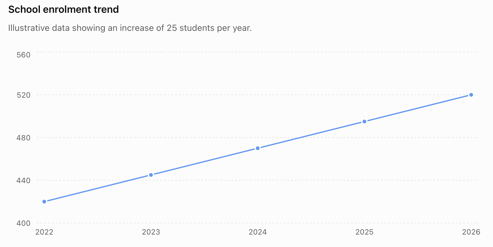
For example, suppose a school's enrolment has been:

The number of students has increased by approximately 25 each year. If this pattern continues, we might predict:

2027 enrolment ≈ 545 students

This prediction is supported by the observed trend. However, it is still a prediction—not a guarantee.

Identifying Trends

A trend is the general direction in which data change.

Three common trends are:

Increasing trend — values generally increase.

Decreasing trend — values generally decrease.

No clear trend — values fluctuate without a consistent overall direction.

For example:

12, 15, 19, 22, 26

shows an increasing trend.

80, 73, 69, 61, 55

shows a decreasing trend.

20, 35, 18, 32, 21

does not show a simple consistent trend.

Trends Do Not Need to Be Perfect

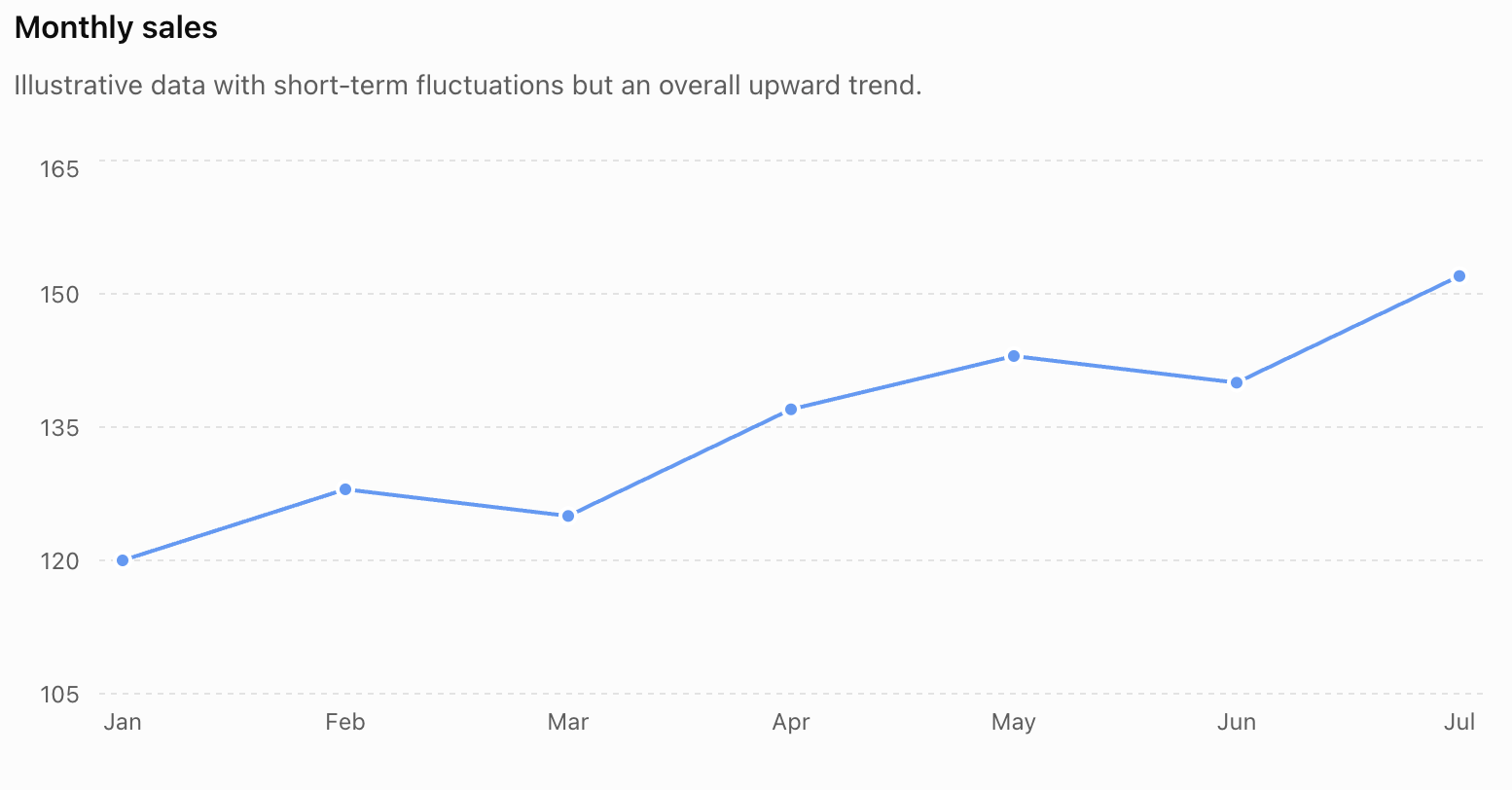
Real data rarely follow a perfectly smooth pattern.

Consider:

Sales occasionally decrease, but the overall trend is upward.

We should therefore distinguish between short-term fluctuations and the broader pattern.

Patterns in Data

A pattern is a recognizable structure or regularity in data.

Patterns can include:

• constant increases or decreases
• repeating cycles
• seasonal changes
• proportional relationships
• accelerating growth
• slowing growth
• clusters
• unusual values
• relationships between variables

Recognizing the type of pattern helps us decide how predictions should be made.

Constant Change

Consider:

5, 8, 11, 14, 17

The difference between consecutive values is always:

+3

If the pattern continues, the next value would be:

20

This is a linear pattern because the change is constant.

Percentage Growth

Some quantities increase by a percentage rather than by a constant amount.

Suppose a population increases by 5% each year.

If the current population is 20,000:

Next year:

20,000 × 1.05 = 21,000

The following year:

21,000 × 1.05 = 22,050

The amount added becomes larger each year.

This produces an exponential pattern rather than a linear one.

Cyclical and Seasonal Patterns

Some patterns repeat.

For example, electricity consumption might rise every summer because of air-conditioning use and then fall during cooler months.

Retail sales may rise each December and fall in January.

This is a seasonal pattern.

If we ignored the seasonal cycle and simply extended a short-term increase, our prediction could be misleading.

Scatter Plots and Relationships

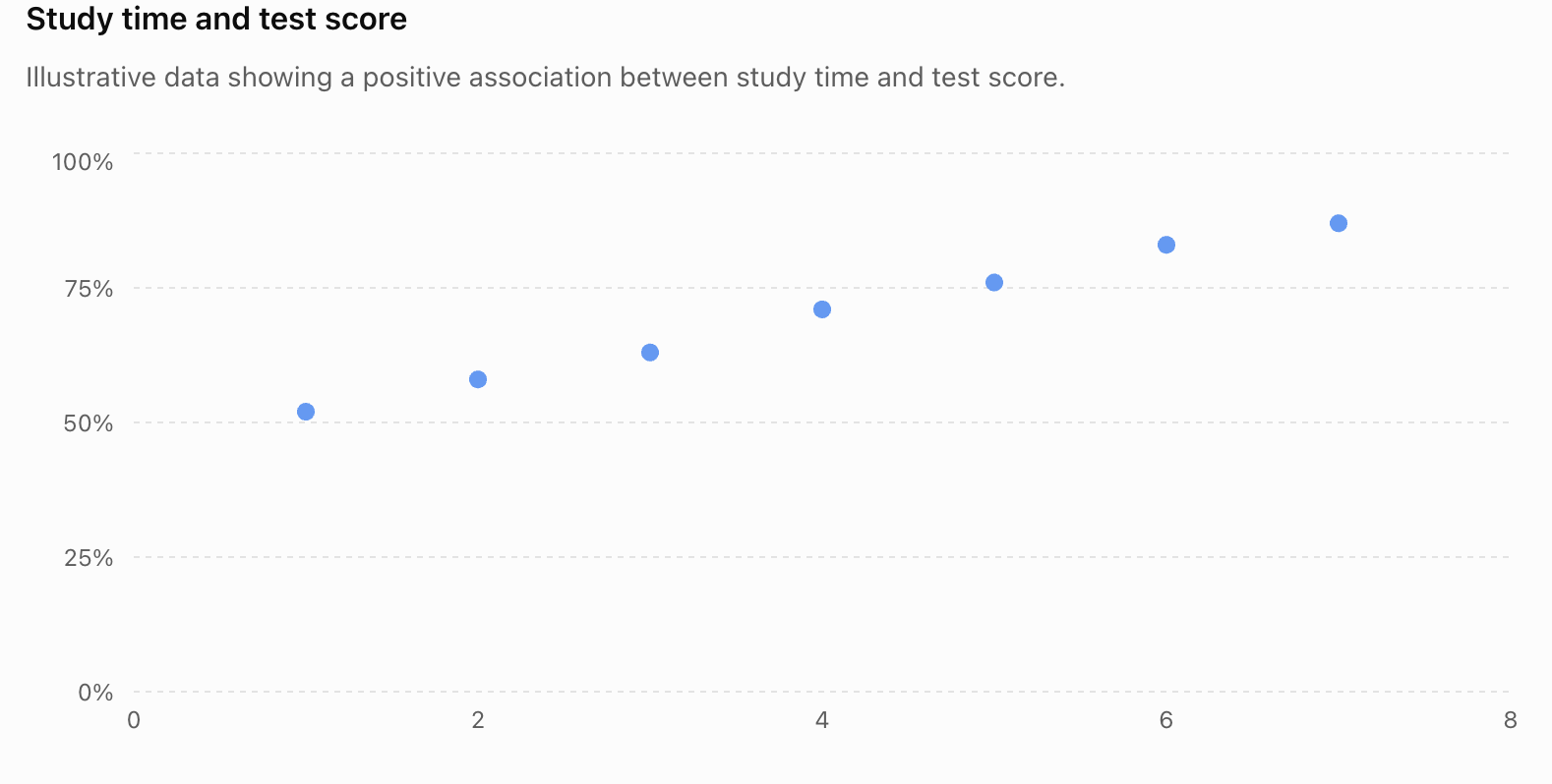
When data involve two numerical variables, a scatter plot can help reveal whether they are related.

For example, consider hours studied and test scores.

2. Probability and Fairness

Probability and Fairness

Probability provides a mathematical way to decide whether a game, competition, or random activity is fair.

In a simple two-player chance game, we often call the game fair when both players have the same probability of winning. More generally, when prizes, costs, or different outcomes are involved, fairness can be analysed using expected value: neither side should have a long-term mathematical advantage if the game is financially fair.

For example, suppose two players toss a fair coin.

• Player A wins if the coin lands heads.
• Player B wins if the coin lands tails.

Since:

P(heads) = 1/2

and:

P(tails) = 1/2

each player has the same probability of winning.

Therefore, the game is fair.

Probability and Fairness

For equally likely outcomes:

P(event) = number of favourable outcomes / total number of possible outcomes

A probability is always between:

0 and 1

where:

P(event) = 0 means impossible.

P(event) = 1 means certain.

For a fair six-sided die:

P(1) = P(2) = P(3) = P(4) = P(5) = P(6) = 1/6

 

 

Equal probabilities of individual outcomes do not automatically mean that every game using the die is fair. The rules determine which outcomes cause each player to win.

A Simple Fair Dice Game

Suppose:

• Player A wins if an odd number is rolled.
• Player B wins if an even number is rolled.

The possible outcomes are:

{1, 2, 3, 4, 5, 6}

Player A wins with:

{1, 3, 5}

Therefore:

P(A wins) = 3/6 = 1/2

Player B wins with:

{2, 4, 6}

Therefore:

P(B wins) = 3/6 = 1/2

Both players have equal probabilities of winning.

Therefore:

the game is fair.

An Unfair Dice Game

Now change the rules:

• Player A wins by rolling 1, 2, 3, or 4.
• Player B wins by rolling 5 or 6.

Then:

P(A wins) = 4/6 = 2/3

and:

P(B wins) = 2/6 = 1/3

Player A is twice as likely to win.

Therefore:

the game is unfair.

Notice that the die itself is still fair. It is the rules of the game that create the unfairness.

Fair Random Devices

A random device is fair when its intended basic outcomes are equally likely.

Examples include:

• a balanced coin
• a properly constructed six-sided die
• a spinner divided into equal sections
• well-shuffled identical cards

For a spinner divided into four equal sections:

P(each section) = 1/4 = 25%

 

 

If the sections are unequal in size, their probabilities will generally not be equal.

That does not necessarily make a game unfair, however. The rules and rewards could compensate for the unequal probabilities.

Fairness Is About the Whole Game

Consider a spinner with:

• red probability = 1/2
• blue probability = 1/4
• green probability = 1/4

If:

• Player A wins on red
• Player B wins on blue or green

then:

P(A wins) = 1/2

and:

P(B wins) = 1/4 + 1/4 = 1/2

The spinner has unequal colour probabilities, but the game is fair between the two players.

This illustrates an important principle:

Fairness depends on the probabilities created by the complete rules, not simply on whether every individual outcome is equally likely.

Theoretical Probability

Theoretical probability is calculated from the mathematical structure of an experiment.

For a fair die:

P(rolling a 6) = 1/6

This probability does not mean that exactly one of every six rolls must be a 6.

It describes what we expect over many trials.

Experimental Probability

Experimental probability is calculated from actual results:

experimental probability = number of times event occurs / total number of trials

Suppose a die is rolled 60 times and 6 appears 13 times.

Then:

experimental P(6) = 13/60 ≈ 0.217

The theoretical probability is:

P(6) = 1/6 ≈ 0.167

These values are different.

That does not automatically mean the die is unfair.

Random variation is expected, especially with relatively small numbers of trials.

Short-Term Results Can Look Unfair

Suppose two people play a perfectly fair coin-toss game ten times.

Player A might win seven games.

Player B might win three.

That result does not prove that the game was unfair.

Fairness means that both players had equal probabilities before each game—not that they must win exactly the same number of times.

As the number of trials becomes very large, experimental proportions often tend to move closer to their theoretical probabilities. This is connected to the law of large numbers.

Expected Outcomes

Probability can be used to calculate how many times we expect an event to occur.

The basic relationship is:

expected frequency = probability × number of trials

Suppose a fair die is rolled 600 times.

The probability of rolling a 6 is:

1/6

Therefore:

expected number of 6s = 1/6 × 600

= 100

We expect approximately 100 sixes.

This does not mean there must be exactly 100.

Expected Outcome Example

A coin is tossed 200 times.

What is the expected number of heads?

P(heads) = 1/2

Therefore:

expected heads = 1/2 × 200

= 100

We would expect approximately 100 heads.

Results such as 96 heads or 107 heads would not be surprising.

Two-Stage Expected Outcomes

Suppose two fair coins are tossed.

The possible equally likely outcomes are:

HH, HT, TH, TT

There are four possibilities.

The probability of two heads is:

P(HH) = 1/4

If the experiment is repeated 200 times:

expected HH outcomes = 1/4 × 200

= 50

So we expect approximately 50 cases of two heads.

 

 

 

5

Expected Value

When different outcomes have different numerical rewards, we can calculate expected value.

For outcomes x₁, x₂, x₃, ... with probabilities P₁, P₂, P₃, ...:

E(X) = x₁P₁ + x₂P₂ + x₃P₃ + ...

In simpler words:

expected value = sum of (outcome value × probability)

Expected value describes the average result we would expect per play in the long run.

Expected Value Example

Suppose a game works like this:

• win $6 with probability 1/4
• win $2 with probability 1/2
• win $0 with probability 1/4

The expected winnings are:

E(X) = 6(1/4) + 2(1/2) + 0(1/4)

= 1.50 + 1.00

= $2.50

Therefore, the average expected payout is:

$2.50 per game

If the game costs exactly $2.50 to play, its expected net value to the player is:

$2.50 − $2.50 = $0

In the financial expected-value sense, the game is fair.

Expected Net Gain

For games involving a cost to play:

expected net gain = expected winnings − cost to play

If:

expected net gain = 0

the game is financially fair.

If:

expected net gain > 0

the game favours the player.

If:

expected net gain < 0

the game favours the organiser.

Example: Is the Game Fair?

A game costs $2 to play.

The possible prizes are:

Expected winnings:

E(X) = 10(0.05) + 3(0.20) + 0(0.75)

= 0.50 + 0.60

= $1.10

But the player pays:

$2.00

Therefore:

expected net gain = 1.10 − 2.00

= −$0.90

On average, the player would expect to lose 90 cents per play in the long run.

Therefore:

the game is not financially fair to the player.

Expected Value Does Not Predict One Game

Suppose the expected value of a game is:

−$0.90

This does not mean a player loses exactly 90 cents every time.

One player might win $10.

Another might win $3.

Another might win nothing.

Expected value describes the long-run average, not the result of an individual play.

This distinction is essential.

Comparing Two Games

Consider two games using a fair die.

Game A

Win $3 if you roll a 6.

Otherwise win $0.

Expected winnings:

E(A) = 3(1/6) + 0(5/6)

= $0.50

Game B

Win $1 if you roll an even number.

Otherwise win $0.

Probability of an even number:

3/6 = 1/2

Therefore:

E(B) = 1(1/2) + 0(1/2)

= $0.50

Although the games have very different rules, they have the same expected payout.

If both cost $0.50 to play, both are financially fair.

Probability Trees

When a game has several stages, a probability tree can help calculate the probabilities of combined outcomes.

For independent events, probabilities along a path are multiplied.

Suppose a fair coin is tossed twice.

Probability of HH:

P(HH) = 1/2 × 1/2 = 1/4

Probability of HT:

P(HT) = 1/2 × 1/2 = 1/4

Similarly:

P(TH) = 1/4

P(TT) = 1/4

 

 

 

5

Probability trees are especially useful when a game's fairness depends on combinations of several random events.

Fairness with Two Dice

Suppose two fair dice are rolled.

Player A wins if the total is 7.

Player B wins if the total is 8.

At first glance, the game may seem fair because each player is assigned one total.

But the totals are not equally likely.

There are 6 ways to make 7:

1 + 6
2 + 5
3 + 4
4 + 3
5 + 2
6 + 1

Therefore:

P(total 7) = 6/36 = 1/6

There are 5 ways to make 8:

2 + 6
3 + 5
4 + 4
5 + 3
6 + 2

Therefore:

P(total 8) = 5/36

Player A has the advantage.

The game is unfair.

Why Dice Totals Are Not Equally Likely

With two dice, there are:

6 × 6 = 36

equally likely ordered outcomes.

But different totals can be produced in different numbers of ways.

For example:

total 2 → 1 way

total 3 → 2 ways

total 4 → 3 ways

...

total 7 → 6 ways

...

total 12 → 1 way

 

 

 

5

Therefore, a game assigning one player a total of 7 and another a total of 12 would be extremely unfair.

Fairness with Spinners

Spinners are useful for designing probability games because probabilities can be changed by changing the sizes or numbers of sections.

For a spinner divided into eight equal sections:

If four sections are red:

P(red) = 4/8 = 1/2

If two are blue:

P(blue) = 2/8 = 1/4

If one is yellow:

P(yellow) = 1/8

If one is green:

P(green) = 1/8

 

 

 

4

The designer can use these probabilities to create either a fair or an unfair game.

Designing a Fair Spinner Game

Suppose an eight-section spinner contains:

• 4 red sections
• 2 blue sections
• 1 green section
• 1 yellow section

We could create this game:

Player A wins on red.

Player B wins on blue, green, or yellow.

Then:

P(A wins) = 4/8

= 1/2

and:

P(B wins) = (2 + 1 + 1)/8

= 4/8

= 1/2

Therefore, the game is fair.

The individual colours are not equally likely, but the players' total winning probabilities are equal.

Designing Fair Rewards for Unequal Probabilities

Fairness does not always require equal winning probabilities if the rewards are different.

Suppose:

• Event A occurs with probability 1/2 and pays $2.
• Event B occurs with probability 1/4 and pays $4.

Compare their expected payouts:

For A:

1/2 × $2 = $1

For B:

1/4 × $4 = $1

The less likely event has the larger reward.

This principle is often used when designing games with different prize levels.

Designing a Fair Game Using Expected Value

Suppose you want to design a game that costs:

$2 to play

A fair game should have:

expected winnings = $2

Suppose a spinner has four equally likely sections:

• $0
• $1
• $2
• unknown prize x

Then:

E(X) = 1/4(0) + 1/4(1) + 1/4(2) + 1/4(x)

For fairness:

E(X) = 2

So:

(0 + 1 + 2 + x)/4 = 2

3 + x = 8

x = 5

Therefore, the fourth prize should be:

$5

The expected payout becomes:

(0 + 1 + 2 + 5)/4

= 8/4

= $2

which matches the $2 cost.

Changing Rules to Make a Game Fair

Suppose a die game originally has:

• Player A wins on 1, 2, 3, or 4.
• Player B wins on 5 or 6.

The probabilities are:

P(A) = 4/6

P(B) = 2/6

One way to make the game fair is to change the rules:

• Player A wins on odd numbers.
• Player B wins on even numbers.

Now:

P(A) = 3/6 = 1/2

P(B) = 3/6 = 1/2

The game has become fair without changing the die.

Experimental Testing of Fairness

Suppose we design a spinner that should give:

P(A) = 1/2

P(B) = 1/2

We test it 20 times and obtain:

A wins 13 times.

B wins 7 times.

Experimental probabilities:

P(A) = 13/20 = 0.65

P(B) = 7/20 = 0.35

Does this prove the game is unfair?

No.

Twenty trials are not enough to expect perfect agreement with theoretical probability.

We should perform many more trials before concluding that the physical spinner itself might be biased.

Theoretical Fairness Versus Practical Fairness

A game can be mathematically fair in its rules but practically unfair if the random device is biased.

For example:

A coin game may have rules that give heads to Player A and tails to Player B.

Mathematically:

P(A) = P(B) = 1/2

But if the physical coin or tossing method strongly favours one outcome, the actual game may not behave as expected.

Therefore, evaluating fairness can involve both:

• theoretical probability
• experimental evidence

Randomness Does Not Mean Equal Results

A common misunderstanding is:

"If a game is fair, both players should win the same number of times."

That is not correct.

Fairness concerns the probability of winning, not a guarantee about actual results.

In a fair game, one player might win several times in a row simply because of random variation.

The Gambler's Fallacy

Suppose a fair coin lands heads five times in a row.

Someone might say:

"Tails is now more likely because it is due."

If each toss is independent, this is false.

The next toss still has:

P(heads) = 1/2

P(tails) = 1/2

Previous independent outcomes do not force future outcomes to "balance out" immediately.

This mistaken reasoning is called the gambler's fallacy.

Expected Value and Long-Term Advantage

Suppose a game has expected net value:

−$0.20 per play

One game may not seem important.

But after 1,000 plays:

expected total net result = 1,000(−$0.20)

= −$200

This explains why even a small probability advantage can become significant over many repetitions.

The expected value gives us a way to measure the game's long-term mathematical advantage.

Fair Does Not Mean Risk-Free

Consider two financially fair games.

Game A

• 50% chance of winning $1
• 50% chance of losing $1

Expected value:

E(A) = 0.5(1) + 0.5(−1)

= $0

Game B

• 50% chance of winning $100
• 50% chance of losing $100

Expected value:

E(B) = 0.5(100) + 0.5(−100)

= $0

Both games have expected value zero.

Both are mathematically fair in that sense.

But Game B involves much greater risk and variability.

Therefore, expected value tells us about long-term average fairness, not how risky a game feels to an individual player.

Evaluating a Game Systematically

When deciding whether a game is fair:

Identify all possible outcomes.

Make sure no outcomes are missing.

Determine the probability of each outcome.

Do not assume outcomes are equally likely unless there is a reason.

Identify which outcomes benefit each player.

Combine probabilities where necessary.

Include prizes and costs.

If different outcomes have different values, calculate expected value.

Compare the players' advantages.

For a simple win/lose game, compare winning probabilities.

For a prize game, compare expected net values.

Consider experimental evidence.

If a physical device is involved, repeated trials can help determine whether it behaves as expected.

State a justified conclusion.

Explain mathematically why the game is fair or unfair.

Example of a Complete Fairness Evaluation

A game costs $3.

A fair six-sided die is rolled.

• Roll 1: win $12
• Roll 2 or 3: win $3
• Roll 4, 5, or 6: win $0

Calculate expected winnings:

E(X) = 12(1/6) + 3(2/6) + 0(3/6)

= 2 + 1 + 0

= $3

The game costs:

$3

Therefore:

expected net gain = 3 − 3

= $0

So the game is financially fair in terms of expected value.

A player may still win or lose on an individual play, but neither the player nor organiser has a long-term expected monetary advantage.

Probability in Real Games

Probability and expected value are important when analysing:

• board games
• card games
• dice games
• carnival games
• prize draws
• raffles
• sports rules
• simulations
• insurance models
• business decisions

Carnival-style games are particularly useful examples because a game can appear attractive while its probabilities and payouts strongly favour the organiser.

 

 

 

5

The important mathematical question is not:

"Can I win?"

Instead, ask:

"What is the probability of each outcome, and what is its value?"

Common Mistakes

Assuming equal-looking choices have equal probabilities

Two labels on a spinner do not necessarily have the same probability if their sections have different sizes.

Assuming every dice total is equally likely

With two dice, a total of 7 is much more likely than a total of 2 or 12.

Judging fairness from one game

A fair game can still produce an uneven result in a small number of trials.

Confusing expected value with guaranteed value

An expected value of $2 does not mean the player receives $2 every time.

Ignoring the cost of playing

A $5 expected payout is not favourable if the game costs $8.

Ignoring outcomes with zero payoff

They still contribute to the probability distribution and must be included.

Assuming a rare outcome automatically makes a game unfair

A rare outcome can have a larger reward that compensates for its lower probability.

Using experimental probability from too few trials

Small samples can differ considerably from theoretical probability because of random variation.

Falling for the gambler's fallacy

Independent events do not become more or less likely simply because of previous outcomes.

Key Terms

Probability — a numerical measure of how likely an event is to occur.

Outcome — one possible result of a probability experiment.

Sample space — the complete set of possible outcomes.

Event — one or more outcomes of interest.

Fair game — a game in which the rules do not give one participant an unintended mathematical advantage; in monetary games, fairness is commonly assessed by expected net value.

Unfair game — a game whose probabilities, rules, or rewards give one side a mathematical advantage.

Theoretical probability — probability calculated from a mathematical model.

Experimental probability — probability estimated from observed results.

Expected frequency — the predicted number of occurrences of an event over a specified number of trials.

Expected value — the probability-weighted average numerical outcome over many repetitions.

Expected net gain — expected winnings minus the cost of participating.

Independent events — events for which the occurrence of one does not change the probability of the other.

Probability tree — a branching diagram showing possible sequences of events and their probabilities.

Random variation — natural differences between actual results and theoretical expectations.

Law of large numbers — the principle that experimental proportions tend to approach theoretical probabilities as the number of independent trials becomes very large under suitable conditions.

Gambler's fallacy — the mistaken belief that previous independent random outcomes change what is "due" next.

Key Takeaways

• Probability can be used to determine whether games and activities are mathematically fair.
• In a simple two-player chance game with equal rewards, equal probabilities of winning generally produce a fair game.
• A fair random device does not automatically create a fair game; the rules also matter.
• Unequal individual outcome probabilities can still be combined to produce a fair game.
• Expected frequency is calculated using probability × number of trials.
• Expected value is calculated by multiplying each outcome's value by its probability and adding the results.
• A financially fair game has an expected net gain of 0.
• A rare event can have a larger reward and still form part of a fair game.
• Expected value describes a long-run average, not what must happen in one play.
• Experimental results will not usually match theoretical probabilities exactly.
• Short runs of wins or losses do not necessarily indicate an unfair game.
• With repeated trials, experimental proportions tend to become more stable.
• Games can be made fair by adjusting probabilities, rules, costs, or rewards.
• A strong evaluation of fairness considers all possible outcomes, their probabilities, their rewards or costs, and the assumptions behind the probability model.

Check Your Understanding

1. A fair coin is tossed. Player A wins on heads and Player B wins on tails. Explain why the game is fair.
2. A fair die is rolled. Player A wins on 1, 2, 3, or 4. Player B wins on 5 or 6. Calculate each player's probability of winning and determine whether the game is fair.
3. Design new rules for the die in Question 2 that give both players the same probability of winning.
4. A spinner has eight equal sections: four red, two blue, one yellow, and one green. Player A wins on red. Player B wins on any other colour. Determine whether the game is fair.
5. A fair die is rolled 300 times. Calculate the expected number of times a 5 should appear.
6. Two fair coins are tossed 400 times. Calculate the expected number of times two heads should occur.
7. A game has a 1/4 probability of paying $8 and a 3/4 probability of paying $0. Calculate the expected payout.
8. The game in Question 7 costs $2 to play. Calculate the expected net gain and determine whether the game is financially fair.
9. A game costs $3. A player has a 1/2 probability of winning $4, a 1/4 probability of winning $2, and a 1/4 probability of winning nothing. Calculate the expected winnings and determine whether the game is fair.
10. A game uses two dice. Player A wins if the total is 7 and Player B wins if the total is 12. Explain why assigning one total to each player does not make the game fair.
11. A theoretically fair spinner is tested 20 times. Player A wins 14 times and Player B wins 6 times. Explain why this result alone does not prove that the spinner is unfair.
12. A fair coin has landed heads six consecutive times. A student claims that tails must now be more likely. Evaluate the student's reasoning.
13. A four-section spinner has equally likely prizes of $0, $2, $4, and x dollars. The game costs $3 to play. Determine x so that the game is financially fair.
14. Design your own fair game using a six-sided die. State the rules and use probabilities or expected value to prove mathematically that your game is fair.
15. A carnival game advertises a large jackpot and claims, "Everyone has a chance to win, so the game is fair." Explain why having some chance of winning is not enough to establish mathematical fairness.

3. Statistics in the Media

Statistics in the Media

Statistics appear constantly in news reports, advertisements, social media posts, political claims, health stories, sports coverage, and business reports.

A headline might claim:

"Sales increased by 50%."

"9 out of 10 people prefer Product A."

"People who do X are twice as likely to experience Y."

These statements sound precise because they contain numbers. However, the presence of a statistic does not automatically make a claim reliable.

Statistical information must be examined critically.

A useful question is:

What evidence actually supports this claim?

Statistical Claims

A statistical claim is a statement based on numerical data or statistical analysis.

Examples include:

• "72% of customers were satisfied."
• "The average household spends $400 per month on transportation."
• "Students who studied longer achieved higher test scores."
• "Unemployment decreased by 10%."
• "Four out of five surveyed participants preferred Option A."

Each statement raises additional questions.

For example:

Who was surveyed?

How many people were surveyed?

How were they selected?

How was the question worded?

What does "average" mean?

Compared with what?

Was the study observational or experimental?

Without this information, a statistic may be difficult to evaluate properly.

Statistics Can Be Correct but Misleading

A statistical statement does not have to be mathematically false to be misleading.

Suppose a company's sales increase from:

100 units to 150 units

The company can correctly say:

"Sales increased by 50%."

But suppose the previous year's sales had fallen from 1,000 to 100 because the company temporarily closed most of its stores.

The 50% increase is mathematically correct, but without context it may create a misleading impression about the company's overall performance.

This is why statistical literacy involves more than checking calculations.

We must also examine context.

Reading Beyond the Headline

Media headlines are designed to attract attention.

A headline might say:

"New Study Finds Exercise Doubles Your Chances of Success!"

Before accepting this claim, we would want to know:

• What was measured?
• How was "success" defined?
• How many people participated?
• How were participants selected?
• What was the original probability?
• Was the study experimental or observational?
• Could another variable explain the result?

A strong statistical reader separates the headline from the evidence.

Absolute Change and Relative Change

One common source of misleading statistical reporting is the difference between absolute change and relative change.

Suppose a rate increases from:

2% to 3%

The absolute increase is:

3% − 2% = 1 percentage point

The relative increase is:

(3 − 2) / 2 × 100%

= 50%

Therefore, both statements are mathematically correct:

"The rate increased by 1 percentage point."

and:

"The rate increased by 50%."

However, they create very different impressions.

Whenever a report gives a large percentage increase, ask:

Increase from what original value?

"Twice as Likely"

Suppose the probability of an event changes from:

1 in 10,000

to:

2 in 10,000

The second probability is twice the first.

So a headline could correctly state:

"Risk doubles."

But the absolute change is only:

1 additional case per 10,000

Both pieces of information matter.

A responsible statistical interpretation considers both relative risk and absolute risk.

Percent Versus Percentage Points

These terms are not interchangeable.

Suppose support for a proposal rises from:

40% to 50%

The increase is:

10 percentage points

The percentage increase relative to the original value is:

(50 − 40) / 40 × 100%

= 25%

Therefore:

40% → 50%

is a:

10 percentage-point increase

but a:

25% relative increase

Confusing these quantities can exaggerate or minimize changes.

Misleading Graphs

Graphs can communicate large amounts of information quickly.

They can also create misleading impressions through:

• truncated axes
• inconsistent scales
• distorted pictures
• unequal intervals
• inappropriate graph types
• missing labels
• selective time periods
• exaggerated three-dimensional effects

The numbers may even be correct while the visual presentation is misleading.

Truncated Axes

Consider two products with satisfaction scores:

Product A = 92%

Product B = 96%

The difference is:

4 percentage points

A bar graph with a vertical axis from:

0% to 100%

would show a relatively small difference.

But suppose the graph starts at:

90%

Now Product B's bar can appear several times taller than Product A's visible bar, even though the actual scores differ by only four percentage points. Truncating a bar chart's y-axis can therefore exaggerate visual differences.

 

 

 

5

Always examine the axis before interpreting the apparent size of a difference.

Does Every Graph Need to Start at Zero?

Not necessarily.

For bar graphs, starting at zero is particularly important because the length of each bar represents its magnitude.

For some line graphs, scientific measurements, or situations involving small but important changes, a non-zero starting point may be appropriate.

However, the scale must be clearly shown so readers understand what they are seeing.

The problem is not simply:

"The axis does not start at zero."

The better question is:

"Does the scale create a misleading impression of the size of the change?"

Changing the Scale

Even when an axis begins at zero, its maximum value can affect how dramatic a trend appears.

A graph ranging from:

0 to 100

can make a change from 40 to 50 appear substantial.

A graph ranging from:

0 to 10,000

would make the same change appear almost invisible.

Neither scale necessarily changes the underlying numbers.

But the visual impression changes.

This is why readers should examine:

• minimum values
• maximum values
• intervals
• units

rather than relying only on the visual shape.

Unequal Intervals

Suppose a time axis shows:

2020, 2021, 2022, 2026, 2027

but each year is placed the same distance apart.

This visually treats the four-year interval from 2022 to 2026 as if it were only one year.

That can distort the apparent rate of change.

Axis intervals should accurately represent the quantities they describe unless the graph clearly indicates otherwise.

Distorted Pictographs

Pictures can also exaggerate differences.

Suppose one company sold twice as many phones as another.

If an icon representing the second company is made:

twice as tall and twice as wide

its area becomes approximately:

2 × 2 = 4 times as large

The picture can therefore make a twofold difference look like a fourfold difference.

This violates the principle that the visual representation should be proportional to the data.

 

 

 

4

Three-Dimensional Graphs

Three-dimensional bars and pie charts may look impressive, but perspective can distort comparisons.

Objects closer to the viewer may appear larger.

Some parts of the graph may hide others.

A simple two-dimensional graph is often easier to interpret accurately.

Good statistical graphics should prioritize:

clarity over decoration.

Cherry-Picking Data

Cherry-picking occurs when only selected data are presented because they support a particular conclusion.

Suppose a company's profits are:

A report beginning with 2024 could say:

"Profits have risen by 40%!"

because:

(7 − 5) / 5 × 100% = 40%

That is true.

But looking from 2021 to 2026 shows:

$10 million → $7 million

which tells a very different story.

Choosing the starting and ending points can strongly affect the message.

Ask Why Those Dates Were Chosen

When examining a time-series graph, ask:

Why does the graph begin here?

Why does it end here?

What happened immediately before or after the displayed period?

A carefully selected time window can turn:

• a long-term decline into an apparent increase
• a temporary spike into apparent rapid growth
• a normal seasonal change into an apparent crisis

Context matters.

Mean, Median, and Mode

The word average can also be misleading because several different measures of centre exist.

The mean is:

mean = sum of values / number of values

The median is the middle value when the data are ordered.

The mode is the most frequently occurring value.

These can be very different when data are skewed.

An "Average" Income Example

Suppose five people earn:

$30,000
$32,000
$34,000
$36,000
$368,000

The mean is:

(30,000 + 32,000 + 34,000 + 36,000 + 368,000) / 5

= $100,000

The median is:

$34,000

A headline saying:

"Average income is $100,000"

could create a misleading impression of what a typical person earns.

The mean is mathematically correct, but it is strongly affected by the very high income.

Sample and Population

A population is the complete group we want information about.

A sample is the smaller group from which data are actually collected.

For example:

Population:

all 1,500 students at a school

Sample:

150 students surveyed

We often use the sample to make conclusions about the population.

For this to work well, the sample should reasonably represent the population.

Sample Size

Consider a headline:

"80% of teenagers prefer Product A."

That sounds impressive.

But suppose only:

5 teenagers

were surveyed.

Four preferred Product A.

Then:

4/5 × 100% = 80%

The percentage is correct, but the sample is far too small to support a strong claim about teenagers generally.

Always ask:

How large was the sample?

Representative Samples

A large sample can still be poor if it is not representative.

Suppose a school wants to determine whether students support replacing the football field with a larger library.

The school surveys:

500 members of the school football program

Even though 500 is a large sample, it may not represent the entire school.

The method used to choose participants matters as much as the number of participants.

Selection Bias

Selection bias occurs when the way participants are selected makes some members of the population more likely to be included than others.

For example, a newspaper asks:

"Should our city build more bicycle lanes?"

but surveys only people attending a cycling event.

The results may accurately describe those participants while poorly representing the city's entire population.

 

 

Voluntary Response Bias

Suppose a website asks:

"Click here to tell us whether you love or hate the new school timetable."

People with particularly strong opinions may be more likely to respond.

People who do not care may ignore the survey.

This creates voluntary response bias.

The results may therefore overrepresent extreme opinions.

Non-Response Bias

Suppose researchers randomly select 1,000 people for a survey, but only 200 respond.

The original selection may have been excellent.

However, if the 800 non-respondents differ systematically from the 200 respondents, the final results can still be biased.

This is called non-response bias.

Undercoverage

Undercoverage occurs when some groups in the population have little or no chance of being included.

For example, conducting an online-only survey may underrepresent people with limited internet access.

The resulting sample may not accurately represent the target population.

Wording Bias

The wording of a question can influence responses.

Compare:

Question A:
"Do you support the proposed school schedule?"

with:

Question B:
"Do you support the unnecessarily long school schedule that will reduce students' free time?"

Question B contains emotionally loaded language.

A reliable survey should use neutral wording whenever possible.

Leading Questions

A leading question encourages respondents toward a particular answer.

For example:

"Don't you agree that the new recycling program is an excellent idea?"

This wording suggests what the "correct" response should be.

A more neutral question would be:

"Do you support or oppose the new recycling program?"

Who Conducted the Study?

The source of statistical information matters.

Suppose a headline states:

"Study finds Product X is the most effective product available."

We should ask:

Who funded the study?

If the manufacturer of Product X funded it, that does not automatically make the research false.

But it does create a possible conflict of interest that should be considered when evaluating the evidence.

Primary and Secondary Sources

A primary source presents the original research or data.

Examples include:

• research papers
• government databases
• original survey reports
• official statistical publications

A secondary source reports or interprets information from somewhere else.

Examples include:

• newspaper articles
• television reports
• blogs
• social media posts

When possible, checking the original source helps determine whether the media report accurately represents the evidence.

Correlation and Causation

Suppose data show that people who exercise more tend to report better health.

This is a correlation or association.

It does not automatically prove:

Exercise caused every observed difference in health.

Other variables may also matter.

For example:

• age
• diet
• income
• existing health
• access to healthcare
• lifestyle

A correlation identifies a relationship.

A causal claim requires stronger evidence.

 

 

Confounding Variables

A confounding variable is another variable related to both variables being studied that can help explain an observed association.

For example, suppose:

ice-cream sales increase

and:

sunburn cases increase

at the same time.

It would be unreasonable to conclude that ice cream causes sunburn.

A likely confounding variable is:

hot, sunny weather

which can increase both ice-cream consumption and sun exposure.

Identifying possible confounding variables is an important part of critically evaluating statistical claims.

Observational Studies

In an observational study, researchers observe what happens without assigning treatments.

For example, researchers might compare people who voluntarily drink coffee with people who do not.

Observational studies can identify associations.

However, other differences between the groups may help explain the result.

Therefore, causal conclusions from observational studies require particular caution.

Experiments

In a well-designed experiment, researchers deliberately apply treatments and compare outcomes.

A strong experiment may include:

• random assignment
• a control group
• consistent procedures
• sufficient sample size
• blinding where appropriate

Random assignment helps distribute other variables between groups and can provide stronger evidence about cause and effect.

Statistical Significance

Media reports sometimes say a result was:

"statistically significant."

This does not necessarily mean:

• the effect was large
• the effect was important
• the result is guaranteed
• the study was perfectly designed

Statistical significance generally indicates that the observed result would be relatively unlikely under a specified null model, according to the statistical test and threshold being used.

A small effect can be statistically significant, especially with a large sample.

Therefore, readers should also consider the size and practical importance of the effect.

Practical Significance

Suppose a study finds that a new method improves average test scores from:

80.0% to 80.2%

With a sufficiently large sample, the difference might potentially be statistically detectable.

But we should still ask:

Is a 0.2 percentage-point improvement educationally important?

This is a question of practical significance.

Statistical evidence should be interpreted in context.

Margin of Error

Opinion polls often report a margin of error.

Suppose a poll reports:

Candidate A = 48%

Candidate B = 46%

with a margin of error of approximately:

±3 percentage points

The observed difference is only two percentage points.

It would therefore be inappropriate to confidently claim that Candidate A definitely has greater population support based on those estimates alone.

The estimates contain sampling uncertainty.

Sample Estimates Are Not Exact Population Values

If 52% of a sample chooses Option A, this does not necessarily mean exactly 52% of the entire population would choose it.

Samples vary.

Another randomly selected sample could produce:

50%

or:

54%

or another nearby result.

Statistical methods help us describe this uncertainty rather than pretending sample estimates are exact.

Missing Denominators

A statistic can sound dramatic when the denominator is omitted.

Consider:

"Cases increased by 100!"

That statement is difficult to interpret.

An increase from:

10 to 110

is very different from an increase from:

1,000,000 to 1,000,100.

Always ask:

100 out of how many?

Rates, percentages, and population sizes often provide necessary context.

Counts Versus Rates

Suppose City A has:

1,000 reported incidents

and City B has:

500 reported incidents

It might seem that City A has a larger problem.

But suppose:

City A population = 2,000,000

City B population = 100,000

Rates provide a more meaningful comparison.

City A:

1,000 / 2,000,000 × 100,000

= 50 incidents per 100,000 people

City B:

500 / 100,000 × 100,000

= 500 incidents per 100,000 people

City B actually has the much higher rate.

Percentages Without Counts

Consider:

"90% of users reported improvement."

This sounds strong.

But compare:

9 out of 10 users

with:

9,000 out of 10,000 users

Both are 90%.

The percentage is identical, but the amount of evidence is very different.

Good statistical reporting should provide enough information to understand both the proportion and the sample size.

Missing Data

Missing observations can also influence conclusions.

Suppose a survey is sent to 10,000 customers.

Only 500 respond.

Of those respondents:

90% report satisfaction.

A headline might state:

"90% of customers are satisfied."

But the evidence actually shows:

90% of the customers who responded were satisfied.

If satisfied customers were more likely to respond, the headline could overstate satisfaction among all customers.

Outliers and Selective Reporting

An outlier is an unusually high or low observation.

Outliers can affect statistics such as the mean.

However, researchers should not simply remove inconvenient observations because they weaken a desired conclusion.

There should be a legitimate methodological reason for excluding data.

Similarly, reporting only analyses that support a preferred conclusion can create reporting bias.

Graphs Should Show Data Honestly

A trustworthy graph should generally have:

• clearly labelled axes
• clearly stated units
• appropriate scales
• proportional visual elements
• meaningful categories
• consistent intervals
• an appropriate graph type
• enough context to understand the data

A graph should help the reader understand the data rather than manipulate the reader's impression.

 

 

 

7

Evaluating Statistical Evidence

When evaluating evidence in a media report, consider four broad areas.

Source

Who produced the information?

Data

Where did the numbers come from?

Method

How were the data collected and analysed?

Claim

Does the conclusion actually follow from the evidence?

A trustworthy-looking graph does not eliminate the need to ask these questions.

Questions About the Source

Ask:

• Who conducted the study?
• Who funded it?
• Is the original source available?
• Is the organization qualified to conduct the research?
• Is there a possible conflict of interest?
• Does the media report accurately represent the original findings?

The identity of the source does not automatically prove or disprove a claim, but it helps us assess credibility and possible bias.

Questions About the Sample

Ask:

• What population is being studied?
• How large is the sample?
• How were participants selected?
• Is the sample representative?
• Who was excluded?
• How many people failed to respond?

A precise calculation from a biased sample can still produce a misleading conclusion.

Questions About the Measurement

Ask:

• What exactly was measured?
• How was it measured?
• Were the questions neutral?
• Were measurements taken consistently?
• Were important variables ignored?
• Were definitions changed during the study?

If a report says:

"People are happier,"

we should ask:

How was happiness measured?

Questions About the Analysis

Ask:

• Was mean, median, or another statistic used?
• Why was that statistic appropriate?
• Are outliers affecting the result?
• Are percentages being reported without sample sizes?
• Are relative changes being presented without absolute changes?
• Are uncertainty and margins of error reported?
• Were only favourable results selected?

Questions About the Conclusion

Finally ask:

Does the evidence actually support the claim being made?

A study showing correlation should not automatically produce a headline claiming causation.

A small sample should not support sweeping conclusions about millions of people.

A small percentage-point change should not be presented as a dramatic transformation without context.

The strength of the conclusion should match the strength of the evidence.

A Media Claim Example

Suppose an advertisement states:

"Product A improves performance by 200%!"

Before accepting the claim, investigate.

Suppose the average score increased from:

1 point to 3 points

The increase is:

3 − 1 = 2

Relative increase:

2/1 × 100%

= 200%

The percentage is mathematically correct.

But we still need to know:

• What does one point represent?
• How important is a two-point difference?
• How many participants were tested?
• Was there a control group?
• Who funded the study?
• Was the result replicated?

The percentage alone is not enough.

Another Media Claim Example

Headline:

"Students Who Use Tablets Score 15% Higher."

Possible interpretation:

Tablet use improves scores.

But other explanations might include:

• schools with more resources provide more tablets
• those schools may also have smaller classes
• students may have greater access to tutoring
• family income may differ
• the students may have been different before tablet use began

Without stronger evidence, the safest conclusion may be:

Tablet use was associated with higher scores in the observed data.

That is different from saying:

Tablets caused the higher scores.

Social Media Statistics

Social media makes critical statistical thinking particularly important.

A graphic may contain:

• professional-looking charts
• percentages
• scientific terminology
• logos
• references to a "study"

None of these automatically guarantees reliability.

Before sharing a statistical claim, consider finding the original source and checking whether the graphic accurately represents it.

Comparing Two Reports

Imagine two headlines about the same data.

Headline A:
"Support for Proposal Surges by 25%!"

Headline B:
"Support Rises from 40% to 50%."

Both may describe the same change.

Headline A emphasizes the relative increase:

(50 − 40)/40 × 100%

= 25%

Headline B reports the actual percentages and reveals that the change was:

10 percentage points

The second headline provides more immediate context.

This does not make the first mathematically false, but it demonstrates how presentation influences interpretation.

A Critical Statistics Checklist

When encountering statistics in media, ask:

1. What exactly is the claim?
2. What is the original source?
3. Who collected the data?
4. Who funded the research?
5. What population is being discussed?
6. How large was the sample?
7. How was the sample selected?
8. Could selection, response, or wording bias be present?
9. Are percentages given with actual counts?
10. Are relative changes given with starting values?
11. Are the graph's axes and scales appropriate?
12. Has the time period been selectively chosen?
13. Is correlation being presented as causation?
14. Are uncertainty and limitations acknowledged?
15. Does the evidence actually justify the headline?

Common Mistakes

Assuming numbers cannot be misleading

Correct numbers can still be presented without important context.

Looking only at the graph's shape

Always read the axis labels, units, and scale.

Ignoring the starting value

A "100% increase" could mean 1 became 2.

Confusing percent with percentage points

An increase from 20% to 30% is 10 percentage points but a 50% relative increase.

Assuming a large sample is automatically representative

A large biased sample is still biased.

Ignoring non-response

The people who answer a survey may differ from those who do not.

Assuming correlation proves causation

Other variables or reverse causation may explain an association.

Assuming "statistically significant" means "important"

Statistical detectability and practical importance are different ideas.

Accepting "average" without asking which average

Mean and median can tell very different stories.

Ignoring the source

Always consider who collected, funded, analysed, and reported the data.

Treating one statistic as the whole story

Good statistical interpretation considers context, uncertainty, methodology, and alternative explanations.

Key Terms

Statistical claim — a statement supported or presented using numerical data.

Population — the entire group about which a conclusion is intended.

Sample — the subset of the population actually studied.

Representative sample — a sample whose relevant characteristics reasonably reflect the population.

Sampling bias — systematic distortion caused by how a sample is selected.

Selection bias — bias caused when some members of a population have a greater chance of being selected.

Voluntary response bias — bias caused when people choose whether to participate, often overrepresenting strong opinions.

Non-response bias — bias arising when people who do not respond differ meaningfully from those who do.

Undercoverage — failure to adequately include some groups in the population.

Wording bias — influence caused by the way survey questions are phrased.

Cherry-picking — selectively presenting data that support a desired conclusion while ignoring other relevant data.

Truncated axis — an axis that begins or ends in a way that can visually exaggerate or minimize differences.

Absolute change — the numerical difference between two values.

Relative change — change expressed relative to the original value.

Percentage point — the arithmetic difference between two percentages.

Correlation — a statistical association between variables.

Causation — a relationship in which a change in one variable produces a change in another.

Confounding variable — an additional variable that may help explain an observed association.

Margin of error — a measure describing sampling uncertainty around an estimate under a specified statistical method.

Statistical significance — evidence, under a statistical model and testing procedure, that an observed result would be relatively unlikely under the null hypothesis.

Practical significance — whether the size of an effect is meaningful in the real-world context.

Outlier — an observation unusually distant from the general pattern of the data.

Conflict of interest — a situation in which personal, financial, or organizational interests could influence research or reporting.

Key Takeaways

• Statistics in media should be examined critically rather than accepted simply because they contain numbers.
• A statistic can be mathematically correct while still creating a misleading impression.
• Always consider the source, sample, method, context, and conclusion.
• Relative changes should be interpreted alongside the original values and absolute changes.
• Percent changes and percentage-point changes are different.
• Truncated axes and distorted scales can exaggerate or minimize differences.
• Cherry-picked time periods can dramatically change the apparent story.
• Mean and median can produce very different descriptions of skewed data.
• A large sample is useful only if it reasonably represents the population.
• Selection bias, voluntary response bias, non-response bias, undercoverage, and wording bias can distort results.
• Correlation does not by itself establish causation.
• Confounding variables can create or help explain apparent relationships.
• Statistical significance does not necessarily mean that an effect is large or practically important.
• Percentages should be interpreted alongside sample sizes whenever possible.
• Strong statistical reporting acknowledges uncertainty and limitations.
• The strength of a media claim should not exceed the strength of the evidence supporting it.

Check Your Understanding

1. A headline states, "Sales increased by 100%!" Sales actually increased from 5 units to 10 units. Explain why the headline is mathematically correct but could still be misleading.
2. Support for a proposal rises from 30% to 36%. Calculate both the percentage-point increase and the relative percentage increase.
3. A bar graph compares values of 94 and 97 but begins its vertical axis at 93. Explain how this could affect a reader's interpretation.
4. A website reports that 80% of students prefer online homework, but only five students were surveyed. Evaluate the quality of this evidence.
5. A school surveys 600 members of its athletics teams about whether more money should be spent on sports facilities. Explain why the sample may be biased even though it is large.
6. Explain the difference between selection bias and voluntary response bias.
7. A survey asks, "Don't you agree that our excellent new school timetable should be kept?" Identify the problem with this question.
8. Five employees earn $30,000, $32,000, $35,000, $38,000, and $365,000. Determine the mean and median. Which would better represent a typical employee's income? Explain.
9. A report states that people who exercise more frequently have lower stress levels. Explain why this result alone does not prove that exercise caused the difference.
10. Ice-cream sales and sunburn cases both increase during summer. Identify a possible confounding variable and explain its role.
11. A poll reports Candidate A at 48% and Candidate B at 46%, with a margin of error of ±3 percentage points. Explain why the statement "Candidate A is definitely ahead" is too strong.
12. A company's profits fell for four consecutive years and then increased for two years. Its advertisement displays only the last two years and says, "Profits continue their strong upward trend." Identify the statistical reporting problem.
13. A study reports that a treatment increased success from 1% to 2%. Explain the difference between saying "success increased by one percentage point" and "success increased by 100%."
14. A social-media post says, "9 out of 10 people recommend this product." List at least four pieces of information you would want before deciding whether this is strong evidence.
15. Find or imagine a statistical claim from a news article, advertisement, or social-media post. Evaluate it by considering the source, sample, method, graph or numerical presentation, possible bias, uncertainty, and whether the conclusion is justified by the evidence.

4. Data Investigations

Data Investigations

A statistical investigation is a systematic process used to answer a question by collecting, organizing, analysing, and interpreting data.

A strong investigation does more than produce graphs or calculate averages. It begins with a meaningful question and uses evidence to reach a justified conclusion.

A typical statistical investigation follows a cycle:

Question → Plan → Collect → Organize → Analyze → Interpret → Conclude → Communicate

The process is often described as a cycle because conclusions can lead to new questions and further investigations.

 

 

 

5

For example, a school might investigate:

"How many hours of sleep do Grade 10 students typically get on a school night?"

To answer this well, investigators must decide who to survey, what information to collect, how to summarize the data, and what conclusions the evidence supports.

Starting with a Statistical Question

Every investigation begins with a research question.

A useful statistical question:

• can be answered using data
• expects variation in the answers
• identifies what will be measured
• identifies the population or group of interest
• is specific enough to investigate

Consider:

"How tall is Daniel?"

This is not really a statistical question because it asks for one measurement.

Compare it with:

"What is the typical height of Grade 9 students at our school?"

This is statistical because student heights vary and many measurements are needed.

Statistical Questions Expect Variation

Variation is central to statistics.

Consider:

"How many siblings does Maria have?"

There is one answer.

But:

"How many siblings do students in our class have?"

will probably produce several different answers.

The variation in those answers can then be analysed statistically.

Improving a Research Question

A question such as:

"Do students sleep enough?"

is too vague for a strong investigation.

We need to define:

• which students
• what "enough" means
• what period is being studied
• how sleep will be measured

A stronger question might be:

"How many hours of sleep do Grade 9 students at our school report getting on a typical school night?"

Now the variable and population are much clearer.

Population and Sample

The population is the entire group we want to understand.

The sample is the smaller group from which we actually collect data.

For example:

Research question:

"How much time do students at our school spend travelling to school?"

Population:

all students at the school

Sample:

120 students selected for the investigation

Usually it is impractical to collect data from every member of a large population, so we use a sample.

 

 

 

5

Choosing a Good Sample

A useful sample should be reasonably representative of the population.

Suppose a school has students from Grades 7–12.

If we survey only Grade 12 students about travel time, the results may not represent the whole school.

A better sample might include students from every grade.

A representative sample makes it more reasonable to generalize findings from:

sample → population

Sample Size

Larger samples generally provide more information and tend to reduce the effects of random sampling variation.

Suppose a school has 2,000 students.

Surveying:

5 students

would provide very limited evidence.

Surveying:

300 appropriately selected students

would generally provide much stronger evidence.

However:

a large biased sample can still produce poor results.

Sample quality matters as well as sample size.

Sampling Methods

Several methods can be used to select participants.

Simple Random Sample

Members of the population are selected randomly so that each has an equal chance of selection.

For example, assign every student a number and use a random-number generator to select participants.

Systematic Sample

Choose members at regular intervals after a suitable starting point.

For example:

survey every 10th student on an appropriately ordered list after selecting a random starting position.

Stratified Sample

Divide the population into important groups and sample from each.

For example, if a school has six grade levels, students could be sampled from every grade, ideally in proportions reflecting the school's population.

Convenience Sample

Collect data from whoever is easiest to reach.

For example:

surveying students sitting near you at lunch.

This is easy, but it may introduce substantial bias.

Bias in Sampling

Bias is a systematic tendency for the data or conclusions to favour certain outcomes.

Suppose we investigate:

"How much exercise do students at our school get?"

but collect data only from students leaving the gym.

The sample is likely to overrepresent physically active students.

This is selection bias.

 

 

 

5

Planning the Investigation

Before collecting data, prepare a plan.

A good plan identifies:

• the research question
• the population
• the sample
• the sampling method
• the variables
• how each variable will be measured
• how the data will be recorded
• possible sources of bias
• ethical or privacy considerations
• statistical methods likely to be used

Planning first helps prevent problems that may be impossible to fix after the data have been collected.

Variables

A variable is a characteristic that can take different values.

Examples include:

• height
• age
• travel time
• favourite subject
• number of siblings
• test score
• temperature

Different types of variables require different methods of analysis.

Categorical Data

Categorical data place observations into groups or categories.

Examples include:

• eye colour
• transportation method
• favourite school subject
• type of device used

Possible transportation data might be:

bus, car, bicycle, walk, train

These are categories rather than numerical measurements.

Numerical Data

Numerical data consist of numbers representing counts or measurements.

Examples include:

• height
• mass
• temperature
• test score
• number of siblings
• travel time

Numerical data can be further classified as discrete or continuous.

Discrete Data

Discrete data usually come from counting and take separate values.

Examples:

• number of siblings
• number of goals scored
• number of books read
• number of students absent

A student cannot normally have:

2.7 siblings

so the values occur in separate steps.

Continuous Data

Continuous data come from measurements and can theoretically take any value within an interval.

Examples include:

• height
• mass
• time
• distance
• temperature

A person's height might be:

171 cm

171.4 cm

171.43 cm

depending on the precision of the measuring instrument.

Primary and Secondary Data

Primary data are collected directly for the investigation.

Examples:

• conducting a survey
• measuring student heights
• recording temperatures
• performing an experiment

Secondary data were originally collected by someone else.

Examples:

• government statistics
• published research
• databases
• school records
• historical weather data

Both can be useful, but the source and quality of secondary data should be evaluated.

Designing a Survey

Survey questions should be:

• clear
• neutral
• specific
• relevant
• easy to interpret consistently

Poor question:

"Don't you agree that students receive far too much homework?"

This is leading.

Better:

"Approximately how much time do you spend on homework on a typical school night?"

The second question collects information without strongly encouraging a particular response.

Choosing Response Options

Response options must also be designed carefully.

Suppose the question asks:

How long do you spend travelling to school?

Possible categories might be:

• less than 15 minutes
• 15–29 minutes
• 30–44 minutes
• 45–59 minutes
• 60 minutes or more

The categories should not overlap.

A student taking exactly 30 minutes should clearly know which category to choose.

Collecting Measurements

When collecting measurements, investigators should use consistent procedures.

Suppose students' heights are being compared.

Everyone should ideally be measured:

• with the same type of instrument
• using the same units
• using the same procedure
• to an appropriate level of precision

Otherwise, differences in measurement method may introduce unwanted variation or bias.

Organizing Raw Data

Raw data are the original observations before they have been summarized.

Suppose 20 students report the number of books they read last month:

2, 4, 1, 3, 2, 5, 0, 3, 2, 4, 1, 2, 6, 3, 2, 1, 4, 2, 3, 2

This list contains useful information, but patterns are difficult to see.

A frequency table makes the data easier to understand.

Books	Frequency
0	1
1	3
2	7
3	4
4	3
5	1
6	1

Organizing data is an important step between collection and analysis.

Frequency and Relative Frequency

Frequency tells us how often a value occurs.

Relative frequency tells us the proportion of observations belonging to a value or category.

For example, 7 of the 20 students read two books.

Relative frequency:

7/20 = 0.35

or:

35%

Relative frequencies are especially useful when comparing groups of different sizes.

Choosing an Appropriate Graph

Different data require different graphical displays.

Data or Purpose	Useful Display
Categories	Bar graph
Parts of a whole	Pie chart
Numerical distribution	Histogram
Small numerical data set	Dot plot
Distribution and quartiles	Box plot
Change over time	Line graph
Relationship between two numerical variables	Scatter plot

The graph should be chosen because it communicates the relevant feature of the data—not simply because it looks attractive.

 

 

 

Bar Graphs and Histograms

A bar graph is commonly used for categorical data.

The bars are separated because the categories are distinct.

A histogram is used for numerical data grouped into intervals.

The bars normally touch because the intervals represent adjacent ranges of numerical values.

These graphs may look similar, but they represent different types of information.

 

 

 

5

Measures of Centre

Measures of centre describe a typical or central value.

The main measures are:

mean

median

mode

The mean is:

mean = sum of values / number of values

The median is the middle value after ordering the data.

The mode is the most frequently occurring value.

Calculating the Mean

Consider:

4, 6, 7, 8, 10

Mean:

(4 + 6 + 7 + 8 + 10) / 5

= 35/5

= 7

Calculating the Median

For:

4, 6, 7, 8, 10

the middle value is:

7

Therefore:

median = 7

If there are an even number of observations, take the mean of the two middle values.

For:

4, 6, 8, 10

median = (6 + 8)/2

= 7

Calculating the Mode

Consider:

2, 3, 3, 3, 5, 6, 8

The value occurring most frequently is:

3

Therefore:

mode = 3

A data set may have:

• one mode
• more than one mode
• no mode

Which Measure of Centre Should We Use?

The mean is useful because it uses every value.

However, it can be strongly affected by extreme values.

Consider monthly incomes:

$2,500
$2,700
$2,800
$3,000
$20,000

Mean:

(2500 + 2700 + 2800 + 3000 + 20000)/5

= $6,200

Median:

$2,800

The median better represents the typical income in this data set because the $20,000 value strongly affects the mean.

Measures of Spread

Centre alone does not fully describe data.

Consider:

Data Set A:

48, 49, 50, 51, 52

Data Set B:

10, 30, 50, 70, 90

Both have a mean of:

50

But the distributions are very different.

Data Set B is much more spread out.

Measures of spread describe this variability.

Range

The simplest measure of spread is the range.

range = maximum − minimum

For:

10, 30, 50, 70, 90

range = 90 − 10

= 80

For:

48, 49, 50, 51, 52

range = 52 − 48

= 4

The second data set is much less variable.

Quartiles and Interquartile Range

Quartiles divide ordered data into sections.

Q₁ = lower quartile

Q₂ = median

Q₃ = upper quartile

The interquartile range is:

IQR = Q₃ − Q₁

The IQR describes the spread of the middle 50% of the data.

It is less strongly affected by extreme values than the range.

Box Plots

A box plot summarizes a distribution using values such as:

• minimum
• Q₁
• median
• Q₃
• maximum

Depending on the convention used, unusually distant observations may be plotted separately as outliers rather than used as the whisker endpoints.

Box plots are particularly useful for comparing distributions between groups.

 

 

 

4

Outliers

An outlier is an observation unusually distant from the rest of the data.

Suppose travel times are:

12, 14, 15, 16, 17, 18, 19, 85 minutes.

The value:

85

is much larger than the others.

Before removing an outlier, ask why it occurred.

It could be:

• a recording error
• a measurement error
• an unusual but genuine observation
• evidence of an important subgroup

Outliers should be investigated rather than automatically deleted.

Analysing Relationships

Sometimes an investigation examines two numerical variables.

For example:

Is there a relationship between hours studied and test score?

A scatter plot is useful.

 

 

 

5

The pattern may show:

• positive correlation
• negative correlation
• weak correlation
• little or no correlation
• unusual points or outliers

Correlation Does Not Establish Causation

Suppose students who sleep longer tend to have higher test scores.

This shows an association.

It does not necessarily prove:

more sleep caused the higher scores.

Other variables might include:

• study habits
• stress
• health
• age
• workload
• attendance

Statistical conclusions should not claim more than the investigation can establish.

Comparing Groups

A statistical investigation may compare two or more groups.

For example:

Do Grade 9 and Grade 11 students have different travel times to school?

Useful comparisons could include:

• mean
• median
• range
• IQR
• distribution shape
• unusual observations

A strong analysis does not simply state:

"Group A has a higher median."

It might say:

"Grade 11 students had a median travel time of 32 minutes compared with 24 minutes for Grade 9 students, suggesting longer typical travel times in the Grade 11 sample."

The numerical evidence strengthens the conclusion.

Distribution Shape

The shape of a distribution can reveal important information.

A distribution might be:

• approximately symmetric
• skewed to the right
• skewed to the left
• clustered
• bimodal
• affected by outliers

 

 

 

5

For a strongly skewed distribution, the median may describe the centre more appropriately than the mean.

Evidence-Based Conclusions

A statistical conclusion should directly answer the original research question.

Suppose the question was:

"How many hours of sleep do Grade 9 students at our school typically get?"

Imagine the sample produced:

mean = 7.1 hours
median = 7.3 hours
IQR = 1.2 hours

A reasonable conclusion might be:

The sampled Grade 9 students typically reported about seven hours of sleep per school night. The median was 7.3 hours and the middle 50% of responses spanned 1.2 hours, suggesting moderate variation in reported sleep time.

This conclusion uses actual evidence rather than vague language.

Avoiding Conclusions That Are Too Strong

Suppose we surveyed 50 Grade 9 students.

It would usually be too strong to conclude:

"All Grade 9 students sleep 7.3 hours."

A more appropriate statement is:

"The sample suggests that a typical Grade 9 student in the population represented by this sample sleeps about seven hours."

Statistical conclusions usually involve uncertainty.

Sample-to-Population Conclusions

When using a sample to make conclusions about a population, consider:

• sample size
• sampling method
• representativeness
• measurement quality
• missing responses
• possible bias

The weaker these features are, the more cautious the conclusion should be.

Experimental and Observational Investigations

An observational study measures variables without deliberately assigning treatments.

Example:

Measure students' usual sleep duration and their test scores.

An experiment deliberately changes a variable and observes the effect.

Example:

Randomly assign participants to two different study methods and compare their performance.

Well-designed randomized experiments generally provide stronger evidence about causation than observational studies.

Reliability

Reliability refers to the consistency of measurements or results.

Suppose a scale gives:

52.1 kg
57.4 kg
49.8 kg

for the same object measured seconds apart.

The measurement process is not very reliable.

Reliable methods produce reasonably consistent measurements under the same conditions.

Validity

Validity concerns whether an investigation actually measures what it claims to measure.

Suppose we want to investigate:

student fitness

but measure only:

height

Height can be measured reliably, but it is not a valid measure of overall fitness.

A measurement can therefore be:

reliable but not valid.

Good investigations aim for both.

Accuracy and Precision

These concepts are also useful when collecting measurements.

Accuracy describes how close a measurement is to the true or accepted value.

Precision describes how closely repeated measurements agree with one another.

A set of measurements can be:

• accurate and precise
• accurate on average but not very precise
• precise but inaccurate
• neither accurate nor precise

 

 

 

Sources of Error and Bias

Potential problems should be considered throughout an investigation.

These can include:

• selection bias
• voluntary response bias
• non-response bias
• leading questions
• inaccurate measurements
• inconsistent procedures
• recording mistakes
• missing data
• small sample size
• poorly defined variables

Identifying limitations does not make an investigation worthless.

It helps us understand how strongly we can interpret its results.

Ethics and Privacy

Statistical investigations involving people should consider ethical issues.

Depending on the investigation, this may involve:

• informed participation
• avoiding unnecessary personal information
• keeping responses confidential
• reporting results anonymously
• storing data securely
• allowing participants to decline participation

Questions about highly personal information should only be collected when genuinely necessary.

Presenting Results

The final stage of an investigation is communicating the findings.

A clear report might include:

Research question

What was investigated?

Method

How were the data collected?

Sample

Who or what was studied?

Results

What statistics and graphs summarize the data?

Interpretation

What patterns were found?

Conclusion

What does the evidence suggest?

Limitations

What reduces confidence in the conclusion?

Tables and Graphs

Tables are useful when exact values matter.

Graphs are useful when patterns and comparisons matter.

Often, using both provides the clearest presentation.

However, every table or graph should have:

• a meaningful title
• clearly labelled variables
• appropriate units
• sensible scales
• readable categories
• accurate values

Avoid decorative features that make the data harder to understand.

Choosing Evidence for a Presentation

Not every calculation needs to appear in the final presentation.

Choose statistics that directly help answer the research question.

For example, if comparing travel times between two groups, useful information might include:

• sample sizes
• medians
• IQRs
• box plots

Listing dozens of unrelated calculations can make the main result harder to understand.

Effective communication is selective without being misleading.

Example Investigation: Student Travel Time

Suppose the research question is:

"How long does it typically take students at our school to travel to school?"

Plan

Population:

All students at the school.

Sample:

150 students selected across different grade levels.

Variable:

Travel time in minutes.

Method:

Anonymous survey asking students for their typical one-way travel time.

Collect

Students report their travel times.

Organize

The data are entered into a table and checked for obvious recording errors.

Analyze

Calculate:

• mean
• median
• range
• quartiles
• IQR

Create:

• histogram
• box plot

Interpret

Suppose:

median = 28 minutes

mean = 34 minutes

Several students report journeys longer than 90 minutes.

The mean being higher than the median suggests that long travel times may be pulling the mean upward.

Conclude

A suitable conclusion might be:

Students in the sample typically travelled about 28 minutes to school. The distribution was right-skewed because a smaller number of students reported much longer journeys, which raised the mean to 34 minutes.

This conclusion combines numerical evidence with interpretation.

Example Investigation: Study Time and Test Scores

Research question:

"Is there an association between weekly study time and mathematics test scores?"

Collect two variables from each participant:

• weekly study time
• mathematics score

Use a scatter plot.

If the points generally rise from left to right, the data show a positive association.

However, the conclusion should be:

"Students who reported more study time tended to have higher scores."

It should not automatically be:

"Studying longer causes higher scores."

The investigation may be observational and other variables may be involved.

Improving an Investigation

After completing an investigation, ask how it could be improved.

Possible improvements include:

• increasing sample size
• using random sampling
• including underrepresented groups
• rewriting unclear questions
• using more accurate instruments
• repeating measurements
• collecting data over a longer period
• recording additional relevant variables
• reducing missing responses

Evaluation is part of good statistical practice.

Repeating the Investigation

Suppose another class repeats the same investigation and obtains slightly different results.

That is not necessarily a problem.

Different random samples naturally produce different statistics.

For example:

Sample A median = 27 minutes

Sample B median = 29 minutes

Sample C median = 28 minutes

Sampling variation is expected.

Statistics help us make conclusions while recognizing that uncertainty.

The Statistical Investigation Cycle

The complete process can be summarized as:

Ask

Develop a clear statistical question.

Plan

Identify the population, sample, variables, and collection method.

Collect

Gather relevant, reliable data.

Organize

Clean, classify, and summarize the observations.

Analyze

Use appropriate graphs and statistics.

Interpret

Identify meaningful patterns and relationships.

Conclude

Answer the original question using evidence.

Communicate

Present the results clearly and acknowledge limitations.

Then new questions may emerge, beginning another investigation.

 

 

 

4

Common Mistakes

Collecting data before developing a clear question

Without a focused question, it may be unclear which data are actually needed.

Using a convenience sample without considering bias

Easy-to-reach participants may not represent the population.

Assuming a large sample cannot be biased

A large biased sample is still biased.

Using the wrong type of graph

For example, a histogram and a bar graph serve different purposes.

Reporting only the mean

Centre alone does not describe the distribution. Spread and shape may also matter.

Automatically removing outliers

An unusual observation should first be investigated.

Confusing correlation with causation

An observational relationship does not automatically establish cause and effect.

Ignoring units

A mean of "24" is incomplete if the quantity should be reported as 24 minutes.

Making conclusions stronger than the evidence

A small or biased sample requires cautious conclusions.

Ignoring limitations

Every real investigation has limitations. Identifying them improves the quality of the analysis.

Creating graphs before checking the data

Errors, missing values, and incorrect units should be investigated before analysis.

Key Terms

Statistical investigation — a systematic process of using data to answer a question.

Statistical question — a question that anticipates variability and can be investigated using data.

Population — the complete group about which information is sought.

Sample — a subset of the population from which data are collected.

Representative sample — a sample that reasonably reflects important characteristics of the population.

Variable — a characteristic that can take different values.

Categorical data — data consisting of groups or categories.

Numerical data — data represented by numerical values.

Discrete data — numerical data based on separate countable values.

Continuous data — numerical data that can take values throughout an interval.

Primary data — data collected directly for the investigation.

Secondary data — data previously collected by another person or organization.

Frequency — the number of times a value or category occurs.

Relative frequency — the proportion of observations belonging to a value or category.

Mean — the sum of the values divided by the number of observations.

Median — the middle value of ordered data.

Mode — the most frequently occurring value.

Range — maximum value minus minimum value.

Interquartile range (IQR) — Q₃ − Q₁, describing the spread of the middle 50% of the data.

Outlier — an observation unusually distant from the overall distribution.

Correlation — a statistical association between variables.

Bias — a systematic influence that can distort data or conclusions.

Reliability — the consistency of a measurement or procedure.

Validity — the extent to which a method measures what it is intended to measure.

Sampling variation — natural differences between statistics obtained from different samples.

Key Takeaways

• A statistical investigation begins with a clear question that expects variability in the data.
• The population is the complete group of interest, while the sample is the group actually studied.
• A representative sample is essential when making conclusions about a larger population.
• Sample size matters, but a large biased sample can still produce misleading results.
• Data may be categorical or numerical, and numerical data may be discrete or continuous.
• Data collection methods should be consistent, relevant, and as unbiased as possible.
• Raw data should be organized before analysis.
• Graphs should be selected according to the type of data and the purpose of the investigation.
• Mean, median, mode, range, and IQR describe different features of a distribution.
• Outliers should be investigated rather than automatically removed.
• Scatter plots can reveal associations between numerical variables, but correlation does not by itself establish causation.
• Conclusions should directly answer the research question and cite numerical or graphical evidence.
• The strength of a conclusion should reflect the quality of the sample and data.
• Limitations, bias, uncertainty, reliability, and validity should be acknowledged.
• Statistical investigations form a cycle in which conclusions often lead to new questions and improved investigations.

Check Your Understanding

1. Explain what makes a question a statistical question. Give one statistical and one non-statistical example.
2. A school wants to investigate how long students spend on homework each night. Identify the population, a possible sample, and the main variable.
3. Explain why surveying only students in the library might produce a biased estimate of homework time for the whole school.
4. Distinguish between categorical, discrete numerical, and continuous numerical data. Give an example of each.
5. Explain the difference between primary data and secondary data.
6. A survey asks, "Don't you agree that students receive too much homework?" Explain the problem and rewrite the question more neutrally.

7. Calculate the mean, median, mode, and range of:

   4, 5, 5, 6, 7, 7, 7, 8, 11

8. Two classes both have a mean test score of 70%. Class A has scores tightly grouped around 70%, while Class B has scores ranging from 30% to 100%. Explain why reporting only the means would hide an important difference.
9. Explain why a histogram is more appropriate than a bar graph for displaying grouped continuous measurements such as student heights.
10. A data set contains:

12, 13, 14, 15, 15, 16, 17, 74

Identify the likely outlier and explain what should be done before deciding whether to remove it.

11. A scatter plot shows a positive relationship between weekly study time and test scores. State an appropriate conclusion and explain why the graph alone cannot establish causation.
12. A sample of 10 students has a median travel time of 25 minutes. Another carefully selected sample of 300 students has a median of 31 minutes. Which result would generally provide stronger evidence about the school population, and what else would you need to know before deciding?
13. Design a statistical investigation to answer:

"How much sleep do students at our school get on a typical school night?"

Identify the population, sample, sampling method, variable, data-collection method, and at least two possible sources of bias.

14. An investigation finds that sampled students have a median travel time of 28 minutes, a mean of 35 minutes, and several travel times greater than 90 minutes. Explain what these results suggest about the shape of the distribution.
15. Imagine that you have completed a statistical investigation. Describe what should be included in your final report so that another person can understand what you investigated, how you collected the data, what you found, how strong the evidence is, and what limitations remain.

 

 

 

5. Capstone Data Project

Capstone Data Project

A capstone data project brings together the major ideas of statistics and probability in one complete investigation.

Instead of being given a finished data set and being told what calculation to perform, you take responsibility for the entire statistical process:

Question → Plan → Collect → Organize → Analyze → Interpret → Conclude → Evaluate → Communicate

The goal is not simply to calculate a mean or create a graph. The goal is to use data to answer a meaningful real-world question and to explain how strongly the evidence supports your conclusion.

 

 

 

4

A successful capstone project demonstrates that you can think statistically.

Choosing a Real-World Question

A good project begins with a question that can be investigated using data.

Possible areas include:

• school life
• sports
• transportation
• environment
• technology
• entertainment
• exercise
• consumer behaviour
• weather
• study habits
• sleep
• games and probability

A statistical question should anticipate variation.

For example:

Non-statistical question:

"What time does our school begin?"

There is one fixed answer.

Statistical question:

"How much time do students at our school spend travelling to school?"

Different students will have different travel times, so data must be collected and analysed.

Characteristics of a Strong Project Question

A useful research question should be:

Specific — It clearly states what is being investigated.

Measurable — Data can realistically be collected.

Statistical — Variation in the results is expected.

Manageable — The investigation can be completed with available time and resources.

Relevant — The answer has some meaningful interpretation.

Instead of:

"Are phones bad?"

a stronger question might be:

"Is there an association between daily recreational screen time and reported sleep duration among students in our grade?"

This identifies two measurable variables:

• daily recreational screen time
• sleep duration

Possible Capstone Questions

A project might investigate questions such as:

• How long does it typically take students to travel to school?
• Is there an association between sleep duration and reported tiredness?
• Which method of transportation is most common among students?
• Is there a relationship between height and arm span?
• Do older students spend more time on homework?
• Is there an association between weekly exercise time and resting heart rate?
• How accurately can students estimate one minute?
• Does reaction time differ between dominant and non-dominant hands?
• Is there an association between study time and test performance?
• Are the outcomes of a particular spinner or dice game consistent with its theoretical probabilities?

The question determines what type of data must be collected and which statistical tools are appropriate.

Writing a Research Question

Suppose you are interested in sleep.

A weak question might be:

"How much do people sleep?"

A stronger question is:

"How many hours of sleep do Grade 10 students at our school report getting on a typical school night?"

An even more analytical question might be:

"Is there an association between reported sleep duration and reported recreational screen time among Grade 10 students at our school?"

The final question identifies:

• the population
• the variables
• the type of relationship being investigated

Planning Before Collecting Data

A common mistake is to begin collecting data immediately.

Instead, first create an investigation plan.

Your plan should identify:

• research question
• purpose of the investigation
• population
• sample
• sampling method
• variables
• type of each variable
• method of data collection
• units
• possible sources of bias
• ethical considerations
• planned statistical analysis
• graphs that may be appropriate

Planning helps prevent problems that may be impossible to correct later.

Population and Sample

The population is the complete group you want to understand.

The sample is the smaller group from which you actually collect data.

For example:

Research question:

"How many hours do students at our school sleep on school nights?"

Population:

all students at the school

Sample:

120 selected students

We analyse the sample and then decide what the evidence suggests about the larger population.

 

 

 

5

Selecting a Representative Sample

A representative sample should reasonably reflect the population being studied.

Suppose your school contains students in Grades 7–12.

If you survey only:

students in your mathematics class

your sample may not represent the entire school.

A better approach might involve randomly selecting students from several grades.

Possible sampling methods include:

• simple random sampling
• systematic sampling
• stratified sampling

Convenience sampling may be easier, but it often creates greater risk of bias.

Sample Size

Generally, a larger sample provides more information than a very small sample.

Imagine estimating the average travel time of 2,000 students.

A sample of:

5 students

provides little evidence.

A carefully selected sample of:

200 students

would generally provide much stronger evidence.

However:

sample size cannot repair serious bias.

Surveying 1,000 members of the basketball program would still be a poor way to estimate the average height of all students if basketball players differ systematically from the school population.

Identifying Your Variables

A variable is a characteristic that can take different values.

Suppose the research question is:

"Is there an association between sleep duration and recreational screen time?"

The variables are:

sleep duration

and:

recreational screen time

Both are numerical variables.

Other investigations may involve categorical variables.

For example:

usual transportation method

might have categories such as:

• bus
• car
• train
• bicycle
• walking

Categorical, Discrete, and Continuous Data

Before collecting data, identify the type of each variable.

Categorical Data

Examples:

• favourite subject
• transportation method
• device type
• preferred sport

Discrete Numerical Data

Usually produced by counting.

Examples:

• number of siblings
• number of books read
• number of goals scored

Continuous Numerical Data

Usually produced by measurement.

Examples:

• height
• mass
• temperature
• travel time
• reaction time

The type of variable influences which graphs and statistics should be used.

Collecting Data

Data may be collected using:

• surveys
• questionnaires
• observations
• experiments
• measurements
• existing databases
• published data sets

The collection method should match the research question.

If you want to investigate student opinions, a survey may be appropriate.

If you want to investigate reaction time, an experiment may be better.

If you want to study historical temperatures, an existing reliable database may be appropriate.

Designing Good Survey Questions

Questions should be clear and neutral.

Poor question:

"Don't you agree that students spend far too much time on homework?"

This is leading.

Better:

"Approximately how much time did you spend on homework last night?"

Even better, if typical behaviour is the target:

"On a typical school night, approximately how many minutes do you spend completing homework?"

Every participant should interpret the question as similarly as possible.

Collecting Measurements

If your project involves measurements, establish a consistent procedure.

For example, when measuring reaction time:

• use the same test
• use the same device where possible
• give everyone the same instructions
• use the same units
• conduct the same number of trials
• record results to the same precision

Consistency makes comparisons more meaningful.

Repeated Measurements

Some quantities naturally vary from trial to trial.

Suppose a student's reaction times are:

245 ms
232 ms
251 ms
238 ms
241 ms

Using several trials provides more information than using one measurement.

You might calculate the mean:

(245 + 232 + 251 + 238 + 241) / 5

= 241.4 ms

Repeated trials can help reduce the influence of an unusually fast or slow individual measurement.

Organizing the Data

Raw data should be organized systematically.

A spreadsheet might contain:

Student	Sleep	Screen Time	Grade
A	7.5	2.0	10
B	6.0	4.5	10
C	8.0	1.5	10
D	6.5	3.5	10
E	7.0	2.5	10

Each:

row represents an observation

and each:

column represents a variable.

This structure makes analysis much easier.

Cleaning the Data

Before performing calculations, check the data.

Look for:

• missing values
• impossible values
• duplicated observations
• inconsistent units
• typing errors
• unusual values
• inconsistent category names

Suppose most sleep values are between:

5 and 10 hours

but one entry says:

75 hours

The value may actually have been intended as:

7.5 hours

Do not silently change it. Investigate the error if possible and document any correction.

Organizing Categorical Data

Categorical data can be summarized using frequency tables.

Suppose 40 students report their main transportation method:

Total:

40 students

Relative frequency for bus:

14/40 = 0.35

= 35%

Relative frequencies are especially useful when comparing groups of different sizes.

Choosing Appropriate Statistical Tools

Different questions require different analyses.

The statistical method should be chosen because it helps answer the research question.

Measures of Centre

The three common measures of centre are:

mean

median

mode

For the data:

5, 6, 6, 7, 8, 10

Mean:

(5 + 6 + 6 + 7 + 8 + 10)/6

= 42/6

= 7

Median:

(6 + 7)/2

= 6.5

Mode:

6

Each statistic describes the data differently.

Choosing Between Mean and Median

Consider:

20, 22, 23, 24, 25, 26, 90

The value 90 is unusually high.

Mean:

230/7 ≈ 32.9

Median:

24

The median provides a better description of the typical value in this example because the mean is strongly affected by the extreme observation.

A good capstone project does not simply calculate statistics—it explains why particular statistics are appropriate.

Measures of Spread

Measures of centre should often be accompanied by measures of variability.

Useful measures include:

range = maximum − minimum

and:

IQR = Q₃ − Q₁

Suppose two groups both have a median of 70.

Group A:

68, 69, 70, 71, 72

Group B:

40, 55, 70, 85, 100

The same centre does not mean the distributions are similar.

Group B has much greater spread.

Examining Distributions

A distribution should be examined for:

• centre
• spread
• shape
• clusters
• gaps
• outliers

Common distribution shapes include:

• approximately symmetric
• skewed right
• skewed left
• bimodal

 

 

 

4

Recognizing the shape can help determine which summaries are most appropriate.

Creating Effective Graphs

Graphs should help the reader understand the evidence.

Possible choices include:

Bar graph — categorical comparisons

Histogram — distribution of numerical data

Box plot — centre, quartiles, spread, and comparison of distributions

Line graph — change over time

Scatter plot — relationship between two numerical variables

A graph should have:

• a descriptive title
• clearly labelled axes
• appropriate units
• sensible scales
• readable categories

Bar Graph Example

Suppose students report their preferred way of reviewing for a test:

A bar graph would make the comparison easy to see.

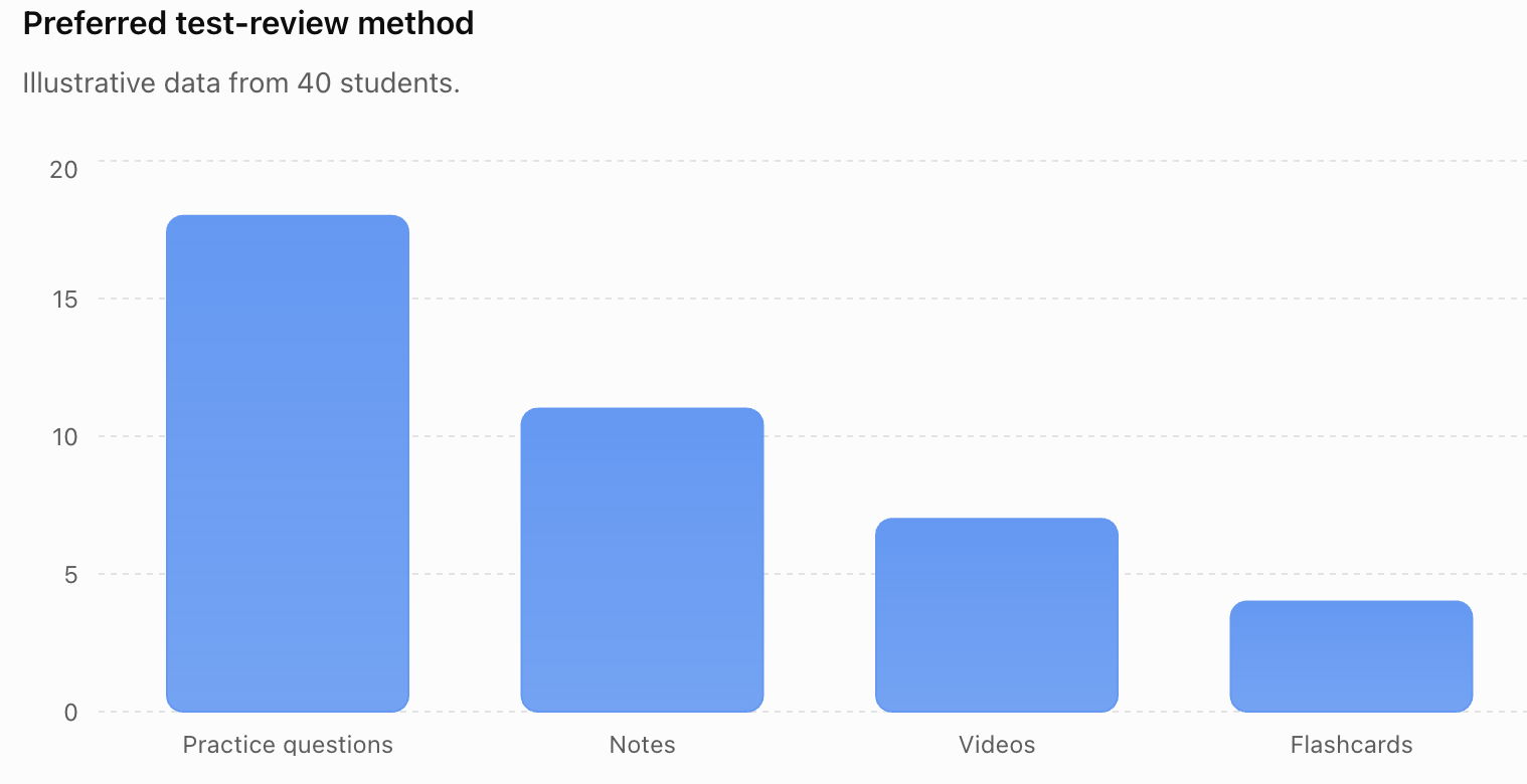
The graph should then be interpreted in words.

For example:

Practice questions were the most commonly selected review method, chosen by 18 of the 40 students.

Histograms

A histogram is useful for examining the distribution of numerical measurements.

For example, travel times could be grouped into intervals:

0–9 minutes
10–19 minutes
20–29 minutes
30–39 minutes
40–49 minutes
50–59 minutes

A histogram can reveal:

• typical values
• spread
• skewness
• clusters
• gaps
• possible outliers

 

 

 

5

Box Plots

Box plots are especially useful when comparing groups.

For example, you might compare:

sleep duration for Grade 9 students

with:

sleep duration for Grade 11 students

A box plot can show differences in:

• median
• IQR
• overall spread
• possible outliers

 

 

 

5

A strong analysis describes these differences numerically rather than simply saying that the graphs "look different."

Investigating Relationships with Scatter Plots

Suppose your project asks:

"Is there an association between study time and test score?"

Collect paired data:

Study Time	Test Score (%)
1.0	58
1.5	62
2.0	68
2.5	67
3.0	75
3.5	79
4.0	83
4.5	87

A scatter plot helps reveal the relationship.

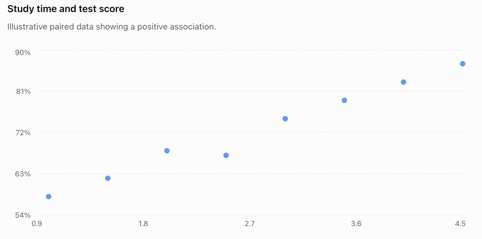
The data show a positive association:

students who studied longer tended to have higher scores in this illustrative data set.

But this does not automatically establish causation.

---

Correlation and Causation

Suppose your data show:

more sleep ↔ higher test scores

You should not automatically conclude:

more sleep caused higher test scores.

Other variables may include:

• study habits
• stress
• attendance
• health
• workload
• motivation

If your investigation is observational, a more appropriate conclusion is:

"Greater reported sleep duration was associated with higher test scores in the sample."

This describes what the evidence actually shows.

---

Using Probability in a Capstone Project

A capstone investigation can also focus on probability.

For example:

"Does this spinner behave according to its theoretical probabilities?"

Suppose a spinner has four equal sections.

The theoretical probability of each colour is:

1/4 = 25%

If it is spun 200 times, the expected frequency for each colour is:

200 × 1/4 = 50

Students can compare theoretical and experimental results.

 

 

 

7

---

Theoretical and Experimental Probability

Suppose 200 spins produce:

Colour	Theoretical	Observed
Red	50	54
Blue	50	46
Green	50	52
Yellow	50	48

The results are not exactly equal.

That is expected because of random variation.

Experimental probability for red:

54/200 = 0.27 = 27%

Theoretical probability:

25%

The difference alone does not prove that the spinner is biased.

---

Expected Value Investigations

Another possible project is to design or evaluate a game.

Suppose a game costs:

$2 to play

Possible outcomes are:

Outcome	Probability	Prize
A	1/10	$10
B	2/10	$3
C	7/10	$0

Expected winnings:

E(X) = 10(1/10) + 3(2/10) + 0(7/10)

= 1 + 0.60

= $1.60

Expected net gain:

1.60 − 2.00

= −$0.40

Therefore, the player expects to lose:

$0.40 per play in the long run.

This could form the basis of an investigation into whether a game is mathematically fair.

---

Comparing Theoretical Predictions with Data

Probability projects can combine theory and experimentation.

For example:

1. Calculate theoretical probabilities.
2. Predict expected frequencies.
3. Conduct the experiment.
4. Record observed frequencies.
5. Calculate experimental probabilities.
6. Compare theoretical and experimental results.
7. Explain differences using random variation.
8. Evaluate whether the number of trials was sufficient.

This connects probability directly with statistical investigation.

---

Looking for Outliers

An outlier should be investigated rather than automatically removed.

Suppose most travel times are:

15–50 minutes

but one student reports:

180 minutes

Possible explanations include:

• the student genuinely travels a very long distance
• the student misunderstood the question
• the value was entered incorrectly
• unusual circumstances affected the journey

The correct response is not simply:

"Delete the outlier."

Instead ask:

Why is it unusual, and how does it affect the analysis?

---

Comparing Results With and Without an Outlier

Consider:

10, 12, 13, 14, 15, 16, 18, 80

Mean:

178/8 = 22.25

Median:

(14 + 15)/2 = 14.5

The value 80 has strongly increased the mean.

If 80 is a genuine observation, this is important information about the distribution.

The median may provide a better measure of a typical value, but the unusual observation should still be discussed.

---

Drawing Evidence-Based Conclusions

A conclusion should answer the original research question using actual evidence.

Weak conclusion:

"Students don't sleep much."

Better conclusion:

"The median reported sleep duration among the 120 sampled students was 6.9 hours, while the mean was 6.8 hours."

Stronger:

"The median reported sleep duration among the 120 sampled students was 6.9 hours. About 68% reported fewer than eight hours, suggesting that sleep durations below eight hours were common in this sample."

The conclusion becomes stronger because it refers directly to evidence.

---

Separate Results from Interpretation

It is useful to distinguish between:

Result:
"The median travel time was 31 minutes."

and:

Interpretation:
"This suggests that a typical student in the sample spent about half an hour travelling to school."

and:

Conclusion:
"The sample therefore provides evidence that travel times of approximately 30 minutes are typical among the students represented by the investigation."

These statements are related, but they perform different roles.

---

Avoid Overgeneralization

Suppose you survey 30 students from one Grade 10 class.

Your evidence applies directly to:

those 30 students.

It may provide some information about other Grade 10 students, but the ability to generalize depends on how representative the sample is.

It would be inappropriate to claim:

"Teenagers everywhere sleep 6.8 hours."

The conclusion must remain within the limits of the evidence.

---

Communicating Findings with Tables

Tables are useful when readers need exact values.

For example:

Statistic	Sleep Duration
Sample size	120
Mean	6.8 h
Median	6.9 h
Q₁	6.2 h
Q₃	7.5 h
IQR	1.3 h
Minimum	4.5 h
Maximum	9.5 h

A table gives precise numerical information.

A graph can then help readers see the overall pattern.

---

Communicating Findings with Graphs

A good graph should be:

accurate

clearly labelled

easy to interpret

appropriate for the data

directly relevant to the research question

Avoid:

• unnecessary 3-D effects
• misleading scales
• missing units
• excessive decoration
• too many unrelated graphs

The goal is communication, not decoration.

---

Combining Graphs and Statistical Summaries

Strong statistical communication often combines several forms of evidence.

For example:

Histogram

Shows the shape of the distribution.

Median

Describes a typical value.

IQR

Describes the spread of the middle half.

Sample size

Shows how much data were collected.

Written interpretation

Explains what these results mean.

No single graph or statistic usually tells the complete story.

---

Writing the Final Report

A complete capstone report can be organized into the following sections.

Research Question

Clearly state what you investigated.

Background and Purpose

Explain why the question is interesting or useful.

Method

Explain:

• population
• sample
• sampling method
• variables
• collection procedure

Data

Present organized data or an appropriate summary.

Analysis

Include appropriate:

• graphs
• tables
• measures of centre
• measures of spread
• percentages
• probability calculations
• comparisons
• relationships

Findings

Describe the important patterns.

Conclusion

Answer the research question using evidence.

Evaluation

Discuss strengths, weaknesses, uncertainty, and improvements.

---

Evaluating Strengths

A strong investigation might have:

• a clearly defined research question
• an appropriate sample
• sufficient data
• consistent measurements
• neutral survey questions
• appropriate statistical calculations
• suitable graphs
• conclusions supported by evidence
• transparent reporting

Do not simply write:

"My project was good."

Identify specific strengths.

For example:

"A strength of the investigation was the use of stratified sampling across six grade levels, which reduced the risk that one grade would dominate the sample."

---

Evaluating Limitations

Every real investigation has limitations.

Possible limitations include:

• small sample size
• convenience sampling
• voluntary response
• non-response
• inaccurate measurements
• self-reported data
• unclear survey questions
• limited time
• missing data
• uncontrolled variables
• measurement precision
• unusual observations
• restricted population

A limitation should explain how it could affect the conclusion.

Weak:

"The sample was small."

Better:

"Only 25 students participated, so random differences between individuals may have had a relatively large effect on the sample statistics."

---

Self-Reported Data

Many student investigations use self-reported information.

For example:

"How many hours did you sleep last night?"

A participant may:

• forget
• estimate incorrectly
• round the answer
• misunderstand the question
• report what seems socially acceptable

Therefore, self-reported data should often be identified as a limitation.

---

Bias

Bias is a systematic influence that can move results away from an accurate representation of the population.

Possible forms include:

• selection bias
• voluntary response bias
• non-response bias
• wording bias
• measurement bias

 

 

 

6

Identifying bias is not simply a criticism of the project.

It demonstrates understanding of the quality of the evidence.

---

Random Variation Versus Bias

These ideas should not be confused.

Random variation causes unpredictable differences from sample to sample.

Bias systematically pushes results in a particular direction.

Increasing sample size generally helps reduce sampling variability.

However, simply collecting more observations does not necessarily remove bias.

A sample of 10,000 badly selected people can still be biased.

---

Reliability and Validity

Reliability asks:

Would the method give reasonably consistent results if repeated?

Validity asks:

Does the method actually measure what we intended to investigate?

For example, suppose we want to measure physical fitness using only student height.

Height can be measured very reliably.

But height is not a valid measure of overall fitness.

A strong project considers both reliability and validity.

---

Uncertainty

Statistical conclusions are rarely perfectly certain.

Sources of uncertainty include:

• sampling variation
• measurement error
• random processes
• missing data
• model assumptions

Appropriate statistical language includes:

"The data suggest..."

"The sample provides evidence that..."

"There appears to be an association..."

"Within this sample..."

This is not weak writing. It accurately represents what statistical evidence can establish.

---

Improving the Investigation

After identifying a limitation, propose a realistic improvement.

Limitation	Possible Improvement
Sample too small	Collect data from more participants
Convenience sample	Use random or stratified sampling
Leading question	Rewrite using neutral language
Measurement inconsistency	Standardize the procedure
One measurement per person	Use repeated measurements
Missing groups	Include participants from those groups
Self-reported measurements	Use direct measurement where practical
Short investigation period	Collect data over a longer period

Good evaluation connects each weakness to a practical improvement.

---

A Complete Example

Question

Is there an association between sleep duration and recreational screen time among Grade 10 students?

Plan

Population:

Grade 10 students at the school.

Sample:

80 students selected from several Grade 10 classes.

Variables:

• reported sleep duration in hours
• reported recreational screen time in hours

Collection

Students complete an anonymous questionnaire.

Organization

Responses are entered into a spreadsheet with one student per row.

Analysis

Calculate:

• mean and median sleep duration
• mean and median screen time
• range and IQR
• scatter plot
• possible correlation pattern

Possible Finding

Students reporting higher screen time tend to report somewhat lower sleep duration.

Appropriate Conclusion

"The sample showed a negative association between reported recreational screen time and reported sleep duration."

Inappropriate Conclusion

"Phones cause students to sleep less."

The investigation is observational and cannot establish that causal claim by itself.

Limitations

• self-reported data
• possible non-response
• other variables were not controlled
• data came from one school
• screen-time estimates may be inaccurate

Improvements

Future investigations could use:

• larger samples
• data from several schools
• device-recorded screen time
• sleep tracking
• additional variables such as workload or exercise

This turns a simple data collection exercise into a complete statistical investigation.

---

Capstone Project Workflow

A practical workflow is:

Choose a meaningful statistical question.

Plan the population, sample, variables, and method.

Predict what you think the data might show, if appropriate.

Collect the data carefully.

Check the data for errors and missing values.

Organize the data into useful tables.

Calculate appropriate statistical summaries.

Visualize the data using suitable graphs.

Analyze patterns, differences, distributions, or relationships.

Interpret what those patterns mean.

Conclude using evidence.

Evaluate strengths, limitations, uncertainty, and bias.

Improve the investigation by suggesting realistic changes.

Present the findings clearly.

 

 

 

4

---

Suggested Capstone Project Checklist

Before submitting a project, check that you can answer yes to most of these questions:

• Is my research question clearly stated?
• Is it genuinely statistical?
• Have I identified my population?
• Have I explained how my sample was selected?
• Have I identified my variables?
• Did I collect relevant data?
• Did I organize and check my data?
• Did I use appropriate statistical summaries?
• Did I choose appropriate graphs?
• Are my graphs correctly labelled?
• Did I interpret the graphs rather than simply include them?
• Did I answer the original research question?
• Did I support my conclusion with numerical evidence?
• Did I distinguish correlation from causation?
• Did I discuss possible bias?
• Did I identify limitations?
• Did I suggest realistic improvements?
• Are my conclusions no stronger than the evidence allows?

---

Common Mistakes

Starting without a clear research question

Collecting random data and deciding what to investigate afterward often produces a weak project.

Collecting data that do not answer the question

Every variable should have a purpose.

Using a biased sample

Convenient data are not necessarily representative data.

Using every possible statistical calculation

More calculations do not automatically create a better analysis. Choose statistics that help answer the question.

Choosing inappropriate graphs

Match the graph to the type of data and the purpose of the analysis.

Reporting graphs without interpreting them

Explain what the patterns actually mean.

Ignoring spread

Two groups can have similar averages but very different variability.

Deleting outliers automatically

Investigate unusual observations before deciding how to treat them.

Confusing association with causation

Observational data generally cannot establish causation by themselves.

Making claims beyond the population studied

A small sample from one school does not necessarily represent all teenagers.

Hiding inconvenient results

A statistical investigation should report the evidence honestly, even when the results do not support the original prediction.

Ignoring limitations

Recognizing limitations strengthens the investigation because it demonstrates critical statistical reasoning.

---

Key Terms

Capstone project — a culminating investigation that combines multiple skills and concepts into a complete study.

Statistical investigation — a systematic process of answering a question using data.

Research question — the specific question an investigation attempts to answer.

Population — the complete group about which conclusions are intended.

Sample — the subset of the population from which data are collected.

Representative sample — a sample that reasonably reflects important characteristics of the population.

Variable — a characteristic that can take different values.

Categorical data — observations classified into groups or categories.

Numerical data — observations represented by numerical measurements or counts.

Frequency — the number of times an outcome or category occurs.

Relative frequency — the proportion of observations belonging to an outcome or category.

Mean — the sum of numerical observations divided by their number.

Median — the middle observation in ordered data.

Mode — the most frequently occurring value or category.

Range — the difference between the maximum and minimum.

Interquartile range (IQR) — Q₃ − Q₁, describing the spread of the middle 50% of observations.

Distribution — the overall pattern of values in a data set.

Outlier — an observation unusually distant from the rest of the data.

Correlation — a statistical association between variables.

Expected frequency — the number of occurrences predicted from a probability model over a specified number of trials.

Expected value — the probability-weighted average numerical outcome of a random process.

Bias — a systematic influence that can distort results.

Random variation — natural unpredictable differences produced by sampling or random processes.

Reliability — the consistency of measurements or procedures.

Validity — the extent to which an investigation measures what it intends to measure.

Limitation — a feature of an investigation that restricts the strength or generalizability of its conclusions.

---

Key Takeaways

• A capstone data project combines the complete statistical investigation process in one independent study.
• Strong investigations begin with specific, measurable statistical questions.
• Planning should occur before data collection.
• The population, sample, sampling method, and variables should be clearly identified.
• Representative sampling is important when making conclusions about a population.
• Data should be collected consistently and checked before analysis.
• Statistical tools should be selected according to the question and type of data.
• Measures of centre describe typical values, while measures of spread describe variability.
• Graphs and tables should clarify the evidence rather than simply decorate the presentation.
• Scatter plots can reveal associations, but association alone does not establish causation.
• Probability investigations can compare theoretical probabilities, expected outcomes, and experimental results.
• Conclusions should answer the original question and refer directly to numerical or graphical evidence.
• Strong conclusions acknowledge uncertainty.
• Limitations should explain how weaknesses could affect the results.
• Improvements should directly address identified limitations.
• A successful capstone project demonstrates not only the ability to calculate statistics but the ability to use data to reason, evaluate evidence, and communicate a justified conclusion.

---

Check Your Understanding

1. Explain why a capstone data project should begin with a research question rather than simply collecting interesting data.
2. Rewrite "Are teenagers unhealthy?" as a specific statistical question that could realistically be investigated.
3. A student wants to investigate travel time among all students at a school but surveys only 20 students from their homeroom. Identify a limitation and suggest an improvement.
4. Explain why increasing the size of a strongly biased sample does not necessarily solve the problem.
5. For each variable, classify it as categorical, discrete numerical, or continuous numerical: transportation method, number of siblings, height, favourite subject, daily screen time.
6. A data set contains 12, 14, 15, 16, 16, 17, 18, 82. Explain why the mean and median may give very different impressions of a typical value.
7. Explain when you would choose a bar graph, histogram, box plot, and scatter plot.
8. Two groups have the same median but very different IQRs. What does this tell you about the groups?
9. A scatter plot shows that students who report more exercise also report higher happiness scores. Write an appropriate statistical conclusion that does not incorrectly claim causation.
10. A spinner is designed so that P(red) = 0.40. Calculate the expected number of red results in 500 spins. Explain why the actual number does not have to equal this value exactly.
11. A student finds an unexpected outlier and immediately deletes it. Explain why this is poor statistical practice.
12. Explain the difference between random variation and bias. Which problem can usually be reduced by increasing the sample size?
13. Design a capstone investigation involving two numerical variables. State your research question, population, sample, variables, collection method, appropriate graph, and at least two statistical summaries you would use.
14. Suppose your results do not support your original prediction. Explain what you should do when writing the final report.
15. Imagine that you have completed your capstone project. Write an outline for the final presentation showing how you would communicate your question, method, data, graphs, statistical analysis, conclusion, strengths, limitations, and possible improvements.
16.