Two-Dimensional Motion
5. Kinematics in Sports and Engineering
Learning outcomes
- I can identify examples of projectile motion in sports.
- I can explain how engineers use kinematics to design systems and structures.
- I can analyze motion in real-world applications using physics principles.
- I can evaluate how launch angle and speed affect projectile performance.
- I can apply kinematic concepts to practical and technological situations.
Kinematics in Sports and Engineering
Learning targets
- I can identify examples of projectile motion in sports.
- I can explain how engineers use kinematics to design systems and structures.
- I can analyze motion in real-world applications using physics principles.
- I can evaluate how launch angle and speed affect projectile performance.
- I can apply kinematic concepts to practical and technological situations.
Why is kinematics useful?
Kinematics describes motion using quantities such as:
- Position and displacement.
- Distance travelled.
- Speed and velocity.
- Acceleration.
- Time.
In sports, kinematics helps athletes and coaches analyze performance. In engineering, it helps designers predict how machines, vehicles and structures will behave.
Kinematic analysis can answer practical questions such as:
- How high will a ball travel?
- Will a projectile clear an obstacle?
- Where should a conveyor deposit its material?
- How much distance does a vehicle need to stop?
- How quickly should an elevator accelerate?
- When must a robotic arm begin slowing down?
- How far will an object travel after leaving a ramp?
Building a useful model
A real situation must be simplified before equations can be applied.
A kinematic model may assume:
- Motion occurs along a straight line.
- Acceleration remains constant.
- Air resistance is negligible.
- Gravitational acceleration is constant.
- An object can be represented as a single point.
- The surface is level.
- The launch and landing heights are known.
A model does not reproduce every detail of reality. It focuses on the factors needed to answer a particular question.
Projectile motion in sports
Many sports involve projectiles:
- A basketball travelling towards the hoop.
- A football kicked through the air.
- A javelin after release.
- A volleyball serve.
- A golf ball after impact.
- A baseball after being hit or thrown.
- An athlete’s centre of mass during a long jump.
After release, an ideal sports projectile has:
- Constant horizontal velocity.
- Constant downward acceleration.
- A curved parabolic trajectory.


Real sports projectiles are also affected by air resistance, spin, shape and wind. The ideal model provides a useful starting point.
Horizontal and vertical components
For a launch speed u at an angle θ above the horizontal:
uₓ = u cos θ
uᵧ = u sin θ
When air resistance is ignored:
aₓ = 0
aᵧ = −g
The horizontal motion is:
x = uₓt
The vertical motion is:
y = y₀ + uᵧt − ½gt²
Horizontal and vertical calculations share the same time.
How launch angle changes performance
Increasing the launch angle gives more of the initial velocity to the vertical component and less to the horizontal component.
Low launch angle
A low angle produces:
- A large horizontal component.
- A small vertical component.
- A low trajectory.
- A short flight time.
- Possible difficulty clearing obstacles.
High launch angle
A high angle produces:
- A smaller horizontal component.
- A larger vertical component.
- A higher trajectory.
- A longer flight time.
- Greater sensitivity to wind and drag.
Intermediate launch angle
An intermediate angle balances horizontal and vertical motion.
For an ideal projectile launched and landing at the same height:
R = u²sin(2θ)/g
The maximum theoretical range occurs at 45°.
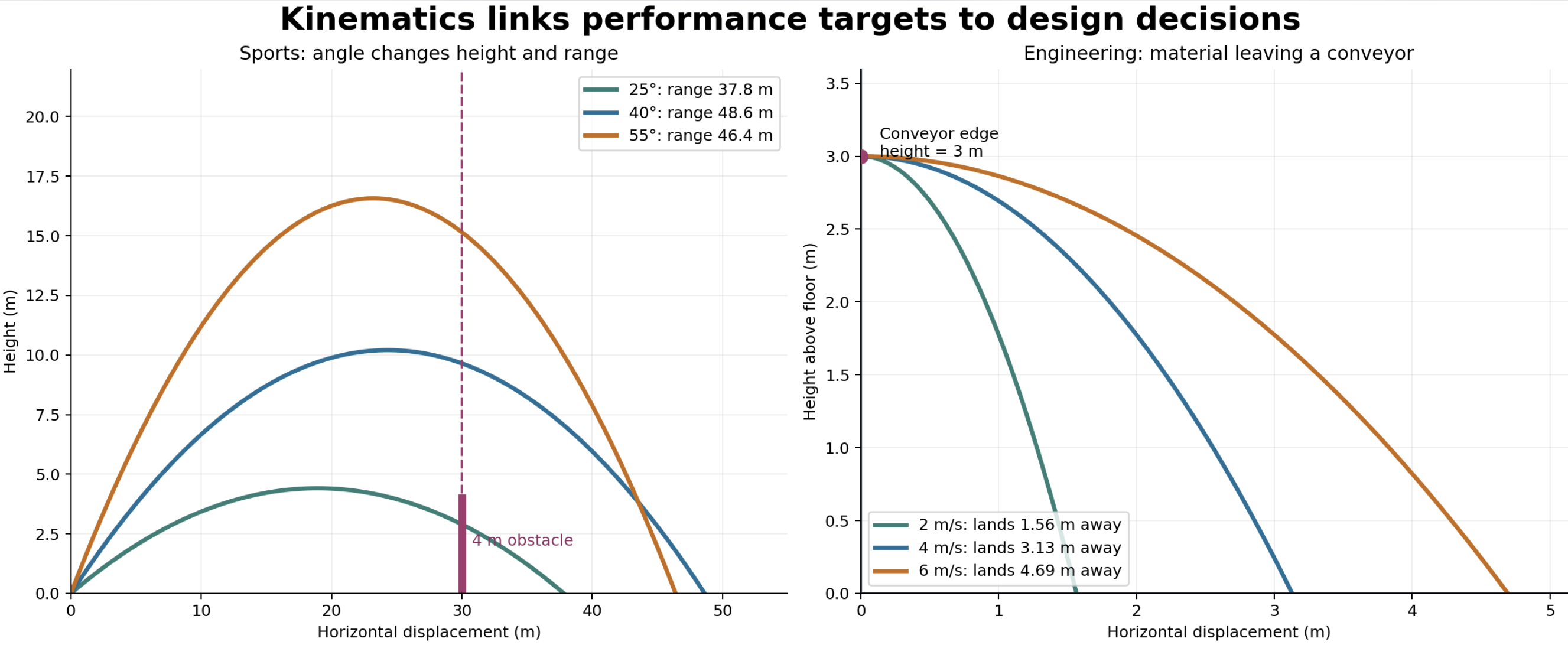
The sports graph compares projectiles launched at the same speed. The engineering graph shows that increasing conveyor speed increases the horizontal landing distance without changing the fall time.
Analyzing the sports graph
Each projectile is launched at 22 m/s from ground level.
| Launch angle | Approximate range | General trajectory |
|---|---|---|
| 25° | 37.8 m | Low and relatively short |
| 40° | 48.6 m | Moderate height and greatest of these ranges |
| 55° | 46.4 m | High with a long flight time |
A 4 m obstacle is positioned 30 m from the launch point.
- The 25° projectile is below the obstacle and does not clear it.
- The 40° projectile clears it.
- The 55° projectile clears it by a larger vertical distance.
- A higher path is not automatically the best path if range, travel time or accuracy also matters.
The most useful trajectory depends on the performance goal.
Worked example: clearing a defensive wall
A football is kicked at 22 m/s at 40° above the horizontal. A defensive wall 4.0 m high is located 30 m away. Determine whether the ball clears the wall. Ignore air resistance and use g = 9.8 m/s².
Resolve the launch velocity
uₓ = 22 cos 40°
uₓ ≈ 16.9 m/s
uᵧ = 22 sin 40°
uᵧ ≈ 14.1 m/s
Find the time to reach the wall
Horizontal motion has constant velocity:
x = uₓt
t = x/uₓ
t = 30/16.9
t ≈ 1.78 s
Find the ball’s height
y = uᵧt − ½gt²
y = 14.1(1.78) − 4.9(1.78²)
y ≈ 25.1 − 15.5
y ≈ 9.6 m
Find the clearance
Clearance = 9.6 − 4.0
Clearance = 5.6 m
The ideal model predicts that the ball clears the wall by approximately 5.6 m.
The calculation does not determine whether the shot enters the goal. That would require the goal’s position, the ball’s later trajectory and possibly the goalkeeper’s motion.
Launch speed and performance
Launch speed has a strong effect on projectile performance.
For equal launch and landing heights:
R = u²sin(2θ)/g
Therefore:
Range is proportional to the square of launch speed.
If launch speed doubles while the angle remains constant, the ideal range becomes four times as large.
Maximum height also depends on the square of the vertical launch speed:
H = uᵧ²/(2g)
A small increase in launch speed can therefore produce a substantial increase in height and range.
However, faster motion also makes air resistance more significant.
Worked example: effect of increasing launch speed
Two balls are launched at 45° from ground level.
- Ball A is launched at 15 m/s.
- Ball B is launched at 20 m/s.
Use g = 9.8 m/s².
At 45°, sin 90° = 1.
For Ball A:
R = 15²/9.8
R ≈ 23.0 m
For Ball B:
R = 20²/9.8
R ≈ 40.8 m
The speed increases by approximately 33%, but the ideal range increases by approximately 77%.
Basketball trajectory
A basketball shot must satisfy several conditions:
- Reach the horizontal position of the hoop.
- Be high enough to pass over the rim.
- Enter at a suitable downward angle.
- Avoid excessive speed that could cause it to rebound strongly.
- Clear defenders.


A higher release point reduces the required vertical rise. A steeper downward entry can increase the effective opening through the rim, although it may require a higher trajectory.
A real shot is also affected by backspin and air resistance.
Javelin and throwing events
A javelin is not a simple point projectile.
Its flight depends on:
- Release speed.
- Release angle.
- Release height.
- Aerodynamic lift and drag.
- Angle of attack.
- Wind.
- Orientation at landing.
A basic projectile model helps estimate the importance of speed, angle and height. More advanced analysis uses aerodynamic forces and computer simulation.
The ideal 45° maximum-range result does not give the best real javelin release angle because aerodynamic effects and release conditions change the motion.
Long jump and jumping sports
An athlete’s centre of mass behaves approximately like a projectile after take-off.
Coaches may measure:
- Take-off speed.
- Horizontal and vertical velocity components.
- Time in the air.
- Maximum height.
- Landing distance.
The athlete can move their arms and legs during flight, but these movements do not greatly change the projectile path of the whole body’s centre of mass once airborne.
They can, however, change body orientation and help position the feet for landing.
Engineering and projectile motion
Projectile calculations are used when an object leaves a moving system and travels through the air.
Examples include:
- Material leaving a conveyor belt.
- Water leaving a pipe or fountain.
- Packages released from moving equipment.
- Components moving between production stations.
- Emergency supply drops.
- Test objects launched during safety trials.


Engineers need to predict the landing position so that containers, barriers and other equipment can be placed safely.
Conveyor-release model
Suppose material leaves a horizontal conveyor 3.0 m above the floor.
The initial vertical velocity is zero:
uᵧ = 0
The vertical fall time is:
y = ½gt²
t = √(2y/g)
t = √[2(3.0)/9.8]
t ≈ 0.782 s
The fall time is determined by the height and gravity. It does not depend on the horizontal conveyor speed in the ideal model.
Horizontal landing distance is:
x = uₓt
| Conveyor speed | Fall time | Landing distance |
|---|---|---|
| 2 m/s | 0.782 s | 1.56 m |
| 4 m/s | 0.782 s | 3.13 m |
| 6 m/s | 0.782 s | 4.69 m |
Increasing conveyor speed increases the horizontal distance but does not change the fall time.
Worked engineering problem
A conveyor moves packages horizontally at 3.5 m/s. The packages leave the belt 1.8 m above the centre of a collection bin. Where should the bin be positioned? Ignore air resistance.
Find the fall time
Choose downward as positive.
uᵧ = 0 m/s
y = 1.8 m
aᵧ = 9.8 m/s²
Use:
y = ½aᵧt²
1.8 = 4.9t²
t² = 1.8/4.9
t ≈ 0.606 s
Find the horizontal distance
x = uₓt
x = 3.5(0.606)
x ≈ 2.12 m
The centre of the bin should be approximately 2.12 m horizontally from the conveyor edge under the ideal model.
In practice, engineers would allow for package size, rotation, air resistance and variation in conveyor speed.
Water fountains and fluid streams
A stream of water leaving a nozzle can follow an approximately projectile-shaped path.
Engineers can adjust:
- Nozzle speed.
- Nozzle angle.
- Nozzle height.
- Target landing position.
- Pump pressure.


Individual water droplets follow projectile paths after leaving the nozzle, although drag and interaction between droplets make a real stream more complex.
Transportation engineering
Kinematics is essential in vehicle and road-system design.
Engineers analyze:
- Acceleration lanes.
- Braking distances.
- Railway stopping zones.
- Elevator motion.
- Roller-coaster speeds.
- Vehicle collision tests.
- Runway lengths.
- Traffic-signal timing.
Stopping distance
Total stopping distance consists of:
Thinking distance + braking distance
Thinking distance is:
dₜ = utᵣ
For uniform braking:
v² = u² + 2as
When the vehicle stops, v = 0.
A greater initial speed increases both thinking and braking distances.
Worked example: runway stopping distance
An aircraft touches down at 70 m/s and decelerates uniformly at 3.5 m/s². Estimate the runway distance required to stop.
Choose the direction of motion as positive:
u = 70 m/s
v = 0 m/s
a = −3.5 m/s²
Use:
v² = u² + 2as
0 = 70² + 2(−3.5)s
0 = 4900 − 7s
s = 700 m
The ideal model predicts a braking distance of 700 m.
A real runway must provide additional distance for:
- Pilot response.
- Weather conditions.
- Variable braking.
- Safety margins.
- Aircraft mass and configuration.
- Possible rejected landings or emergencies.


Engineering design uses conservative safety margins rather than treating the ideal calculation as the exact required runway length.
Elevator and ride design
Elevators and amusement rides involve several motion stages:
- Acceleration.
- Constant velocity.
- Deceleration.
- Rest.
Engineers must consider both travel time and passenger comfort.
A very large acceleration can produce uncomfortable forces. A sudden change in acceleration, called jerk, can also be uncomfortable even if the acceleration itself remains within acceptable limits.
Motion controllers vary motor output to create a smooth velocity profile.
Robotics and automated systems
Robotic systems use kinematics to control:
- Position.
- Velocity.
- Acceleration.
- Timing.
- Collision avoidance.
- Tool paths.


A robotic arm must arrive at the correct position with an appropriate velocity. If it moves too quickly, it may overshoot, damage a component or create a safety hazard.
Sensors measure actual motion, and a controller compares the measurements with the planned motion.
Interpreting motion graphs in engineering
Position–time graphs
The gradient gives velocity.
Engineers can use the graph to determine:
- When a system reaches a particular position.
- Whether motion is smooth.
- Whether an object stops or reverses.
- Whether two components may collide.
Velocity–time graphs
The gradient gives acceleration, while area gives displacement.
The graph can show:
- Acceleration and braking stages.
- Maximum operating speed.
- Total travel distance.
- Reversal of direction.
Acceleration–time graphs
Area gives change in velocity.
The graph can reveal:
- Sudden impacts.
- Vibrations.
- Changes in machine operation.
- Passenger or product loads.
Using experimental data
Motion data can be collected using:
- High-speed video.
- Radar.
- GPS.
- Accelerometers.
- Light gates.
- Motion sensors.
- Timing gates.
- Computer vision.
Sports analysts may track a ball frame by frame. Engineers may place sensors on a vehicle, machine or structure.
Measured data can be compared with a mathematical model. Differences may reveal:
- Air resistance.
- Friction.
- Changing acceleration.
- Sensor uncertainty.
- Incorrect assumptions.
- Variation in human performance.
Evaluating a kinematic model
A good analysis does more than produce a numerical answer. It evaluates the model.
Ask:
- Is acceleration reasonably constant?
- Is air resistance significant?
- Are launch and landing heights equal?
- Is the object spinning?
- Are measurements sufficiently precise?
- Does the object have a complex shape?
- Is there wind?
- Does the model need a safety margin?
- Does the calculated result agree with observed motion?
A simple model may still be useful if its assumptions and limitations are stated clearly.
Ideal and real projectile paths
| Ideal model | Real motion |
|---|---|
| No air resistance | Drag reduces velocity |
| Perfect parabola | Path may be asymmetrical |
| Constant horizontal velocity | Horizontal velocity may decrease |
| Point-like object | Size, shape and orientation matter |
| No spin | Spin may create lift or sideways force |
| Still air | Wind may change the path |
The ideal model is valuable because it isolates the main relationships. More complex models build on it.
Safety factors in engineering
Engineering systems are rarely designed exactly to a theoretical minimum.
A calculated stopping distance of 700 m does not mean that a 700 m runway section is automatically sufficient. Engineers include safety factors to account for variation and uncertainty.
Safety margins may account for:
- Measurement uncertainty.
- Wear and maintenance.
- Weather.
- Material variation.
- Human response.
- Unexpected operating conditions.
- Model limitations.
A practical analysis method
- Identify the performance or design question.
- Draw and label the physical situation.
- Choose coordinate directions.
- State the assumptions.
- Identify known and unknown variables.
- Resolve vectors where necessary.
- Select suitable equations or graph methods.
- Calculate the required values.
- Compare the prediction with the performance target.
- Evaluate limitations and safety margins.
Common misconceptions
- “The greatest launch angle gives the greatest range.” Very high angles produce long flight times but small horizontal velocities.
- “A 45° angle is always best.” It gives maximum ideal range only for equal launch and landing heights without drag.
- “Increasing launch speed increases range by the same percentage.” Ideal range depends on speed squared.
- “A higher trajectory is always better.” The best path depends on the task.
- “The conveyor speed changes the fall time.” In the ideal model, fall time depends on vertical motion.
- “A calculated engineering value can be used without a safety margin.” Real conditions and uncertainty must be considered.
- “Sports projectiles follow perfect parabolas.” Air resistance and spin alter their paths.
- “Kinematics is used only for projectiles.” It applies to vehicles, elevators, robots and many other moving systems.
Did you know?
A golf ball’s dimples deliberately change the airflow around the ball. They reduce some forms of drag and help spin generate lift, allowing the ball to remain airborne longer than a smooth ball launched under similar conditions.
Its real flight therefore differs substantially from the simplest projectile model.
Key terms
- Sports biomechanics: The application of mechanical principles to human movement and sports.
- Projectile motion: Two-dimensional motion under gravity after launch.
- Launch angle: Direction of initial velocity relative to the horizontal.
- Launch speed: Magnitude of the initial velocity.
- Range: Horizontal displacement from launch to landing.
- Release height: Height of a projectile at launch.
- Trajectory: Path followed by a moving object.
- Kinematic model: A mathematical representation of motion.
- Motion sensor: A device used to measure position or motion.
- Safety factor: Extra design capacity added to account for uncertainty.
- Jerk: Rate of change of acceleration.
- Drag: A resistive force opposing motion through a fluid.
- Magnus force: A force caused by the motion and spin of an object through a fluid.
Key takeaways
- Many sports involve projectile motion after an object is released.
- Launch speed, angle and height affect maximum height, flight time and range.
- The best trajectory depends on the performance goal.
- Engineers use kinematics to predict landing positions, stopping distances and movement times.
- Conveyor-release problems combine horizontal constant velocity with vertical free fall.
- Sports and engineering data can be interpreted using motion graphs.
- Real motion may differ from ideal predictions because of drag, spin and changing acceleration.
- Engineering applications require assumptions, testing and safety margins.
- Kinematics connects mathematical models to practical decisions.