Applications and Connections
| Site: | Young Education |
| Cours: | Exponential and Logarithmic Functions |
| Livre: | Applications and Connections |
| Imprimé par: | Guest user |
| Date: | lundi, 9 novembre 2026, 16:38 |
1. Finance Applications
Learning outcomes
- I can solve compound interest problems.
- I can analyse investment growth.
- I can compare financial models.
- I can solve loan repayment problems.
- I can interpret financial data mathematically.
Introduction
Mathematics plays an essential role in financial decision-making. Whether we are saving money, investing for the future, borrowing to purchase a home, or comparing different loan offers, mathematical models help us understand how money changes over time.
Consider the following questions:
-
How much will $5,000 become after 10 years in a savings account?
-
Is an investment offering 6% annual interest necessarily better than one offering 5.9% interest compounded monthly?
-
How much should someone save each month to reach a financial goal?
-
Why can a long-term loan cost considerably more than the original amount borrowed?
-
How can we compare investments with different growth rates, fees, and risks?
These questions involve exponential functions, geometric sequences, logarithms, percentages, and mathematical modelling.
In this lesson, we will explore how mathematical models are used in personal finance, investment analysis, loan repayments, and the interpretation of financial data.
The goal is not simply to calculate financial values, but to understand what those calculations mean and how they can support informed decisions.
The Time Value of Money
One of the most important ideas in finance is the time value of money.
Money available today can be invested to earn a return, so it may be worth more than the same nominal amount received in the future.
For example, $1,000 invested at an annual return of 5% becomes:
After one year:
1,000 × 1.05 = $1,050
After two years:
1,050 × 1.05 = $1,102.50
After three years:
1,102.50 × 1.05 = $1,157.63
The amount increases because each year's growth is calculated using the previous year's balance.
This is the principle of compound interest.
The time value of money also depends on inflation, risk, and the opportunity cost of using money for one purpose rather than another.
Simple Interest
Simple interest is calculated only on the original principal.
The formula is:
I = Prt
Where:
-
I = interest earned.
-
P = principal or original amount.
-
r = annual interest rate as a decimal.
-
t = time in years.
The final amount is:
A = P(1 + rt)
Worked Example 1: Simple Interest
An investor deposits $4,000 at 5% simple annual interest for six years.
Calculate the interest and final amount.
Step 1: Identify the values.
P = 4000
r = 0.05
t = 6
Step 2: Calculate interest.
I = 4000 × 0.05 × 6
I = 1200
Step 3: Calculate the final amount.
A = 4000 + 1200
Final amount = $5,200
Simple interest produces linear growth because the same amount of interest is earned each year.
Compound Interest
Compound interest is calculated on the principal and previously accumulated interest.
With annual compounding:
A = P(1 + r)ⁿ
Where:
-
A = final amount.
-
P = initial principal.
-
r = annual interest rate as a decimal.
-
n = number of years.
Unlike simple interest, compound interest produces exponential growth.
Visualising compound interest
Explore compound investment growth
Explore how changing the principal, interest rate, and investment period affects compound growth. The model assumes a fixed rate and no additional contributions.Worked Example 2: Annual Compound Interest
An investor deposits $5,000 into an account paying 6% interest compounded annually.
Calculate the balance after 10 years.
Step 1: Identify the values.
P = 5000
r = 0.06
n = 10
Step 2: Substitute.
A = 5000(1.06)¹⁰
Step 3: Evaluate.
(1.06)¹⁰ ≈ 1.790848
A ≈ 5000 × 1.790848
A ≈ $8,954.24
Step 4: Calculate the interest earned.
Interest = 8954.24 − 5000
Interest ≈ $3,954.24
The investment earns approximately $3,954.24 over 10 years.
Simple Interest Versus Compound Interest
Consider $5,000 invested at 6% annually.
Simple interest increases by a constant amount each year.
Compound interest increases by a constant percentage each year.
Over longer periods, the difference becomes increasingly significant.
Compounding More Than Once Per Year
Interest may be compounded annually, semiannually, quarterly, monthly, or daily.
The general compound interest formula is:
A = P(1 + r/m)^(mt)
Where:
-
P = principal.
-
r = nominal annual interest rate.
-
m = number of compounding periods per year.
-
t = time in years.
The interest rate per compounding period is r/m.
The total number of compounding periods is mt.
Worked Example 3: Monthly Compounding
An investment of $8,000 earns 4.8% annual interest compounded monthly for five years.
Calculate the final amount.
P = 8000
r = 0.048
m = 12
t = 5
Substitute:
A = 8000(1 + 0.048/12)^(12 × 5)
A = 8000(1.004)⁶⁰
A ≈ 8000(1.27064)
A ≈ $10,165.12
The final amount is approximately $10,165.12.
The interest earned is approximately $2,165.12.
Continuous Compounding
Continuous compounding represents the limiting case as interest is compounded increasingly frequently.
The formula is:
A = Peʳᵗ
Where e ≈ 2.71828.
Worked Example 4: Continuous Compounding
A deposit of $10,000 earns 5% annual interest compounded continuously for eight years.
A = 10000e^(0.05 × 8)
A = 10000e⁰·⁴
A ≈ 10000(1.491825)
A ≈ $14,918.25
The interest earned is approximately $4,918.25.
Comparing Compounding Frequencies
For a nominal annual interest rate of 6%, an investment of $10,000 produces different balances after one year.
|
Compounding frequency |
Final amount |
|---|---|
|
Annually |
$10,600.00 |
|
Semiannually |
$10,609.00 |
|
Quarterly |
$10,613.64 |
|
Monthly |
$10,616.78 |
|
Daily (365 times) |
$10,618.31 |
|
Continuously |
$10,618.37 |
More frequent compounding increases the final amount when the nominal rate is positive.
However, the additional benefit becomes smaller as the frequency increases.
Continuous compounding does not mean unlimited interest. It produces a finite limiting value for any fixed principal, interest rate, and time period.
Effective Annual Interest Rate
Two financial products may advertise the same nominal annual interest rate but use different compounding frequencies.
To compare them fairly, we calculate the effective annual rate (EAR).
The formula is:
EAR = (1 + r/m)ᵐ − 1
Where:
-
r = nominal annual interest rate.
-
m = number of compounding periods per year.
For continuous compounding:
EAR = eʳ − 1
Worked Example 5: Comparing Savings Accounts
Bank A offers 5% interest compounded annually.
Bank B offers 4.9% interest compounded monthly.
Which account provides the higher effective annual rate?
Bank A
EAR = 0.05
EAR = 5%
Bank B
EAR = (1 + 0.049/12)¹² − 1
EAR ≈ 0.050115
EAR ≈ 5.012%
Conclusion
Bank B offers a slightly higher effective annual rate.
Although Bank B advertises a lower nominal rate, monthly compounding produces a marginally higher annual return.
This comparison assumes the same conditions and excludes fees, taxes, withdrawal restrictions, and other differences.
Investment Growth Over Time
Investments may grow through interest, dividends, capital appreciation, or a combination of these.
For a constant effective annual return r:
V(t) = V₀(1 + r)ᵗ
Where:
-
V₀ = initial investment.
-
r = effective annual return.
-
t = number of years.
Worked Example 6: Comparing Investment Growth
Two investments begin with $10,000.
Investment A earns 4% annually.
Investment B earns 7% annually.
Compare their values after 20 years.
Investment A:
A = 10000(1.04)²⁰
A ≈ $21,911.23
Investment B:
B = 10000(1.07)²⁰
B ≈ $38,696.84
Difference:
38,696.84 − 21,911.23
Difference ≈ $16,785.61
A difference of three percentage points in annual growth produces a substantial difference over 20 years.
However, higher expected returns are often associated with greater uncertainty or risk. Real investment returns are not generally constant or guaranteed.
The Rule of 72
The Rule of 72 provides a quick estimate of the time required for an investment to double.
Doubling time ≈ 72 ÷ annual growth rate (%)
For example, at 6% annual growth:
Doubling time ≈ 72/6
Doubling time ≈ 12 years
The exact doubling time for annual compounding is:
t = ln(2)/ln(1 + r)
At 6%:
t = ln(2)/ln(1.06)
t ≈ 11.90 years
The Rule of 72 provides a convenient approximation, but logarithms give a more accurate result.
Solving for Time Using Logarithms
Compound interest problems sometimes ask how long an investment must grow to reach a target amount.
Start with:
A = P(1 + r)ᵗ
Divide by P:
A/P = (1 + r)ᵗ
Take natural logarithms:
ln(A/P) = t ln(1 + r)
Therefore:
t = ln(A/P)/ln(1 + r)
Worked Example 7: Reaching a Savings Goal
An investor deposits $6,000 at 5% annual compound interest.
How long will it take to reach $10,000?
10000 = 6000(1.05)ᵗ
Divide by 6000:
1.666667 = (1.05)ᵗ
Take natural logarithms:
ln(1.666667) = t ln(1.05)
t = ln(1.666667)/ln(1.05)
t ≈ 10.47 years
If interest is credited only at the end of each year, the balance first reaches or exceeds $10,000 after 11 complete years.
Regular Savings Contributions
Many people invest regularly rather than depositing a single amount.
For equal payments made at the end of each period, the future value of an ordinary annuity is:
FV = PMT[(1 + i)ⁿ − 1]/i
Where:
-
FV = future value.
-
PMT = payment each period.
-
i = interest rate per period.
-
n = number of payments.
The formula assumes that payments and compounding occur at the same regular intervals and that the interest rate remains constant.
Worked Example 8: Monthly Retirement Savings
A person invests $250 at the end of each month for 20 years.
The account earns a nominal annual interest rate of 6%, compounded monthly.
Calculate the future value.
Step 1: Identify the values.
PMT = 250
Monthly rate:
i = 0.06/12 = 0.005
Number of payments:
n = 20 × 12 = 240
Step 2: Substitute.
FV = 250[(1.005)²⁴⁰ − 1]/0.005
Step 3: Evaluate.
(1.005)²⁴⁰ ≈ 3.31020
FV ≈ 250(2.31020/0.005)
FV ≈ $115,510.22
Step 4: Calculate total contributions.
250 × 240 = $60,000
Step 5: Calculate investment growth.
115510.22 − 60000
Growth ≈ $55,510.22
The account grows to approximately $115,510, of which $60,000 comes from contributions and the remainder from compounded returns.
This example assumes fixed returns and ignores taxes, fees, and inflation.
Understanding Loans and Repayments
A loan allows someone to borrow money and repay it over time, usually with interest.
Common examples include:
-
Home mortgages.
-
Car loans.
-
Personal loans.
-
Student loans.
-
Business loans.
Important loan terms include:
Principal: The amount originally borrowed.
Interest rate: The cost of borrowing, expressed as a percentage.
Loan term: The period over which the loan is repaid.
Repayment: The amount paid at each scheduled interval.
Outstanding balance: The amount still owed at a particular time.
How amortising loans work
An amortising loan is repaid through regular payments that cover interest and reduce the principal.
In a standard fixed-rate, fully amortising loan, the payments remain equal, but the proportion allocated to interest and principal changes over time.
At the beginning, the outstanding balance is relatively large, so the interest component is large.
As the principal decreases, less interest is charged each period, and more of each payment reduces the remaining principal.
The Loan Repayment Formula
For a loan with equal payments at the end of each period:
PMT = PV × i/[1 − (1 + i)⁻ⁿ]
Where:
-
PMT = regular repayment.
-
PV = present value, or amount borrowed.
-
i = interest rate per repayment period.
-
n = total number of repayments.
The formula assumes a constant interest rate, regular payment intervals, and no additional fees.
For monthly repayments with a nominal annual rate r compounded monthly:
i = r/12
n = 12t
where t is the loan term in years.
Worked Example 9: Calculating a Monthly Loan Repayment
A person borrows $20,000 at a nominal annual interest rate of 6%, compounded monthly.
The loan is repaid through equal monthly payments over five years.
Calculate the monthly repayment.
Step 1: Identify the values.
PV = 20000
Annual rate = 0.06
Monthly rate:
i = 0.06/12 = 0.005
Number of payments:
n = 5 × 12 = 60
Step 2: Substitute into the repayment formula.
PMT = 20000 × 0.005/[1 − (1.005)⁻⁶⁰]
Step 3: Evaluate.
(1.005)⁻⁶⁰ ≈ 0.74137
PMT ≈ 100/(1 − 0.74137)
PMT ≈ $386.66 per month
The borrower pays approximately $386.66 each month. The lender may adjust the final payment slightly because of rounding.
Calculating total interest
Total payments, using the rounded monthly payment:
60 × 386.66 = $23,199.60
Total interest:
23,199.60 − 20,000
Total interest ≈ $3,199.60
The borrower repays approximately $3,200 more than the original loan amount.
Understanding Loan Amortisation
An amortisation schedule shows how each repayment is divided between interest and principal.
For each period:
Interest = Outstanding balance × Periodic interest rate
Principal repaid = Payment − Interest
New balance = Previous balance − Principal repaid
Equivalently:
New balance = Previous balance(1 + i) − Payment
Worked Example 10: First Three Loan Payments
Consider the $20,000 loan with monthly repayments of approximately $386.66 and monthly interest rate 0.005.
First payment
Interest:
20000 × 0.005 = $100.00
Principal repaid:
386.66 − 100.00 = $286.66
New balance:
20000 − 286.66 = $19,713.34
Second payment
Interest:
19713.34 × 0.005 ≈ $98.57
Principal repaid:
386.66 − 98.57 = $288.09
New balance:
19713.34 − 288.09 = $19,425.25
Third payment
Interest:
19425.25 × 0.005 ≈ $97.13
Principal repaid:
386.66 − 97.13 = $289.53
New balance:
19425.25 − 289.53 = $19,135.72
|
Payment |
Payment amount |
Interest |
Principal repaid |
Balance |
|---|---|---|---|---|
|
0 |
— |
— |
— |
$20,000.00 |
|
1 |
$386.66 |
$100.00 |
$286.66 |
$19,713.34 |
|
2 |
$386.66 |
$98.57 |
$288.09 |
$19,425.25 |
|
3 |
$386.66 |
$97.13 |
$289.53 |
$19,135.72 |
Values are rounded to the nearest cent. An actual lender's amortisation schedule may differ slightly because of its rounding conventions.
Notice that the interest component decreases while the principal component increases.
This is why the outstanding loan balance decreases slowly at first and more quickly later.
Visualising Loan Repayment
The following graph shows an illustrative $20,000 loan at 6% nominal annual interest, repaid monthly over five years.
The graph curves downward because the amount of principal repaid each month increases as the interest component decreases.
Comparing Loan Terms
A longer loan term usually reduces the required monthly payment, but increases the total interest paid when the interest rate is unchanged.
Consider a $30,000 loan at a nominal annual interest rate of 6%, compounded monthly.
|
Loan term |
Monthly payment (approx.) |
Total interest (approx.) |
|---|---|---|
|
3 years |
$912.66 |
$2,856 |
|
5 years |
$579.98 |
$4,799 |
|
7 years |
$438.26 |
$6,814 |
The seven-year loan has the lowest monthly repayment, but the highest total interest cost.
The three-year loan has a higher monthly repayment but a lower total borrowing cost.
Interpreting the trade-off
A borrower must consider both affordability and overall cost.
A smaller monthly payment may be easier to manage, but it does not necessarily mean the loan is cheaper.
The best loan is not simply the loan with the lowest monthly repayment.
Other important factors include fees, effective interest rates, early repayment conditions, and whether the rate is fixed or variable.
Calculating the Outstanding Loan Balance
After several repayments, the outstanding balance can be calculated using:
Bₖ = PV(1 + i)ᵏ − PMT[(1 + i)ᵏ − 1]/i
Where:
-
Bₖ = balance after k payments.
-
PV = original loan amount.
-
i = interest rate per period.
-
PMT = regular payment.
-
k = number of payments made.
The first term represents how much the original loan would have grown through interest.
The second term represents the accumulated effect of repayments.
Worked Example 11: Outstanding Balance
A borrower takes out a $10,000 loan at 1% interest per month and makes payments of $300 at the end of each month.
Find the outstanding balance immediately after 12 payments.
PV = 10000
i = 0.01
PMT = 300
k = 12
Substitute:
B₁₂ = 10000(1.01)¹² − 300[(1.01)¹² − 1]/0.01
Since:
(1.01)¹² ≈ 1.126825
B₁₂ ≈ 11268.25 − 300(12.6825)
B₁₂ ≈ 11268.25 − 3804.75
B₁₂ ≈ $7,463.50
The borrower still owes approximately $7,463.50 after 12 payments.
The exact balance depends on the lender's interest and rounding rules.
Present Value and Discounting
Compound interest calculates how money grows into the future.
Present value works in the opposite direction.
It calculates how much a future amount is worth today under an assumed discount rate.
For annual compounding:
PV = FV/(1 + r)ⁿ
Where:
-
PV = present value.
-
FV = future value.
-
r = discount rate per period.
-
n = number of periods.
Worked Example 12: Present Value
An investment is expected to pay $15,000 in five years.
If the appropriate annual discount rate is 6%, calculate its present value.
PV = 15000/(1.06)⁵
PV = 15000/1.338226
PV ≈ $11,208.87
This means that approximately $11,208.87 invested today at 6% annually would grow to $15,000 after five years.
The present value depends on the discount rate selected.
Comparing Financial Models
Financial situations may involve linear, exponential, and annuity-based models.
|
Financial situation |
Mathematical model |
Important feature |
|---|---|---|
|
Simple interest |
Linear |
Constant interest earned per year |
|
Compound interest |
Exponential |
Interest earns additional interest |
|
Continuous compounding |
Natural exponential |
Limiting form of increasingly frequent compounding |
|
Regular savings |
Geometric series / annuity |
Repeated contributions accumulate |
|
Fixed-rate amortising loan |
Annuity present value |
Equal repayments reduce debt |
|
Inflation |
Often exponential |
Prices increase by a proportional rate |
|
Investment valuation |
Discounted cash flow |
Future payments converted to present values |
Choosing the correct model
Before selecting a formula, ask:
-
Is the interest simple or compounded?
-
Are payments made once or repeatedly?
-
Are payments made at the beginning or end of each period?
-
What is the interest rate per period?
-
How many periods are involved?
-
Is the rate fixed or variable?
-
Are fees, taxes, inflation, or other factors relevant?
Using the wrong model can produce a significantly incorrect financial result.
Inflation and Purchasing Power
Inflation refers to an increase in the general price level over time.
When prices rise, the purchasing power of a fixed amount of money decreases.
If inflation remains constant at rate f per year:
Future price = Current price × (1 + f)ᵗ
The purchasing power of a future nominal amount, expressed in today's money, is:
Real value = Future nominal value/(1 + f)ᵗ
Worked Example 13: Inflation
An item costs $1,000 today.
Assume prices increase by 3% annually for 10 years.
Calculate its expected price after 10 years.
Future price = 1000(1.03)¹⁰
Future price ≈ 1000(1.343916)
Future price ≈ $1,343.92
An item costing $1,000 today would cost approximately $1,343.92 after 10 years under this assumption.
Real Investment Returns
Suppose an investment earns an effective nominal annual return of 7%, while inflation is 3%.
The exact real annual return is:
Real return = (1 + nominal return)/(1 + inflation) − 1
Real return = 1.07/1.03 − 1
Real return ≈ 0.038835
Real return ≈ 3.88%
Although the investment grows by 7% in nominal terms, its purchasing power increases by approximately 3.88% per year.
This assumes the stated rates remain constant and ignores taxes and fees.
Interpreting Financial Data
Financial data should be interpreted mathematically rather than simply accepted at face value.
Important measures include:
-
Absolute change.
-
Percentage change.
-
Compound annual growth rate.
-
Effective interest rate.
-
Total interest paid.
-
Real return after inflation.
-
Volatility and uncertainty.
Percentage Change
Percentage change = [(New value − Old value)/Old value] × 100%
Suppose an investment increases from $8,000 to $9,200.
Percentage change:
(9200 − 8000)/8000 × 100%
= 1200/8000 × 100%
Percentage increase = 15%
Compound Annual Growth Rate (CAGR)
CAGR measures the constant annual growth rate that would produce the same beginning and ending values over a specified period.
CAGR = (Final value/Initial value)^(1/n) − 1
Worked Example 14: Calculating CAGR
An investment grows from $12,000 to $18,000 over six years.
Calculate its compound annual growth rate.
CAGR = (18000/12000)^(1/6) − 1
CAGR = 1.5^(1/6) − 1
CAGR ≈ 0.069913
CAGR ≈ 6.99% per year
This means the investment experienced the same overall growth as an investment increasing at approximately 6.99% every year.
It does not mean the actual return was 6.99% in each individual year.
Interpreting Investment Performance Graphs
Consider an investment with the following year-end values.
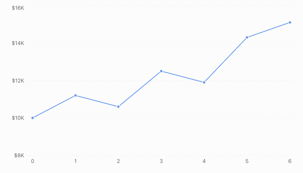
The investment increases overall from $10,000 to $15,100.
Total return:
(15100 − 10000)/10000 × 100%
Total return = 51%
However, the graph shows that growth was not constant.
The investment experienced declines in some years.
This illustrates an important limitation of using a single constant-rate exponential model for investment performance.
Mathematical questions to ask
When interpreting a financial graph, consider:
-
Is the vertical axis scaled appropriately?
-
Are values nominal or inflation-adjusted?
-
Does the graph include fees and dividends?
-
Are the time intervals consistent?
-
Does the graph show a long enough period?
-
Is the reported return an average, a compound annual rate, or a single-period return?
-
Does the model account for uncertainty and risk?
A graph showing strong historical growth does not guarantee similar future performance.
Financial Risk and Mathematical Modelling
Financial models often assume that interest rates and investment returns remain constant. Real financial markets are more complicated.
Investment values can fluctuate, interest rates can change, and unexpected events can affect financial outcomes.
Expected Return
Suppose an investment has three possible annual outcomes.
|
Outcome |
Probability |
Return |
|---|---|---|
|
Strong performance |
0.25 |
15% |
|
Moderate performance |
0.50 |
6% |
|
Poor performance |
0.25 |
−8% |
The expected return is calculated using a weighted average:
E(R) = Σ[pᵢ × Rᵢ]
Substitute:
E(R) = 0.25(15%) + 0.50(6%) + 0.25(−8%)
E(R) = 3.75% + 3% − 2%
Expected return = 4.75%
This does not mean the investment will earn exactly 4.75%.
It represents the probability-weighted average return under the assumed outcomes.
Risk and Return
Two investments may have the same expected return but different levels of risk.
For example, one investment might consistently earn returns close to 5%, while another experiences large gains and losses.
Measures such as standard deviation can help describe the variability of returns.
Financial decisions should therefore consider both expected return and uncertainty.
Authentic Application: Comparing Two Savings Plans
A student wants to save money for university expenses over the next 10 years.
Two savings plans are available.
Plan A
-
Initial deposit: $5,000
-
Nominal annual interest rate: 4.5%
-
Compounded annually
-
No additional contributions
Plan B
-
Initial deposit: $5,000
-
Nominal annual interest rate: 4.2%
-
Compounded monthly
-
No additional contributions
Which plan produces the larger balance after 10 years?
Step 1: Calculate Plan A
A = 5000(1.045)¹⁰
A ≈ 5000(1.55297)
Plan A ≈ $7,764.85
Step 2: Calculate Plan B
A = 5000(1 + 0.042/12)¹²⁰
A = 5000(1.0035)¹²⁰
A ≈ 5000(1.52089)
Plan B ≈ $7,604.45
Step 3: Compare the results
Difference:
7764.85 − 7604.45
Difference ≈ $160.40
Plan A produces approximately $160 more over 10 years under the stated assumptions.
Step 4: Interpret the result
Although Plan B compounds more frequently, Plan A offers a sufficiently higher nominal interest rate to produce a larger final balance.
This demonstrates why comparing compounding frequency alone is not enough.
A complete comparison should consider effective annual rates, fees, account conditions, and whether the advertised rates are guaranteed.
Authentic Application: Comparing Two Loan Offers
A borrower needs $25,000 to purchase a vehicle.
Two lenders offer fixed-rate loans with monthly compounding and payments.
|
Feature |
Loan A |
Loan B |
|---|---|---|
|
Principal |
$25,000 |
$25,000 |
|
Nominal annual rate |
5.5% |
6.2% |
|
Loan term |
5 years |
4 years |
|
Repayment frequency |
Monthly |
Monthly |
Loan A
Monthly rate:
i = 0.055/12
Number of payments:
n = 60
Monthly repayment:
PMT = 25000(0.055/12)/[1 − (1 + 0.055/12)⁻⁶⁰]
PMT ≈ $477.53
Total repayment:
Approximately $28,651.80
Total interest:
Approximately $3,651.80
Loan B
Monthly rate:
i = 0.062/12
Number of payments:
n = 48
Monthly repayment:
PMT = 25000(0.062/12)/[1 − (1 + 0.062/12)⁻⁴⁸]
PMT ≈ $589.46
Total repayment:
Approximately $28,294.08
Total interest:
Approximately $3,294.08
Comparing the loans
Loan A has a lower monthly repayment.
Loan B has a higher monthly repayment but a lower total interest cost because it is repaid more quickly.
The choice depends on the borrower's budget, financial priorities, and the full loan conditions.
The comparison excludes fees, insurance, and other possible charges.
Common Mistakes
Mistake 1: Confusing simple and compound interest
Simple interest is calculated only on the original principal.
Compound interest includes interest earned on previous interest.
Correction: Identify the interest calculation method before choosing a formula.
Mistake 2: Using a percentage instead of a decimal
Substituting 5 instead of 0.05 produces an incorrect result.
Correction: Divide percentage rates by 100.
Mistake 3: Mixing time units
Using an annual interest rate with monthly periods without conversion gives incorrect results.
Correction: Ensure the interest rate and number of periods use consistent units.
Mistake 4: Assuming more frequent compounding always means a better investment
A higher nominal rate with less frequent compounding may outperform a lower rate with more frequent compounding.
Correction: Compare effective annual rates.
Mistake 5: Confusing loan repayment with interest expense
Each loan repayment generally includes principal and interest.
Correction: Use an amortisation schedule to distinguish the components.
Mistake 6: Comparing loans only by monthly repayment
A longer loan may have smaller monthly payments but greater total interest.
Correction: Compare the full repayment cost and loan conditions.
Mistake 7: Ignoring inflation
An investment may increase in nominal value while gaining little purchasing power.
Correction: Calculate real returns where appropriate.
Mistake 8: Assuming investment returns are guaranteed
Constant-rate models are mathematical simplifications.
Correction: Consider variability, uncertainty, fees, and risk.
Mistake 9: Treating CAGR as the actual return every year
CAGR represents an equivalent constant annual rate.
Correction: Examine individual annual returns as well as overall growth.
Mistake 10: Assuming a lower advertised loan rate always means a cheaper loan
Fees, compounding conventions, and repayment terms can affect the total cost.
Correction: Compare effective rates and total borrowing costs on a consistent basis.
Key Terms
-
Principal: The original amount invested or borrowed.
-
Simple Interest: Interest calculated only on the original principal.
-
Compound Interest: Interest calculated on the principal and accumulated interest.
-
Compounding Period: The interval at which interest is added.
-
Nominal Interest Rate: The stated annual interest rate before adjusting for compounding frequency.
-
Effective Annual Rate (EAR): The actual annual rate after accounting for compounding.
-
Continuous Compounding: The limiting form of compounding as the frequency increases without bound.
-
Future Value: The value of an investment or series of payments at a future date.
-
Present Value: The current equivalent value of a future payment or series of payments under a specified discount rate.
-
Annuity: A series of regular payments.
-
Ordinary Annuity: An annuity with payments at the end of each period.
-
Amortisation: The gradual repayment of a loan through scheduled payments.
-
Outstanding Balance: The remaining amount owed on a loan.
-
Loan Term: The period over which a loan is repaid.
-
Inflation: A general increase in prices over time.
-
Purchasing Power: The amount of goods and services that money can buy.
-
Nominal Return: Investment return before adjusting for inflation.
-
Real Return: Investment return adjusted for inflation.
-
Compound Annual Growth Rate (CAGR): The constant annual growth rate equivalent to an observed overall change.
-
Expected Return: A probability-weighted average of possible returns.
-
Financial Risk: Uncertainty about financial outcomes.
-
Discount Rate: The rate used to convert future amounts into present values.
Key Takeaways
-
Simple interest produces linear growth, while compound interest produces exponential growth.
-
Compound interest allows interest to earn additional interest.
-
More frequent compounding increases returns when the nominal rate is fixed and positive.
-
Effective annual rates allow fairer comparisons between different compounding frequencies.
-
Natural exponential functions model continuous compounding.
-
Logarithms can be used to solve for investment time and growth rates.
-
Regular contributions can be modelled using annuity formulas.
-
Fixed-rate amortising loans involve repayments that cover both interest and principal.
-
Longer loan terms generally reduce monthly repayments but increase total interest costs at a fixed rate.
-
Present value converts future payments into their equivalent value today.
-
Inflation reduces purchasing power.
-
CAGR describes equivalent annual growth, not necessarily the actual return in each year.
-
Financial decisions should consider mathematical results, assumptions, costs, and uncertainty.
Check Your Understanding
Questions
Question 1: Simple Interest
An investor deposits $3,000 at 4% simple annual interest for five years.
Calculate the interest earned and final amount.
Question 2: Compound Interest
An investment of $4,500 earns 5% interest compounded annually.
Calculate the balance after eight years.
Question 3: Quarterly Compounding
A deposit of $6,000 earns 4.8% annual interest compounded quarterly for three years.
Calculate the final amount.
Question 4: Continuous Compounding
An investment of $8,000 earns 3.5% interest compounded continuously for 12 years.
Calculate its final value.
Question 5: Effective Annual Rate
A bank offers 6% nominal annual interest compounded monthly.
Calculate the effective annual interest rate.
Question 6: Comparing Investments
Investment A earns 5% compounded annually.
Investment B earns 4.9% compounded monthly.
Which has the higher effective annual rate?
Question 7: Investment Growth
An investment grows from $10,000 to $16,000 over seven years.
Calculate its compound annual growth rate.
Question 8: Doubling Time
An investment earns 7% interest compounded annually.
How long will it take to double?
Question 9: Regular Savings
A person deposits $200 at the end of every month into an account earning 6% nominal annual interest compounded monthly.
Calculate the value after 10 years.
Question 10: Loan Repayment
A borrower takes out a $15,000 loan at 6% nominal annual interest compounded monthly.
The loan is repaid over four years through equal monthly payments.
Calculate the monthly repayment.
Question 11: Loan Interest
Using your answer to Question 10, estimate the total interest paid over the four-year term.
Question 12: Amortisation
A borrower owes $12,000 on a loan charging 1% interest per month.
The next monthly repayment is $400.
Calculate the interest, principal repayment, and new outstanding balance.
Question 13: Inflation
An item costs $2,000 today.
If inflation averages 3% annually, calculate its expected price after 15 years.
Question 14: Real Return
An investment earns a nominal effective annual return of 8%.
Inflation is 3% annually.
Calculate the real annual return.
Question 15: Financial Decision-Making
A borrower is offered two loans for $20,000.
Loan A has monthly repayments of $400 for 60 months.
Loan B has monthly repayments of $480 for 48 months.
Which loan has the lower total repayment cost? Explain why the lower monthly repayment is not necessarily the better financial choice.
Fully Worked Answers
Answer 1: Simple Interest
I = Prt
I = 3000 × 0.04 × 5
I = $600
Final amount:
A = 3000 + 600
A = $3,600
Answer 2: Compound Interest
A = P(1 + r)ⁿ
A = 4500(1.05)⁸
A ≈ 4500(1.477455)
A ≈ $6,648.55
Answer 3: Quarterly Compounding
P = 6000
r = 0.048
m = 4
t = 3
A = 6000(1 + 0.048/4)^(4 × 3)
A = 6000(1.012)¹²
A ≈ $6,923.37
Answer 4: Continuous Compounding
A = Peʳᵗ
A = 8000e^(0.035 × 12)
A = 8000e⁰·⁴²
A ≈ 8000(1.521962)
A ≈ $12,175.70
Answer 5: Effective Annual Rate
EAR = (1 + r/m)ᵐ − 1
EAR = (1 + 0.06/12)¹² − 1
EAR = (1.005)¹² − 1
EAR ≈ 0.061678
EAR ≈ 6.168%
Answer 6: Comparing Investments
Investment A:
EAR = 5%
Investment B:
EAR = (1 + 0.049/12)¹² − 1
EAR ≈ 5.012%
Investment B has the higher effective annual rate, although the difference is small.
Answer 7: Investment Growth
CAGR = (Final/Initial)^(1/n) − 1
CAGR = (16000/10000)^(1/7) − 1
CAGR = 1.6^(1/7) − 1
CAGR ≈ 0.06945
CAGR ≈ 6.95% per year
Answer 8: Doubling Time
2P = P(1.07)ᵗ
Divide by P:
2 = (1.07)ᵗ
Take natural logarithms:
ln(2) = t ln(1.07)
t = ln(2)/ln(1.07)
t ≈ 10.24 years
If interest is credited only annually, the balance first doubles after 11 complete years.
Answer 9: Regular Savings
PMT = 200
Monthly interest rate:
i = 0.06/12 = 0.005
Number of payments:
n = 10 × 12 = 120
FV = 200[(1.005)¹²⁰ − 1]/0.005
Since (1.005)¹²⁰ ≈ 1.819397:
FV ≈ 200(0.819397/0.005)
FV ≈ $32,775.87
Total contributions:
200 × 120 = $24,000
Investment growth:
32775.87 − 24000
Growth ≈ $8,775.87
Answer 10: Loan Repayment
PV = 15000
Monthly rate:
i = 0.06/12 = 0.005
Number of payments:
n = 4 × 12 = 48
PMT = 15000(0.005)/[1 − (1.005)⁻⁴⁸]
PMT ≈ $352.28 per month
Answer 11: Loan Interest
Using the rounded payment:
Total repayments = 352.28 × 48
Total repayments = $16,909.44
Total interest:
16909.44 − 15000
Total interest ≈ $1,909.44
The actual final repayment may be adjusted slightly for rounding.
Answer 12: Amortisation
Outstanding balance = $12,000
Monthly interest rate = 0.01
Monthly repayment = $400
Interest:
12000 × 0.01 = $120
Principal repaid:
400 − 120 = $280
New balance:
12000 − 280
New balance = $11,720
Answer 13: Inflation
Future price = 2000(1.03)¹⁵
Since (1.03)¹⁵ ≈ 1.557967:
Future price ≈ 2000(1.557967)
Future price ≈ $3,115.93
Answer 14: Real Return
Real return = (1 + nominal return)/(1 + inflation) − 1
Real return = 1.08/1.03 − 1
Real return ≈ 0.048544
Real return ≈ 4.85%
Answer 15: Financial Decision-Making
Loan A
Total repayment:
400 × 60 = $24,000
Total borrowing cost above principal:
24000 − 20000 = $4,000
Loan B
Total repayment:
480 × 48 = $23,040
Total borrowing cost above principal:
23040 − 20000 = $3,040
Comparison
Loan B costs $960 less overall.
However, Loan A requires smaller monthly repayments.
Loan B is cheaper in total, while Loan A may be more manageable for a borrower with a limited monthly budget.
A complete decision should also consider fees, repayment flexibility, and the borrower's financial circumstances.
Final Reflection
Financial mathematics connects exponential functions, logarithms, geometric sequences, and mathematical modelling to practical decisions involving money.
Compound interest explains how investments grow over time, while loan repayment models reveal how borrowing costs accumulate and how debt is gradually reduced.
Effective interest rates, present value, inflation adjustments, and compound annual growth rates allow financial products and outcomes to be compared on a consistent mathematical basis.
However, financial models depend on assumptions about interest rates, payment schedules, inflation, and investment performance.
The most valuable financial calculation is not simply the one that produces a number. It is the one that helps us understand the consequences of a financial decision, compare alternatives fairly, and recognise the uncertainty involved.
2. Scientific Applications
Learning outcomes
- I can model radioactive decay.
- I can analyse chemical concentration scales.
- I can model biological growth.
- I can interpret exponential relationships in science.
- I can solve authentic scientific problems.
Introduction
Many scientific processes involve quantities that change over time or vary across enormous ranges of values.
A radioactive substance gradually loses unstable nuclei. Bacterial populations can increase rapidly when conditions are favourable. Chemical concentrations can differ by factors of thousands or millions, while the acidity of a solution may change dramatically with only a small change in pH.
These processes may appear unrelated, but they share important mathematical foundations: exponential functions, logarithms, rates of change, and mathematical modelling.
Consider these questions:
-
How much radioactive material remains after several half-lives?
-
How can we calculate the age of a sample using radioactive decay?
-
Why does a solution with pH 3 have ten times the hydrogen ion activity of a solution with pH 4?
-
How quickly can a bacterial population double?
-
Why do some biological populations grow exponentially at first but eventually slow down?
-
How can we use scientific measurements to determine unknown growth or decay constants?
In this lesson, we will explore how exponential and logarithmic models describe radioactive decay, chemical concentration scales, biological growth, and other scientific phenomena.
We will also investigate the assumptions and limitations of these models, because a useful scientific model must do more than produce a numerical answer: it must represent the physical, chemical, or biological situation meaningfully.
Exponential Relationships in Science
An exponential relationship occurs when a quantity changes at a rate proportional to its current value.
A common model is:
Q(t) = Q₀eᵏᵗ
Where:
-
Q(t) = quantity at time t.
-
Q₀ = initial quantity.
-
e ≈ 2.71828.
-
k = signed continuous growth or decay constant.
-
t = elapsed time.
If k > 0, the quantity increases exponentially.
If k < 0, the quantity decreases exponentially.
Why exponential relationships occur
Suppose a bacterial population grows at a rate proportional to the number of bacteria already present.
A larger population contains more organisms capable of reproduction, so the total rate of growth increases.
Similarly, in radioactive decay, a larger sample contains more unstable nuclei available to decay, so the expected number of decays per unit time is greater.
The mathematical relationship is:
dQ/dt = kQ
This states that the instantaneous rate of change is proportional to the current quantity.
Solving this differential equation gives the exponential model.
Exponential growth versus exponential decay
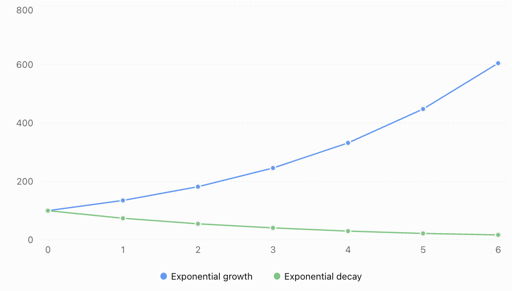
Both curves are exponential, but their behaviour is different.
For exponential growth, equal time intervals produce the same multiplication factor greater than one.
For exponential decay, equal time intervals produce the same multiplication factor between zero and one.
Radioactive Decay
Radioactive decay is the spontaneous transformation of an unstable atomic nucleus into a different nuclear state or another nucleus, often accompanied by the emission of radiation.
Examples of radioactive isotopes include carbon-14, iodine-131, uranium-238, and cobalt-60.
The decay of an individual nucleus is unpredictable. However, when a sample contains a very large number of radioactive nuclei, the expected number remaining follows a predictable exponential relationship.
The radioactive decay equation
Radioactive decay is commonly written as:
N(t) = N₀e⁻λᵗ
Where:
-
N(t) = expected number of undecayed radioactive nuclei at time t.
-
N₀ = initial number of radioactive nuclei.
-
λ = positive decay constant.
-
t = elapsed time.
The decay constant has units of inverse time, such as s⁻¹, day⁻¹, or year⁻¹.
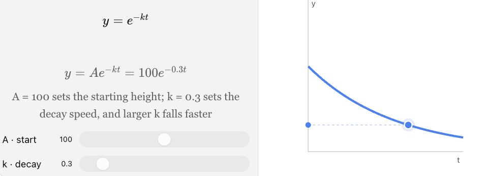
A larger decay constant means faster radioactive decay.
Visualising exponential decay
How the decay constant changes the curve
Half-Life
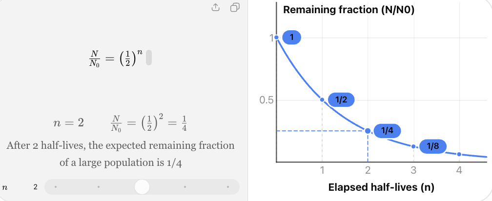
The half-life of a radioactive isotope is the time required for the expected number of undecayed nuclei in a large sample to decrease to half its original value.
After one half-life, 50% remains.
After two half-lives, 25% remains.
After three half-lives, 12.5% remains.
After four half-lives, 6.25% remains.
|
Number of half-lives |
Fraction remaining |
Percentage remaining |
|---|---|---|
|
0 |
1 |
100% |
|
1 |
1/2 |
50% |
|
2 |
1/4 |
25% |
|
3 |
1/8 |
12.5% |
|
4 |
1/16 |
6.25% |
|
5 |
1/32 |
3.125% |
The half-life formula
Half-life and decay constant are related by:
t½ = ln(2)/λ
Equivalently:
λ = ln(2)/t½
These equations allow us to calculate one quantity when the other is known.
Worked Example 1: Radioactive Material Remaining
A radioactive sample initially contains 160 g of a particular isotope.
Its half-life is 8 days.
Calculate the amount remaining after 24 days.
Step 1: Calculate the number of half-lives.
Number of half-lives = 24/8
Number of half-lives = 3
Step 2: Apply the half-life relationship.
Remaining mass = 160 × (1/2)³
Remaining mass = 160 × 1/8
Remaining mass = 20 g
After 24 days, the expected remaining mass of the original isotope is 20 g.
Worked Example 2: Finding the Decay Constant
An isotope has a half-life of 12 hours.
Calculate its decay constant.
Use:
λ = ln(2)/t½
Substitute:
λ = ln(2)/12
λ = 0.693147/12
λ ≈ 0.05776 h⁻¹
The exponential decay model is:
N(t) = N₀e⁻⁰·⁰⁵⁷⁷⁶ᵗ
where t is measured in hours.
Worked Example 3: Finding the Time Required for Decay
A radioactive sample follows:
M(t) = 500e⁻⁰·⁰⁸ᵗ
where M is measured in grams and t in years.
How long will it take for the sample to decrease to 100 g of the original isotope?
Step 1: Substitute the target mass.
100 = 500e⁻⁰·⁰⁸ᵗ
Step 2: Divide by 500.
0.2 = e⁻⁰·⁰⁸ᵗ
Step 3: Take natural logarithms.
ln(0.2) = −0.08t
Step 4: Solve.
t = ln(0.2)/(−0.08)
t ≈ −1.609438/(−0.08)
t ≈ 20.12 years
The sample reaches 100 g after approximately 20.12 years.
Radioactive Activity
The activity of a radioactive sample is the number of nuclear decays per unit time.
The SI unit of activity is the becquerel (Bq).
1 Bq = 1 decay per second
For a large sample:
A = λN
Where:
-
A = activity in Bq.
-
λ = decay constant in s⁻¹.
-
N = number of undecayed radioactive nuclei.
Because the number of radioactive nuclei decreases exponentially, activity also decreases exponentially:
A(t) = A₀e⁻λᵗ
Worked Example 4: Radioactive Activity
A sample initially has an activity of 800 Bq.
Its half-life is 5 hours.
Calculate its expected activity after 15 hours.
Number of half-lives:
15/5 = 3
Activity remaining:
A = 800 × (1/2)³
A = 800/8
A = 100 Bq
The expected activity after 15 hours is 100 Bq.
The activity and the number of undecayed nuclei have the same half-life.
Radiometric Dating
Radioactive decay can be used to estimate the age of certain materials.
Radiometric dating relies on measuring radioactive isotopes and interpreting how their quantities have changed over time.
One example is carbon-14 dating.
Carbon-14 is a radioactive isotope that is incorporated into living organisms through the carbon cycle.
After an organism dies, it generally stops exchanging carbon with its environment, and the carbon-14 already present continues to decay.
The half-life of carbon-14 is approximately 5,730 years.
Worked Example 5: Carbon-14 Dating
An archaeological sample contains 25% of the carbon-14 activity expected for a comparable modern sample.
Assume the sample has remained a closed system and the initial activity is appropriately estimated.
Estimate its age.
Step 1: Determine the remaining fraction.
25% = 0.25 = 1/4
Step 2: Express the fraction as powers of one-half.
1/4 = (1/2)²
Therefore, two half-lives have elapsed.
Step 3: Calculate the age.
Age = 2 × 5730
Estimated age = 11,460 years
In real radiocarbon dating, measured ages require calibration and may be affected by contamination, reservoir effects, and uncertainty in the initial carbon-14 activity.
The calculation above demonstrates the mathematical principle.
Interpreting Radioactive Decay Critically
Radioactive decay models are powerful because the decay constant is characteristic of a particular nuclear state under ordinary conditions.
However, several limitations must be recognised.
-
Radioactive decay is probabilistic at the level of individual nuclei.
-
The exponential law describes expected behaviour for large populations of nuclei.
-
Measuring instruments have uncertainties and background radiation.
-
Samples may contain mixtures of isotopes.
-
Radiometric dating requires assumptions about the original material and possible contamination.
The mathematics is reliable within the model, but scientific conclusions also depend on measurement quality and appropriate interpretation.
Chemical Concentration Scales
Chemists frequently work with extremely small or extremely large concentration ratios.
Logarithmic scales are useful because they compress large numerical ranges into manageable values.
One important example is the pH scale.
Understanding pH
pH is a logarithmic measure related to hydrogen ion activity in a solution.
The thermodynamic definition is:
pH = −log₁₀(aH⁺)
where aH⁺ is the dimensionless activity of hydrogen ions.
For many introductory calculations involving sufficiently dilute aqueous solutions, activity is approximated using molar concentration:
pH ≈ −log₁₀([H⁺]/(1 mol/L))
It is common in school-level chemistry to write the approximation as:
pH = −log₁₀[H⁺]
with [H⁺] understood to be the numerical concentration in mol/L under the dilute-solution approximation.
Why is pH logarithmic?
Hydrogen ion concentrations may vary by many orders of magnitude.
A logarithmic scale makes these differences easier to compare.
For example:
-
pH 2 corresponds approximately to [H⁺] = 10⁻² mol/L.
-
pH 3 corresponds approximately to [H⁺] = 10⁻³ mol/L.
-
pH 4 corresponds approximately to [H⁺] = 10⁻⁴ mol/L.
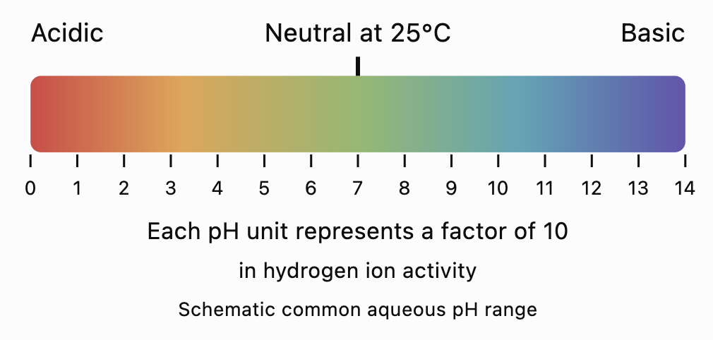
A decrease of one pH unit corresponds to a tenfold increase in hydrogen ion activity.
Understanding the pH scale
Worked Example 6: Calculating pH
A dilute aqueous solution has a hydrogen ion concentration of:
[H⁺] = 1 × 10⁻⁴ mol/L
Calculate its approximate pH.
Use:
pH ≈ −log₁₀(10⁻⁴)
Since log₁₀(10⁻⁴) = −4:
pH ≈ −(−4)
pH ≈ 4
The solution is acidic.
Worked Example 7: Finding Hydrogen Ion Concentration
A dilute aqueous solution has pH = 3.5.
Calculate its approximate hydrogen ion concentration.
Start with:
pH ≈ −log₁₀([H⁺])
Rearrange:
[H⁺] ≈ 10⁻ᵖᴴ mol/L
Substitute:
[H⁺] ≈ 10⁻³·⁵
[H⁺] ≈ 3.16 × 10⁻⁴ mol/L
Worked Example 8: Comparing Acidity
Solution A has pH 2.
Solution B has pH 5.
How many times greater is the hydrogen ion activity in Solution A?
The difference in pH is:
5 − 2 = 3
Each pH unit represents a factor of 10.
Therefore:
Ratio = 10³
Ratio = 1,000
Solution A has 1,000 times the hydrogen ion activity of Solution B.
This does not necessarily mean it contains 1,000 times the total amount of acid, because acid concentration, dissociation, and buffering also matter.
The pOH Scale
Another logarithmic chemical scale is pOH.
For dilute aqueous solutions:
pOH ≈ −log₁₀([OH⁻]/(1 mol/L))
At 25°C, for dilute aqueous solutions:
pH + pOH ≈ 14
Worked Example 9: Calculating pOH
A solution has pH = 9.2 at 25°C.
Calculate pOH.
pOH ≈ 14 − 9.2
pOH ≈ 4.8
The solution is basic.
At temperatures other than 25°C, the relationship changes because the ion product of water changes.
Other Logarithmic Scales in Science
Logarithms are useful wherever quantities span very large ranges.
Sound intensity level
Sound intensity level is measured in decibels.
β = 10log₁₀(I/I₀)
Where:
-
β = sound intensity level in decibels.
-
I = sound intensity.
-
I₀ = reference intensity.
For sound intensity in air, a commonly used reference is:
I₀ = 10⁻¹² W/m²
Worked Example 10: Comparing Sound Intensities
Two sounds have intensity levels of 60 dB and 80 dB.
Find the ratio of their intensities.
Difference:
80 − 60 = 20 dB
Using:
20 = 10log₁₀(I₂/I₁)
Divide by 10:
2 = log₁₀(I₂/I₁)
Convert to exponential form:
I₂/I₁ = 10²
I₂/I₁ = 100
The 80 dB sound has 100 times the physical intensity of the 60 dB sound, assuming the same reference intensity.
This does not mean it is perceived as 100 times as loud.
Why logarithmic scales are useful
A logarithmic scale converts multiplication into addition.
For example:
log₁₀(1000) = 3
log₁₀(10000) = 4
A tenfold increase produces an increase of one logarithmic unit.
This makes logarithmic scales particularly useful for quantities varying across many orders of magnitude.
Biological Growth Models
Living organisms reproduce, develop, compete for resources, and respond to their environment. Mathematical models help scientists investigate these processes.
Two particularly important biological models are exponential growth and logistic growth.
Exponential Population Growth
Exponential growth occurs when the instantaneous rate of population increase is proportional to the current population.
The model is:
P(t) = P₀eʳᵗ
Where:
-
P(t) = population at time t.
-
P₀ = initial population.
-
r = positive continuous growth constant.
-
t = time.
This model assumes that the relative growth rate remains constant.
Worked Example 11: Bacterial Growth
A bacterial culture initially contains 500 bacteria.
Under ideal laboratory conditions, the population grows continuously at a rate of 0.4 per hour.
Calculate the expected population after six hours.
Step 1: Write the model.
P(t) = 500e⁰·⁴ᵗ
Step 2: Substitute t = 6.
P(6) = 500e^(0.4 × 6)
P(6) = 500e²·⁴
Step 3: Evaluate.
e²·⁴ ≈ 11.02318
P(6) ≈ 500 × 11.02318
P(6) ≈ 5,512 bacteria
The model predicts approximately 5,512 bacteria after six hours.
This prediction assumes that nutrients, space, temperature, and other conditions remain suitable for continued growth.
Doubling Time in Biology
Doubling time describes how long a growing population takes to become twice its initial size.
For continuous exponential growth:
tᵈ = ln(2)/r
Where r > 0.
Worked Example 12: Calculating Bacterial Doubling Time
A bacterial population grows continuously at a rate of 0.35 per hour.
Calculate its doubling time.
tᵈ = ln(2)/0.35
tᵈ = 0.693147/0.35
tᵈ ≈ 1.98 hours
The population doubles approximately every 1.98 hours.
Interpreting the result
A constant doubling time means that the population multiplies by the same factor over equal time intervals.
However, the absolute increase becomes larger as the population grows.
For example, doubling from 100 to 200 adds 100 organisms.
Doubling from 10,000 to 20,000 adds 10,000 organisms.
The proportional change is the same, but the numerical increase is different.
Logistic Growth in Biology
Exponential growth cannot usually continue indefinitely in a limited environment.
As a population increases, resources become scarcer and competition becomes more significant.
A logistic model accounts for these limitations.
The standard logistic function is:
P(t) = K/(1 + Ae⁻ʳᵗ)
Where:
-
K = carrying capacity.
-
A = constant determined by the initial population.
-
r = intrinsic growth parameter.
-
t = time.
For an initial population P₀:
A = (K − P₀)/P₀
Comparing exponential and logistic growth
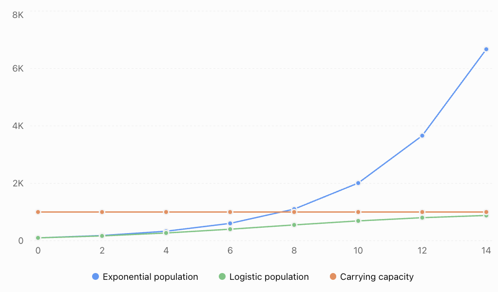
Both models begin with 100 organisms and use a growth parameter of 0.3 per hour. The logistic model includes a carrying capacity of 1,000.
The exponential model predicts continued rapid growth.
The logistic model predicts that growth slows as the population approaches carrying capacity.
Worked Example 13: Logistic Bacterial Growth
A bacterial culture begins with 200 organisms.
The carrying capacity of its environment is 5,000 organisms, and the intrinsic growth parameter is 0.5 per hour.
Calculate the expected population after eight hours.
Step 1: Calculate A.
A = (K − P₀)/P₀
A = (5000 − 200)/200
A = 4800/200
A = 24
Step 2: Write the model.
P(t) = 5000/(1 + 24e⁻⁰·⁵ᵗ)
Step 3: Substitute t = 8.
P(8) = 5000/(1 + 24e⁻⁴)
Step 4: Evaluate.
e⁻⁴ ≈ 0.0183156
P(8) ≈ 5000/[1 + 24(0.0183156)]
P(8) ≈ 5000/1.439575
P(8) ≈ 3,473 bacteria
The population is predicted to reach approximately 3,473 organisms after eight hours.
The model predicts that the population will gradually approach 5,000 rather than grow without limit.
Interpreting Carrying Capacity
Carrying capacity represents the population size that an environment can sustain under the conditions assumed by the model.
It may depend on:
-
Food and nutrient availability.
-
Water supply.
-
Available space.
-
Competition.
-
Waste accumulation.
-
Predation and disease.
-
Temperature and other environmental conditions.
Carrying capacity is not necessarily permanent.
A change in environmental conditions may increase or decrease the number of organisms that can be supported.
Other Scientific Exponential Applications
Exponential functions are not limited to radioactive decay and biological growth.
They also describe several important processes in chemistry, physics, and environmental science.
First-Order Chemical Reactions
In a first-order chemical reaction, the rate of disappearance of a reactant is proportional to its concentration.
For a reactant A:
d[A]/dt = −k[A]
The integrated rate law is:
A = [A]₀e⁻ᵏᵗ
Where:
-
A = reactant concentration at time t.
-
[A]₀ = initial concentration.
-
k = first-order rate constant.
-
t = time.
The mathematical form is the same as radioactive decay.
However, the underlying physical processes are different.
Radioactive decay involves nuclear transformations, while chemical reactions involve rearrangements of atoms and chemical bonds.
Worked Example 14: First-Order Reaction
A reactant has an initial concentration of 0.80 mol/L.
Its concentration follows first-order kinetics with k = 0.15 min⁻¹.
Calculate the concentration after 10 minutes.
A = 0.80e⁻⁰·¹⁵ᵗ
A = 0.80e⁻¹·⁵
Since e⁻¹·⁵ ≈ 0.223130:
A ≈ 0.80 × 0.223130
A ≈ 0.179 mol/L
The reactant concentration decreases to approximately 0.179 mol/L.
Newton's Law of Cooling
The rate at which an object cools is often approximately proportional to the temperature difference between the object and its surroundings.
For constant ambient temperature:
T(t) = Tₐ + (T₀ − Tₐ)e⁻ᵏᵗ
Where:
-
T(t) = object temperature at time t.
-
Tₐ = ambient temperature.
-
T₀ = initial object temperature.
-
k = positive cooling constant.
The temperature difference, T − Tₐ, decreases exponentially.
Worked Example 15: Cooling Coffee
A cup of coffee begins at 85°C in a room at 25°C.
The cooling constant is 0.08 min⁻¹.
Calculate the coffee's temperature after 15 minutes.
T(t) = 25 + (85 − 25)e⁻⁰·⁰⁸ᵗ
T(15) = 25 + 60e⁻¹·²
Since e⁻¹·² ≈ 0.301194:
T(15) ≈ 25 + 60(0.301194)
T(15) ≈ 25 + 18.0716
T(15) ≈ 43.07°C
The coffee is predicted to cool to approximately 43.1°C.
It approaches room temperature rather than approaching 0°C.
Light Absorption and Concentration
Another important scientific relationship is the Beer–Lambert law.
For a suitable solution:
A = εlc
Where:
-
A = absorbance.
-
ε = molar absorption coefficient.
-
l = optical path length.
-
c = concentration.
Absorbance is defined by:
A = log₁₀(I₀/I)
Where:
-
I₀ = incident light intensity.
-
I = transmitted light intensity.
Therefore:
I = I₀ × 10⁻ᴬ
Combining the relationships:
I = I₀ × 10⁻εˡᶜ
This means that transmitted light intensity decreases exponentially with concentration when ε and l are constant.
Worked Example 16: Absorbance
A solution has absorbance A = 0.60.
Calculate the fraction of incident light transmitted.
I/I₀ = 10⁻⁰·⁶⁰
I/I₀ ≈ 0.2512
Transmitted fraction ≈ 0.251
Approximately 25.1% of the incident light is transmitted.
This relationship is widely used in spectrophotometry to investigate chemical concentrations.
Interpreting Exponential Relationships Critically
Exponential models share a common mathematical form, but their parameters must be interpreted in context.
Consider three models:
Radioactive decay
N(t) = 1000e⁻⁰·²ᵗ
Bacterial growth
P(t) = 1000e⁰·²ᵗ
Chemical concentration
C(t) = 0.50e⁻⁰·²ᵗ
Although these equations use the same numerical magnitude for the exponential constant, they describe different quantities.
The meaning of the constant depends on the process and the units of time.
|
Model |
Initial quantity |
Constant |
Interpretation |
|---|---|---|---|
|
Radioactive decay |
1,000 nuclei |
−0.2 |
Expected number decreases |
|
Bacterial growth |
1,000 organisms |
+0.2 |
Population increases |
|
Chemical concentration |
0.50 mol/L |
−0.2 |
Concentration decreases |
A mathematical model must always be accompanied by clearly defined variables and units.
Estimating a Growth or Decay Constant from Data
Suppose a quantity follows:
Q(t) = Q₀eᵏᵗ
Taking natural logarithms gives:
ln[Q(t)/Q₀] = kt
Therefore:
k = ln[Q(t)/Q₀]/t
This formula works for both growth and decay.
For growth, k is positive.
For decay, k is negative.
Worked Example 17: Estimating a Decay Constant
A chemical concentration decreases from 0.60 mol/L to 0.24 mol/L in eight minutes.
Assume first-order decay.
Find the decay constant.
Step 1: Substitute the values.
k = ln(0.24/0.60)/8
k = ln(0.4)/8
Step 2: Evaluate.
ln(0.4) ≈ −0.916291
k ≈ −0.916291/8
k ≈ −0.11454 min⁻¹
The signed exponential constant is −0.11454 min⁻¹.
Equivalently, the positive first-order decay constant is:
λ ≈ 0.11454 min⁻¹
The concentration model becomes:
C(t) = 0.60e⁻⁰·¹¹⁴⁵⁴ᵗ
Using Logarithmic Transformations to Analyse Scientific Data
A useful property of exponential models is that taking logarithms converts them into linear relationships.
Starting with:
Q(t) = Q₀eᵏᵗ
Take natural logarithms:
ln[Q(t)] = ln(Q₀) + kt
This has the form:
y = mx + b
where:
-
y = ln[Q(t)]
-
x = t
-
slope = k
-
intercept = ln(Q₀)
Strictly, logarithms must be taken of dimensionless quantities, so a reference unit is understood when logarithms of measured quantities are used.
Why is this useful?
If experimental data follow an exponential model, plotting the natural logarithm of the measured quantity against time should produce an approximately straight line.
The slope can be used to estimate the growth or decay constant.
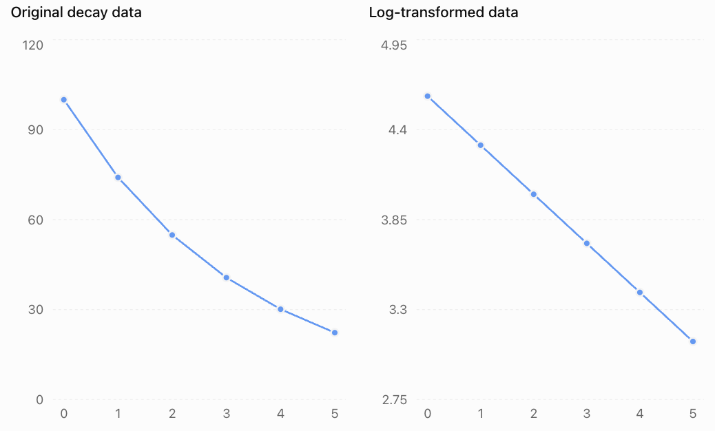
The original quantity decreases exponentially.
The logarithm of the quantity decreases linearly.
In this example, the slope of the transformed graph is approximately −0.3 per unit time.
This suggests a decay constant of 0.3 per unit time.
Important limitation
A straight line on a logarithmic transformation supports an exponential relationship, but it does not prove the underlying process is exponential.
Measurement errors, small datasets, and limited observation ranges can make different models appear similar.
Authentic Scientific Investigation: Evaluating a Bacterial Culture
A scientist grows bacteria in a nutrient solution and records the population.
|
Time (hours) |
Population |
|---|---|
|
0 |
200 |
|
2 |
365 |
|
4 |
665 |
|
6 |
1,211 |
|
8 |
2,207 |
The scientist wants to determine whether exponential growth is an appropriate model.
Step 1: Examine population ratios
For equal two-hour intervals:
365/200 ≈ 1.825
665/365 ≈ 1.822
1211/665 ≈ 1.821
2207/1211 ≈ 1.822
The ratios are approximately constant.
This supports an exponential model.
Step 2: Estimate the growth constant
Using the first and final measurements:
k = ln(2207/200)/8
k = ln(11.035)/8
k ≈ 0.300 per hour
Step 3: Construct the model
P(t) ≈ 200e⁰·³ᵗ
Step 4: Predict the population after 10 hours
P(10) ≈ 200e³
P(10) ≈ 200(20.0855)
P(10) ≈ 4,017 bacteria
Step 5: Evaluate the prediction
The model predicts approximately 4,017 bacteria after 10 hours.
However, the scientist should consider whether nutrients, oxygen, space, or waste accumulation may begin limiting growth.
If the culture approaches environmental carrying capacity, a logistic or other growth model may become more appropriate.
The exponential model is supported by the observed early data, but its long-term reliability has not been established.
Common Mistakes
Mistake 1: Confusing exponential growth and decay
A positive exponential constant represents growth, while a negative constant represents decay.
Correction: Check the sign of the exponent coefficient.
Mistake 2: Subtracting half the original quantity every half-life
After each half-life, half of the amount currently remaining is expected to survive.
Correction: Use repeated multiplication by 1/2.
Mistake 3: Confusing half-life and decay constant
Half-life has units of time, while the decay constant has units of inverse time.
Correction: Use t½ = ln(2)/λ.
Mistake 4: Treating radioactive decay as deterministic for individual atoms
The time at which a particular nucleus decays cannot generally be predicted.
Correction: Interpret exponential decay statistically for large populations of nuclei.
Mistake 5: Treating the pH scale as linear
A difference of one pH unit represents a factor of 10 in hydrogen ion activity, not a fixed additive change.
Correction: Use logarithmic relationships when comparing acidity.
Mistake 6: Confusing logarithms with natural logarithms
The pH scale uses base-10 logarithms, while continuous exponential models commonly use natural logarithms.
Correction: Identify the logarithm base required by the model.
Mistake 7: Ignoring units
A decay constant measured in hours⁻¹ cannot be used directly with time measured in days.
Correction: Convert quantities into consistent units.
Mistake 8: Assuming biological populations grow exponentially forever
Real populations are limited by resources and environmental conditions.
Correction: Evaluate whether a logistic or another resource-limited model is more appropriate.
Mistake 9: Assuming all exponential models describe the same process
Radioactive decay, chemical reactions, and biological growth may have similar equations but different mechanisms.
Correction: Interpret each model using the scientific context.
Mistake 10: Ignoring experimental uncertainty
Measurements contain error, and estimated model parameters may be uncertain.
Correction: Use multiple observations, examine residuals, and communicate limitations.
Key Terms
-
Exponential Growth: Growth in which the instantaneous rate of increase is proportional to the current quantity.
-
Exponential Decay: Decrease in which the instantaneous rate of decrease is proportional to the current quantity.
-
Radioactive Decay: Spontaneous transformation of an unstable atomic nucleus.
-
Half-Life: Time required for the expected remaining radioactive population to decrease by half.
-
Decay Constant: Positive parameter describing the rate of exponential decay.
-
Activity: Number of radioactive decays per unit time.
-
Becquerel (Bq): SI unit of radioactive activity, equal to one decay per second.
-
Radiometric Dating: Estimating the age of materials using radioactive isotope measurements.
-
Carbon-14 Dating: Radiometric dating method using the decay of carbon-14.
-
Hydrogen Ion Activity: Effective thermodynamic measure of hydrogen ions in solution.
-
pH: Logarithmic measure related to hydrogen ion activity.
-
pOH: Logarithmic measure related to hydroxide ion activity.
-
Logarithmic Scale: Scale representing multiplicative changes through additive differences.
-
Decibel: Logarithmic unit used to express ratios, including sound intensity levels.
-
First-Order Reaction: Reaction whose rate is proportional to the concentration of a particular reactant.
-
Rate Constant: Parameter relating a reaction rate to reactant concentrations.
-
Biological Growth: Increase in a biological population or another biological quantity.
-
Doubling Time: Time required for an exponentially growing quantity to double.
-
Logistic Growth: Growth that slows as a population approaches carrying capacity.
-
Carrying Capacity: Population size an environment can sustain under the assumed conditions.
-
Newton's Law of Cooling: Model relating the rate of temperature change to the difference between an object's temperature and its surroundings.
-
Beer–Lambert Law: Relationship connecting absorbance, optical path length, and concentration.
-
Logarithmic Transformation: Applying logarithms to data to simplify or investigate mathematical relationships.
-
Scientific Model: Mathematical or conceptual representation of a scientific process.
-
Model Limitation: A condition restricting the accuracy or applicability of a model.
Key Takeaways
-
Exponential models describe processes in which the rate of change is proportional to the current quantity.
-
Radioactive decay follows an exponential relationship in expectation for large samples.
-
Half-life and decay constant are connected by t½ = ln(2)/λ.
-
Radioactive activity decreases with the same decay constant as the number of undecayed nuclei.
-
Natural logarithms allow us to solve for unknown times and rate constants.
-
The pH scale is logarithmic, with each unit representing a factor of 10 in hydrogen ion activity.
-
Logarithmic scales help scientists represent quantities spanning large numerical ranges.
-
Biological populations may initially grow exponentially but later experience resource limitations.
-
Logistic models incorporate carrying capacity.
-
First-order chemical reactions and Newton's law of cooling also involve exponential relationships.
-
Logarithmic transformations can help identify exponential patterns in experimental data.
-
Scientific models must be interpreted using appropriate units, assumptions, and experimental evidence.
Check Your Understanding
Questions
Question 1: Exponential Growth and Decay
Determine whether each model represents growth or decay.
a) Q(t) = 500e⁰·²ᵗ
b) Q(t) = 800e⁻⁰·¹ᵗ
c) Q(t) = 100e⁰ᵗ
Question 2: Radioactive Half-Life
A radioactive sample initially contains 240 g of an isotope with a half-life of six years.
Calculate the expected amount remaining after 18 years.
Question 3: Decay Constant
An isotope has a half-life of 20 days.
Calculate its decay constant in day⁻¹.
Question 4: Radioactive Decay
A radioactive sample follows:
M(t) = 300e⁻⁰·⁰⁵ᵗ
Calculate the expected mass remaining after 10 years.
Question 5: Solving for Time
A radioactive sample follows:
N(t) = 1000e⁻⁰·⁰⁸ᵗ
How long will it take for the expected number of undecayed nuclei to decrease to 200?
Question 6: Radioactive Activity
A sample initially has an activity of 1,600 Bq and a half-life of four hours.
Calculate its expected activity after 12 hours.
Question 7: Carbon-14 Dating
An archaeological sample contains approximately 12.5% of its estimated original carbon-14 activity.
Using a half-life of 5,730 years, estimate its age.
Question 8: Calculating pH
A dilute aqueous solution has a hydrogen ion concentration of 1 × 10⁻⁵ mol/L.
Calculate its approximate pH.
Question 9: Hydrogen Ion Concentration
A dilute aqueous solution has pH 2.8.
Calculate its approximate hydrogen ion concentration.
Question 10: Comparing Acidity
Solution A has pH 3.
Solution B has pH 6.
How many times greater is the hydrogen ion activity in Solution A?
Question 11: Sound Intensity
Two sounds differ by 30 dB in sound intensity level.
Calculate the ratio of their physical intensities.
Question 12: Biological Growth
A bacterial population initially contains 400 organisms and grows continuously at 0.25 per hour.
Calculate the expected population after eight hours.
Question 13: Doubling Time
A bacterial population grows continuously at a rate of 0.4 per hour.
Calculate its doubling time.
Question 14: Logistic Growth
A population follows:
P(t) = 2000/(1 + 9e⁻⁰·³ᵗ)
a) Determine the carrying capacity.
b) Calculate the initial population.
c) Calculate the population after five years.
Question 15: First-Order Chemical Reaction
A reactant initially has a concentration of 0.50 mol/L.
Its concentration decreases according to first-order kinetics with k = 0.12 min⁻¹.
Calculate its concentration after 15 minutes.
Question 16: Scientific Modelling
A scientist observes that a bacterial population grows exponentially during the first six hours of an experiment.
Explain why the exponential model may become inaccurate after a much longer period.
Fully Worked Answers
Answer 1: Exponential Growth and Decay
a) The exponential constant is positive.
Exponential growth.
b) The exponential constant is negative.
Exponential decay.
c) The exponential constant is zero.
Since e⁰ = 1:
Q(t) = 100
The quantity remains constant.
Answer 2: Radioactive Half-Life
Initial mass = 240 g
Half-life = 6 years
Elapsed time = 18 years
Number of half-lives:
18/6 = 3
Remaining mass:
M = 240(1/2)³
M = 240/8
M = 30 g
Answer 3: Decay Constant
Use:
λ = ln(2)/t½
Substitute:
λ = 0.693147/20
λ ≈ 0.03466 day⁻¹
Answer 4: Radioactive Decay
Given:
M(t) = 300e⁻⁰·⁰⁵ᵗ
At t = 10:
M(10) = 300e⁻⁰·⁵
Since e⁻⁰·⁵ ≈ 0.606531:
M(10) ≈ 300 × 0.606531
M(10) ≈ 181.96 g
Answer 5: Solving for Time
Given:
N(t) = 1000e⁻⁰·⁰⁸ᵗ
Set N(t) = 200:
200 = 1000e⁻⁰·⁰⁸ᵗ
Divide by 1000:
0.2 = e⁻⁰·⁰⁸ᵗ
Take natural logarithms:
ln(0.2) = −0.08t
t = ln(0.2)/(−0.08)
t ≈ 20.12 time units
Answer 6: Radioactive Activity
Initial activity = 1600 Bq
Half-life = 4 hours
Elapsed time = 12 hours
Number of half-lives:
12/4 = 3
Activity:
A = 1600(1/2)³
A = 1600/8
A = 200 Bq
Answer 7: Carbon-14 Dating
Remaining activity = 12.5%
Convert to a fraction:
12.5% = 0.125 = 1/8
Since:
1/8 = (1/2)³
Three half-lives have elapsed.
Age:
3 × 5730
Estimated age = 17,190 years
This is an uncalibrated mathematical estimate.
Answer 8: Calculating pH
Given:
[H⁺] = 1 × 10⁻⁵ mol/L
Using the dilute-solution approximation:
pH ≈ −log₁₀(10⁻⁵)
pH ≈ −(−5)
pH ≈ 5
Answer 9: Hydrogen Ion Concentration
Given:
pH = 2.8
Use:
[H⁺] ≈ 10⁻ᵖᴴ mol/L
Substitute:
[H⁺] ≈ 10⁻²·⁸
[H⁺] ≈ 1.58 × 10⁻³ mol/L
Answer 10: Comparing Acidity
pH difference:
6 − 3 = 3
Hydrogen ion activity ratio:
10³ = 1000
Solution A has 1,000 times the hydrogen ion activity of Solution B.
Answer 11: Sound Intensity
Given a difference of 30 dB:
30 = 10log₁₀(I₂/I₁)
Divide by 10:
3 = log₁₀(I₂/I₁)
Convert to exponential form:
I₂/I₁ = 10³
Intensity ratio = 1,000
The higher-level sound has 1,000 times the physical intensity of the lower-level sound.
Answer 12: Biological Growth
Given:
P₀ = 400
r = 0.25 h⁻¹
t = 8 hours
Model:
P(t) = 400e⁰·²⁵ᵗ
Substitute:
P(8) = 400e²
Since e² ≈ 7.389056:
P(8) ≈ 400 × 7.389056
P(8) ≈ 2,956 organisms
Answer 13: Doubling Time
Use:
tᵈ = ln(2)/r
Substitute:
tᵈ = 0.693147/0.4
tᵈ ≈ 1.73 hours
Answer 14: Logistic Growth
Given:
P(t) = 2000/(1 + 9e⁻⁰·³ᵗ)
Part a: Carrying capacity
The numerator gives:
K = 2000
Part b: Initial population
At t = 0:
P(0) = 2000/(1 + 9e⁰)
P(0) = 2000/10
P₀ = 200
Part c: Population after five years
P(5) = 2000/(1 + 9e⁻¹·⁵)
Since e⁻¹·⁵ ≈ 0.223130:
P(5) ≈ 2000/[1 + 9(0.223130)]
P(5) ≈ 2000/3.00817
P(5) ≈ 665 organisms
Answer 15: First-Order Chemical Reaction
Initial concentration = 0.50 mol/L
k = 0.12 min⁻¹
t = 15 minutes
Model:
A = 0.50e⁻⁰·¹²ᵗ
Substitute:
A = 0.50e⁻¹·⁸
Since e⁻¹·⁸ ≈ 0.165299:
A ≈ 0.50 × 0.165299
A ≈ 0.08265 mol/L
Answer 16: Scientific Modelling
Exponential growth assumes that the relative growth rate remains constant.
During the early stages of bacterial growth, nutrients and space may be plentiful.
As the population increases, however, nutrients may become depleted, waste products may accumulate, and competition may increase.
These changes can reduce the growth rate.
Therefore, an exponential model that fits the first six hours may overestimate the population over a longer period.
A logistic or another resource-limited growth model may become more appropriate.
Final Reflection
Exponential and logarithmic relationships provide a powerful mathematical framework for understanding scientific change.
Radioactive decay, first-order chemical reactions, and some cooling processes involve quantities that decrease exponentially. Biological populations may grow exponentially under favourable conditions, while logistic models describe how environmental limitations can slow growth.
Logarithmic scales, such as pH and decibels, allow scientists to interpret quantities spanning enormous ranges of values.
The most important general exponential relationship is:
Q(t) = Q₀eᵏᵗ
However, the meaning of this equation depends on the scientific process being studied.
A successful scientific model combines mathematical accuracy with scientific understanding. It explains observed patterns, supports predictions, and recognises the assumptions and limitations that determine when those predictions are reliable.
3. Exponential Models in Technology
Learning outcomes
- I can explain exponential growth in computing.
- I can analyse information growth.
- I can recognise exponential trends in technology.
- I can interpret technological data.
- I can solve technology-based applications.
Introduction
Technology develops through processes that can produce rapid and sometimes surprising changes. Computing power, data storage, network activity, digital information, and the number of connected devices have all experienced periods of substantial growth.
One of the most important mathematical tools for understanding these changes is the exponential function.
Consider a computer system whose processing capacity doubles every two years. Initially, the increase may appear modest. However, repeated doubling produces increasingly large changes.
A system with an initial capacity of 100 units would develop as follows:
|
Time (years) |
Processing capacity |
|---|---|
|
0 |
100 |
|
2 |
200 |
|
4 |
400 |
|
6 |
800 |
|
8 |
1,600 |
|
10 |
3,200 |
After ten years, the capacity has increased by a factor of 32.
This is not linear growth. The capacity does not increase by the same amount every two years. Instead, it multiplies by the same factor.
Exponential models help us investigate technological growth, estimate future requirements, compare development trends, and understand why seemingly small percentage changes can produce enormous long-term effects.
However, exponential growth cannot continue indefinitely in every technological system. Physical limitations, economic constraints, market saturation, and changes in technology can alter growth patterns.
In this lesson, we will explore exponential growth in computing, digital information, data storage, network systems, and other technological applications. We will also learn to interpret technological data critically and evaluate the limitations of exponential models.
Understanding Exponential Growth
An exponential relationship occurs when a quantity changes by a constant percentage or multiplication factor over equal intervals.
The general discrete exponential model is:
Q(t) = Q₀bᵗ
Where:
-
Q(t) = quantity after time t.
-
Q₀ = initial quantity.
-
b = multiplication factor per time unit.
-
t = elapsed time.
If b > 1, the model represents exponential growth.
If 0 < b < 1, the model represents exponential decay.
For continuous exponential growth, we use:
Q(t) = Q₀eᵏᵗ
Where:
-
e ≈ 2.71828.
-
k = continuous growth constant.
Comparing linear and exponential growth
Suppose two computer systems begin with a processing capacity of 100 units.
System A increases by 100 units every two years.
System B doubles every two years.
|
Time (years) |
Linear model |
Exponential model |
|---|---|---|
|
0 |
100 |
100 |
|
2 |
200 |
200 |
|
4 |
300 |
400 |
|
6 |
400 |
800 |
|
8 |
500 |
1,600 |
|
10 |
600 |
3,200 |
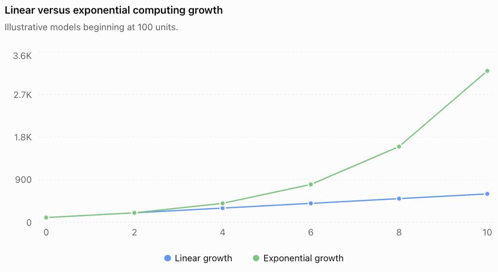
The linear model increases at a constant absolute rate.
The exponential model increases at a constant proportional rate.
This difference becomes especially important over long periods.
Exponential Growth in Computing
Computing technology has experienced periods of rapid improvements in processing capability, memory capacity, and component density.
Exponential models can describe these trends over suitable time intervals.
Moore's Law
One of the best-known historical observations in computing is Moore's law.
Moore's Law describes a historical trend in which the number of transistors on an integrated circuit increased approximately exponentially over time.
The commonly cited later formulation describes transistor counts doubling approximately every two years.
It is important to recognise that Moore's Law is an empirical technological observation, not a physical law guaranteeing future exponential growth.
Transistor density, processing speed, energy efficiency, and computing performance are related but distinct quantities. They do not necessarily increase at the same rate.
A simplified transistor growth model
Suppose a computer chip initially contains 2 million transistors, and the number doubles every two years.
The model is:
N(t) = 2,000,000 × 2^(t/2)
where t is measured in years.
Worked Example 1: Transistor Growth
Estimate the transistor count after eight years.
Step 1: Write the model.
N(t) = 2,000,000 × 2^(t/2)
Step 2: Substitute t = 8.
N(8) = 2,000,000 × 2^(8/2)
N(8) = 2,000,000 × 2⁴
Step 3: Evaluate.
N(8) = 2,000,000 × 16
N(8) = 32,000,000 transistors
The model predicts 32 million transistors after eight years.
Interpreting the result
The model predicts that the transistor count increases by a factor of 16 over eight years.
It does not establish that a chip with 16 times as many transistors is 16 times faster.
Actual performance depends on architecture, memory systems, clock speed, software, power constraints, and many other factors.
Doubling Time
Doubling time is particularly useful when analysing technological growth.
If a quantity doubles every T time units:
Q(t) = Q₀ × 2^(t/T)
Where:
-
Q₀ = initial quantity.
-
T = doubling time.
-
t = elapsed time.
Worked Example 2: Data Storage Capacity
A storage technology has a capacity of 500 GB and follows a hypothetical model in which capacity doubles every three years.
Calculate the capacity after 12 years.
Q(t) = 500 × 2^(t/3)
Substitute:
Q(12) = 500 × 2⁴
Q(12) = 500 × 16
Q(12) = 8,000 GB
Using decimal storage units:
8,000 GB = 8 TB
The predicted capacity after 12 years is 8 TB.
This is a mathematical projection, not a guarantee about future storage products.
Continuous Growth and Doubling Time
For a continuous exponential model:
Q(t) = Q₀eᵏᵗ
The doubling time is:
T = ln(2)/k
Equivalently:
k = ln(2)/T
Worked Example 3: Calculating a Growth Constant
A hypothetical computing capability doubles every 18 months.
Calculate the continuous growth constant in year⁻¹.
Convert the doubling time:
18 months = 1.5 years
Use:
k = ln(2)/1.5
k ≈ 0.693147/1.5
k ≈ 0.4621 year⁻¹
The model can be written as:
Q(t) = Q₀e⁰·⁴⁶²¹ᵗ
where t is measured in years.
The continuous growth constant is not the same as the effective annual percentage increase.
The effective annual growth factor is:
e⁰·⁴⁶²¹ ≈ 1.5874
Therefore, the effective annual increase is approximately:
58.74% per year
Analysing Information Growth
The amount of digital information stored, transmitted, and processed can increase rapidly.
Examples include:
-
Scientific datasets.
-
Digital photographs and videos.
-
Cloud storage.
-
Sensor measurements.
-
Internet traffic.
-
Business transaction records.
-
Machine-learning training data.
Not every form of digital information grows exponentially, and growth rates can change substantially over time.
However, exponential models are useful when data volumes increase by approximately constant percentages over equal periods.
Worked Example 4: Digital Information Growth
A research laboratory stores 12 TB of data.
Its stored data volume increases by 30% per year.
Assume this rate remains constant for five years.
The model is:
D(t) = 12(1.30)ᵗ
Calculate the amount of stored data after five years.
D(5) = 12(1.30)⁵
Since:
(1.30)⁵ = 3.71293
D(5) = 12 × 3.71293
D(5) ≈ 44.56 TB
The laboratory would need approximately 44.56 TB of storage after five years under the model.
Interpreting the result
The initial storage requirement is 12 TB.
After five years, the model predicts approximately 44.56 TB.
The required capacity increases by approximately 32.56 TB.
This illustrates why organisations must plan for future storage requirements rather than considering only their current needs.
Comparing Storage Growth Rates
Suppose two organisations begin with 10 TB of data.
Organisation A experiences 15% annual growth.
Organisation B experiences 30% annual growth.
Their models are:
A(t) = 10(1.15)ᵗ
B(t) = 10(1.30)ᵗ
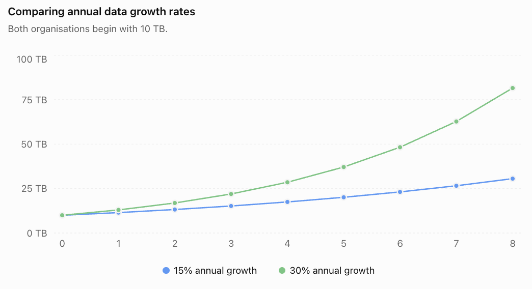
After eight years:
Organisation A requires approximately 30.59 TB.
Organisation B requires approximately 81.57 TB.
Although the growth rates differ by only 15 percentage points, the long-term storage requirements differ substantially.
This is a central feature of exponential growth.
Recognising Exponential Trends in Technological Data
A technological trend should not be described as exponential simply because its graph curves upward.
To identify exponential growth, we should examine the mathematical relationship between successive observations.
Constant differences versus constant ratios
For equally spaced time intervals:
-
Linear growth produces constant first differences.
-
Exponential growth produces constant ratios.
Consider two datasets.
|
Year |
Dataset A |
Dataset B |
|---|---|---|
|
0 |
100 |
100 |
|
1 |
150 |
150 |
|
2 |
200 |
225 |
|
3 |
250 |
337.5 |
|
4 |
300 |
506.25 |
For Dataset A, the first differences are:
50, 50, 50, 50
This suggests a linear model:
A(t) = 100 + 50t
For Dataset B, the successive ratios are:
150/100 = 1.5
225/150 = 1.5
337.5/225 = 1.5
506.25/337.5 = 1.5
This suggests an exponential model:
B(t) = 100(1.5)ᵗ
Worked Example 5: Identifying a Technology Trend
A technology company records the following hypothetical number of users for a new digital service.
|
Month |
Users |
|---|---|
|
0 |
2,000 |
|
1 |
2,400 |
|
2 |
2,880 |
|
3 |
3,456 |
|
4 |
4,147 |
Determine an appropriate model.
Step 1: Calculate successive ratios.
2400/2000 = 1.2
2880/2400 = 1.2
3456/2880 = 1.2
4147/3456 ≈ 1.200
The ratios are approximately constant.
Step 2: Identify the growth factor.
Growth factor = 1.2
Monthly growth rate = 20%
Step 3: Construct the model.
U(t) = 2000(1.2)ᵗ
where t is measured in months.
Step 4: Predict the number of users after six months.
U(6) = 2000(1.2)⁶
U(6) ≈ 2000(2.985984)
U(6) ≈ 5,972 users
The model predicts approximately 5,972 users after six months.
The prediction assumes the same growth pattern continues.
Interpreting Growth Rates
A growth factor and a percentage growth rate are related by:
b = 1 + r
where r is expressed as a decimal.
Therefore:
r = b − 1
For example:
-
b = 1.05 means 5% growth per period.
-
b = 1.20 means 20% growth per period.
-
b = 1.50 means 50% growth per period.
-
b = 2.00 means 100% growth per period, or doubling.
A 20% increase each year does not mean the quantity doubles every five years.
Repeated percentage growth compounds.
Worked Example 6: Finding the Doubling Time
A digital platform's data volume grows by 25% per year.
How long will it take for the data volume to double?
The model is:
D(t) = D₀(1.25)ᵗ
Set D(t) = 2D₀:
2D₀ = D₀(1.25)ᵗ
Divide by D₀:
2 = (1.25)ᵗ
Take natural logarithms:
ln(2) = t ln(1.25)
Therefore:
t = ln(2)/ln(1.25)
t ≈ 3.11 years
The data volume doubles after approximately 3.11 years under the model.
Logarithmic Graphs and Technological Trends
Exponential growth can be difficult to interpret when quantities become very large.
A logarithmic scale helps scientists and engineers compare values across several orders of magnitude.
Suppose:
Q(t) = Q₀eᵏᵗ
Taking natural logarithms gives:
ln[Q(t)] = ln(Q₀) + kt
This is a linear relationship.
Therefore, a plot of ln(Q) against time produces a straight line when the data follow an exact exponential model.
Strictly, logarithms are applied to dimensionless numerical ratios, so a reference unit is understood when working with measured quantities.
Example: Logarithmic Transformation
Suppose computing capacity follows:
C(t) = 100e⁰·⁴ᵗ
Then:
ln[C(t)] = ln(100) + 0.4t
Since ln(100) ≈ 4.6052:
ln[C(t)] ≈ 4.6052 + 0.4t
The transformed relationship has:
-
Slope = 0.4 per year.
-
Vertical intercept ≈ 4.6052.
The slope represents the continuous growth constant.
Why this matters
Logarithmic transformations can help researchers:
-
Identify approximately exponential patterns.
-
Estimate growth constants.
-
Compare technologies with different initial capacities.
-
Detect changes in growth rates.
-
Investigate whether a trend is slowing or accelerating.
However, a straight line on a logarithmic plot does not prove that growth will continue indefinitely.
Compound Annual Growth Rate
Technological data are often reported using the compound annual growth rate (CAGR).
CAGR describes the constant annual growth rate that would produce the same overall change between two values.
The formula is:
CAGR = (Final value/Initial value)^(1/n) − 1
where n is the number of years.
Worked Example 7: Computing Capacity Growth
A hypothetical computing system increases in capacity from 2,000 units to 12,000 units over six years.
Calculate the compound annual growth rate.
CAGR = (12000/2000)^(1/6) − 1
CAGR = 6^(1/6) − 1
CAGR ≈ 0.347
CAGR ≈ 34.7% per year
This means the capacity experienced the same overall increase as a system growing by approximately 34.7% every year.
It does not mean the actual growth rate was identical each year.
Exponential Growth in Network Technology
Digital networks can experience rapid increases in users, devices, connections, and data traffic.
Examples include communication networks, cloud services, and connected sensor systems.
Worked Example 8: Network Traffic
A network carries 800 GB of data per day.
Traffic increases by 18% per year.
Assume this growth continues for five years.
The model is:
T(t) = 800(1.18)ᵗ
Calculate daily traffic after five years.
T(5) = 800(1.18)⁵
Since (1.18)⁵ ≈ 2.28776:
T(5) ≈ 800 × 2.28776
T(5) ≈ 1,830 GB per day
The model predicts daily traffic of approximately 1.83 TB after five years, using decimal storage units.
Planning for technological infrastructure
An organisation must ensure that its systems can handle future demand.
If traffic grows exponentially while network capacity remains fixed, the system may eventually become overloaded.
Mathematical models can help estimate when additional infrastructure will be needed.
Worked Example 9: When Will Capacity Be Exceeded?
A network currently carries 500 GB of traffic per day.
Traffic grows by 20% per year.
The network has a maximum capacity of 1,500 GB per day.
How long will it take for predicted demand to reach capacity?
Step 1: Write the model.
T(t) = 500(1.2)ᵗ
Step 2: Set traffic equal to capacity.
1500 = 500(1.2)ᵗ
Step 3: Divide by 500.
3 = (1.2)ᵗ
Step 4: Take logarithms.
ln(3) = t ln(1.2)
Step 5: Solve.
t = ln(3)/ln(1.2)
t ≈ 6.03 years
The model predicts that demand reaches the network's stated capacity after approximately 6.03 years.
If infrastructure upgrades can only be completed at the end of each year, the network would exceed capacity during the seventh year.
In practice, engineers would normally plan upgrades before full capacity is reached to maintain reliability and allow for unexpected traffic peaks.
Exponential Growth in Computer Algorithms
Exponential functions also appear in computing when analysing how the resources required by an algorithm increase with problem size.
This is an important distinction:
Exponential technological improvement is not the same as exponential computational complexity.
An exponential-time algorithm may become dramatically slower as the input size increases.
Example: Exponential Time Complexity
Suppose an algorithm requires approximately:
T = 2ⁿ operations
where n is the number of input elements.
|
Input size n |
Number of operations |
|---|---|
|
5 |
32 |
|
10 |
1,024 |
|
15 |
32,768 |
|
20 |
1,048,576 |
|
25 |
33,554,432 |
|
30 |
1,073,741,824 |
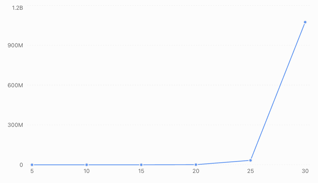
The number of operations doubles whenever the input size increases by one.
This means that even a relatively small increase in input size can cause a very large increase in computational work.
Worked Example 10: Algorithm Processing Time
An algorithm requires 2ⁿ operations.
A computer performs 1 million operations per second.
Estimate the processing time for n = 30.
Step 1: Calculate the number of operations.
T(30) = 2³⁰
T(30) = 1,073,741,824 operations
Step 2: Divide by processing speed.
Time = 1,073,741,824/1,000,000
Time ≈ 1,073.74 seconds
Step 3: Convert to minutes.
Time ≈ 1073.74/60
Time ≈ 17.90 minutes
Now consider n = 40.
T(40) = 2⁴⁰
T(40) = 1,099,511,627,776 operations
Processing time:
1,099,511,627,776/1,000,000 ≈ 1,099,512 seconds
This is approximately:
12.73 days
Increasing the input size from 30 to 40 increases the processing time by a factor of:
2¹⁰ = 1,024
This illustrates why algorithm efficiency is often more important than hardware improvements alone.
Comparing Technological Growth Models
Not every technological relationship is exponential.
Different processes require different mathematical models.
|
Model |
General form |
Possible technology application |
|---|---|---|
|
Linear |
y = mx + b |
Fixed monthly data additions |
|
Quadratic |
y = ax² + bx + c |
Certain computational workloads or cost relationships |
|
Exponential |
y = Abᵗ |
Constant-percentage data growth |
|
Logarithmic |
y = a ln(x) + b |
Some diminishing-return performance relationships |
|
Logistic |
y = K/(1 + Ae⁻ʳᵗ) |
Adoption approaching a finite market size |
Technology adoption and logistic growth
A new technology may initially attract only a small number of users.
As awareness increases, adoption can accelerate.
Eventually, growth may slow as the available market becomes saturated.
This pattern can sometimes be modelled by a logistic function.
Worked Example 11: Technology Adoption
A digital service follows the hypothetical model:
U(t) = 100000/(1 + 19e⁻⁰·⁵ᵗ)
where U(t) is the number of users and t is measured in years.
Calculate the initial number of users and the predicted number after eight years.
Step 1: Calculate the initial users.
At t = 0:
U(0) = 100000/(1 + 19e⁰)
U(0) = 100000/20
U(0) = 5,000 users
Step 2: Calculate users after eight years.
U(8) = 100000/(1 + 19e⁻⁴)
Since e⁻⁴ ≈ 0.0183156:
U(8) ≈ 100000/[1 + 19(0.0183156)]
U(8) ≈ 100000/1.347997
U(8) ≈ 74,184 users
The model predicts approximately 74,184 users after eight years.
The limiting value is 100,000 users.
Why logistic growth may be more realistic
A service cannot acquire more users than the available market allows under a fixed-market assumption.
Exponential growth may describe the early stages of adoption, but it eventually becomes unrealistic if the potential user population is limited.
The logistic model accounts for this constraint.
However, real markets can expand, competitors can enter, and adoption can decline, so the limiting value may change.
Interpreting Technological Data Critically
Exponential models are powerful, but they can be misleading when used without considering the underlying assumptions.
Historical trends do not guarantee future growth
A technology may grow exponentially for several years and then slow because of physical, economic, or practical limitations.
For example, transistor miniaturisation faces challenges involving heat, power consumption, manufacturing complexity, and cost.
Percentage growth can be misleading
A company increasing from 100 to 200 users experiences 100% growth.
A company increasing from 1 million to 1.1 million users experiences 10% growth.
The second company gains far more users, even though its percentage growth is much smaller.
Large numbers need appropriate units
Technological quantities may be expressed in:
-
Kilobytes, megabytes, gigabytes, terabytes, and petabytes.
-
Operations per second.
-
Bits per second.
-
Number of transistors.
-
Number of users or devices.
Always check whether units use decimal or binary prefixes.
For example:
1 TB = 1,000 GB
1 TiB = 1,024 GiB
These are different unit conventions.
Correlation does not establish causation
Two technological trends may increase together without one directly causing the other.
For example, computing capacity and global data volume may both increase over time.
However, their relationship may involve many interacting factors, including demand, software development, storage costs, and network infrastructure.
Evaluating Model Accuracy
A mathematical model should be evaluated using observed data.
A residual is:
Residual = Observed value − Predicted value
Consider a model predicting the number of users of a technology platform.
|
Year |
Observed users |
Predicted users |
Residual |
|---|---|---|---|
|
1 |
1,200 |
1,150 |
+50 |
|
2 |
1,500 |
1,550 |
−50 |
|
3 |
2,100 |
2,000 |
+100 |
|
4 |
2,500 |
2,650 |
−150 |
The residuals help identify how accurately the model represents the observations.
A systematic pattern in the residuals may indicate that the model is missing an important feature of the data.
Overfitting and extrapolation
A model may fit historical data extremely well but perform poorly when predicting future technological developments.
This can occur when:
-
The model is unnecessarily complicated.
-
Growth rates change.
-
The market becomes saturated.
-
New technologies replace older ones.
-
Unexpected economic or regulatory changes occur.
Predictions far beyond the observed time interval are especially uncertain.
Authentic Application: Planning Data Centre Capacity
A technology company currently stores 50 TB of information.
Its data volume has been increasing by approximately 28% per year.
The company wants to estimate future storage requirements.
Part A: Construct a model
Initial storage:
D₀ = 50 TB
Growth factor:
b = 1.28
Therefore:
D(t) = 50(1.28)ᵗ
where t is measured in years.
Part B: Predict storage after five years
D(5) = 50(1.28)⁵
Since:
(1.28)⁵ ≈ 3.435974
D(5) ≈ 50 × 3.435974
D(5) ≈ 171.80 TB
The company should expect approximately 171.8 TB of stored data after five years if the assumed growth rate continues.
Part C: Determine when storage reaches 200 TB
Set:
200 = 50(1.28)ᵗ
Divide by 50:
4 = (1.28)ᵗ
Take natural logarithms:
ln(4) = t ln(1.28)
Therefore:
t = ln(4)/ln(1.28)
t ≈ 5.61 years
The model predicts that the company's stored data will reach 200 TB after approximately 5.61 years.
Part D: Evaluate the model
The company should not assume the 28% growth rate will remain constant indefinitely.
Future storage requirements may be affected by:
-
Data compression.
-
Data retention policies.
-
Changes in customer demand.
-
More efficient software.
-
New products and services.
-
Regulations governing data storage.
-
Changes in the cost of storage.
The exponential model provides a useful planning estimate, but the company should regularly update it using new measurements.
Common Mistakes
Mistake 1: Assuming all technological growth is exponential
Some technologies grow linearly, while others follow logistic or irregular patterns.
Correction: Examine the data before selecting a model.
Mistake 2: Confusing constant increases with constant percentage growth
Adding 100 units per year is linear growth.
Increasing by 20% per year is exponential growth.
Correction: Compare differences and ratios.
Mistake 3: Confusing doubling time with growth rate
Doubling every two years does not mean increasing by 50% annually.
Correction: Use exponential equations to calculate the equivalent growth rate.
Mistake 4: Assuming Moore's Law guarantees future computing improvements
Moore's Law describes a historical technological trend, not a guaranteed physical relationship.
Correction: Consider engineering constraints and changing technological conditions.
Mistake 5: Assuming transistor count and computing performance are identical
More transistors do not automatically produce proportional improvements in processing speed.
Correction: Distinguish hardware component counts from actual performance measurements.
Mistake 6: Ignoring units
Confusing GB and TB, or months and years, can produce large errors.
Correction: Convert units before substituting values.
Mistake 7: Using percentages incorrectly
A growth rate of 15% corresponds to a multiplication factor of 1.15, not 0.15.
Correction: Use b = 1 + r.
Mistake 8: Extrapolating too far
An exponential model may produce unrealistic predictions over long periods.
Correction: State the time interval over which the model is reasonably supported.
Mistake 9: Confusing exponential technology improvement with exponential algorithm complexity
Exponential hardware improvements may be beneficial, while exponential algorithm complexity can make problems increasingly difficult.
Correction: Interpret the quantity represented by the exponential function.
Mistake 10: Ignoring physical and economic limitations
Storage, energy, manufacturing capacity, and market size can limit technological growth.
Correction: Consider alternative models when growth begins to slow.
Key Terms
-
Exponential Growth: Growth involving a constant proportional increase over equal intervals.
-
Growth Factor: Multiplier applied during each time interval.
-
Growth Rate: Percentage or proportional increase over a specified interval.
-
Doubling Time: Time required for a quantity to become twice its original value.
-
Continuous Growth Constant: Parameter describing exponential growth in the model Q(t) = Q₀eᵏᵗ.
-
Moore's Law: Historical observation concerning approximately exponential increases in transistor counts on integrated circuits.
-
Transistor: Semiconductor component used in electronic circuits.
-
Processing Capacity: Measure of the computational work a system can perform.
-
Digital Information: Information represented in digital form.
-
Data Storage: Retention of digital information.
-
Network Traffic: Data transmitted through a network over a specified period.
-
Bandwidth: Capacity of a communication channel to transmit data.
-
Algorithm: Step-by-step computational procedure for solving a problem.
-
Time Complexity: Description of how computational work grows with input size.
-
Exponential Complexity: Computational growth proportional to a function such as 2ⁿ.
-
Compound Annual Growth Rate (CAGR): Equivalent constant annual rate describing an overall change.
-
Logarithmic Scale: Scale that represents multiplicative changes using additive differences.
-
Logarithmic Transformation: Applying logarithms to data to investigate relationships.
-
Technology Adoption: Process by which users or organisations begin using a technology.
-
Logistic Growth: Growth that approaches a limiting value.
-
Market Saturation: Situation in which most potential users or customers have adopted a product or service.
-
Residual: Difference between an observed and predicted value.
-
Extrapolation: Prediction beyond the observed data range.
-
Model Limitation: Restriction on the validity or reliability of a mathematical model.
Key Takeaways
-
Exponential models describe quantities that increase by a constant percentage or multiplication factor.
-
Doubling produces increasingly large absolute changes.
-
Moore's Law describes a historical trend in transistor counts, not a guaranteed future law of computing performance.
-
Digital storage and information growth can sometimes be modelled exponentially.
-
Constant ratios in equally spaced data suggest exponential growth.
-
Natural logarithms allow us to calculate growth constants, doubling times, and when capacity thresholds will be reached.
-
Logarithmic transformations can help reveal exponential trends.
-
Network capacity planning is an important application of exponential models.
-
Exponential algorithm complexity describes rapidly increasing computational requirements.
-
Logistic models may be more appropriate when technology adoption approaches a limited market size.
-
Historical technological growth does not guarantee future exponential growth.
-
Reliable modelling requires appropriate units, accurate data, and careful evaluation of assumptions.
Check Your Understanding
Questions
Question 1: Identifying Exponential Growth
Determine which of the following represent exponential growth.
a) A computer's capacity increases by 200 units each year.
b) A data centre's storage requirement increases by 15% each year.
c) A server's workload doubles every four months.
d) A company's number of employees increases by 20 each year.
Question 2: Computing Capacity
A hypothetical computing system begins with a capacity of 500 units and doubles every two years.
Calculate its capacity after eight years.
Question 3: Data Growth
A research organisation stores 20 TB of data.
Its stored data increases by 25% annually.
Calculate the amount after four years.
Question 4: Growth Factor
A digital service increases its number of users by 18% each month.
Determine the monthly growth factor and write a model if the initial number of users is 3,000.
Question 5: Doubling Time
A technology's capacity doubles every three years.
Write an exponential model if its initial capacity is 1,200 units.
Question 6: Continuous Growth
A computing capability follows:
C(t) = 800e⁰·³ᵗ
Calculate its value after five years.
Question 7: Growth Constant
A technology doubles in capacity every 2.5 years.
Calculate its continuous growth constant.
Question 8: Identifying a Trend
A technology company records the following data.
|
Year |
Capacity |
|---|---|
|
0 |
100 |
|
1 |
140 |
|
2 |
196 |
|
3 |
274.4 |
Determine whether a linear or exponential model is more appropriate and explain why.
Question 9: CAGR
A digital platform increases from 5,000 users to 20,000 users over five years.
Calculate its compound annual growth rate.
Question 10: Network Capacity
A network currently carries 600 GB of traffic per day.
Traffic grows by 20% annually.
Calculate the predicted daily traffic after six years.
Question 11: Reaching a Threshold
A company's data storage requirement is 40 TB and increases by 30% per year.
How long will it take to reach 100 TB?
Question 12: Algorithm Complexity
An algorithm requires 2ⁿ operations.
Calculate the number of operations for n = 15 and n = 20.
By what factor does the number of operations increase?
Question 13: Technology Adoption
A service follows:
U(t) = 50000/(1 + 9e⁻⁰·⁴ᵗ)
Determine the limiting number of users and the initial number of users.
Question 14: Interpreting Moore's Law
Explain why a doubling in transistor count does not necessarily mean a doubling in computer processing speed.
Question 15: Critical Modelling
A company's stored data has increased by 40% annually for three years.
Explain why using the same growth rate to predict storage requirements 30 years into the future may be unreliable.
Fully Worked Answers
Answer 1: Identifying Exponential Growth
a) Linear — the capacity increases by a fixed amount.
b) Exponential — the storage requirement increases by a constant percentage.
c) Exponential — the workload doubles over equal time intervals.
d) Linear — the number of employees increases by a fixed amount.
Answer 2: Computing Capacity
Initial capacity = 500 units
Doubling time = 2 years
Elapsed time = 8 years
Model:
C(t) = 500 × 2^(t/2)
Substitute:
C(8) = 500 × 2⁴
C(8) = 500 × 16
C(8) = 8,000 units
Answer 3: Data Growth
Initial data = 20 TB
Growth rate = 25%
Growth factor = 1.25
Model:
D(t) = 20(1.25)ᵗ
After four years:
D(4) = 20(1.25)⁴
D(4) = 20(2.44140625)
D(4) ≈ 48.83 TB
Answer 4: Growth Factor
Growth rate = 18% = 0.18
Growth factor:
b = 1 + 0.18
b = 1.18
Initial users = 3,000
Model:
U(t) = 3000(1.18)ᵗ
where t is measured in months.
Answer 5: Doubling Time
Initial capacity = 1,200 units
Doubling time = 3 years
Model:
C(t) = 1200 × 2^(t/3)
where t is measured in years.
Answer 6: Continuous Growth
Given:
C(t) = 800e⁰·³ᵗ
At t = 5:
C(5) = 800e¹·⁵
Since e¹·⁵ ≈ 4.481689:
C(5) ≈ 800 × 4.481689
C(5) ≈ 3,585.35 units
Answer 7: Growth Constant
Doubling time = 2.5 years
Use:
k = ln(2)/T
k = 0.693147/2.5
k ≈ 0.2773 year⁻¹
Answer 8: Identifying a Trend
Calculate ratios:
140/100 = 1.4
196/140 = 1.4
274.4/196 = 1.4
The ratios are constant.
Therefore, an exponential model is appropriate.
Initial capacity = 100
Growth factor = 1.4
C(t) = 100(1.4)ᵗ
Answer 9: CAGR
Initial users = 5,000
Final users = 20,000
Time = 5 years
CAGR = (20000/5000)^(1/5) − 1
CAGR = 4^(1/5) − 1
CAGR ≈ 0.319508
CAGR ≈ 31.95% per year
Answer 10: Network Capacity
Initial traffic = 600 GB/day
Growth rate = 20%
Model:
T(t) = 600(1.2)ᵗ
After six years:
T(6) = 600(1.2)⁶
T(6) = 600(2.985984)
T(6) ≈ 1,791.59 GB/day
Answer 11: Reaching a Threshold
Model:
D(t) = 40(1.3)ᵗ
Set D(t) = 100:
100 = 40(1.3)ᵗ
Divide by 40:
2.5 = (1.3)ᵗ
Take logarithms:
ln(2.5) = t ln(1.3)
Therefore:
t = ln(2.5)/ln(1.3)
t ≈ 3.49 years
The storage requirement reaches 100 TB after approximately 3.49 years under the model.
Answer 12: Algorithm Complexity
For n = 15:
T(15) = 2¹⁵
T(15) = 32,768 operations
For n = 20:
T(20) = 2²⁰
T(20) = 1,048,576 operations
Factor of increase:
1,048,576/32,768 = 32
The number of operations increases by a factor of 32.
Answer 13: Technology Adoption
Given:
U(t) = 50000/(1 + 9e⁻⁰·⁴ᵗ)
The limiting value is:
50,000 users
At t = 0:
U(0) = 50000/(1 + 9)
U(0) = 50000/10
Initial users = 5,000
Answer 14: Interpreting Moore's Law
Transistor count measures the number of transistors on a chip.
Processing speed depends on additional factors such as processor architecture, memory access, clock frequency, parallel processing, software efficiency, and power limitations.
Therefore, doubling the number of transistors does not guarantee that processing speed doubles.
Answer 15: Critical Modelling
An annual growth rate of 40% may describe the company's recent storage requirements accurately.
However, projecting the same rate over 30 years assumes that the underlying conditions remain unchanged.
In reality, storage growth may be affected by changes in customer demand, compression technology, data retention policies, storage costs, and business activity.
The model may therefore overestimate or underestimate long-term requirements.
A more reliable approach would involve updating the model regularly and comparing several possible growth scenarios.
Final Reflection
Exponential models provide a valuable mathematical framework for understanding technological development.
They explain why repeated doubling can produce enormous changes, why digital information requirements can increase rapidly, and why network infrastructure must be planned with future growth in mind.
They also help us analyse computational complexity, estimate doubling times, and compare historical technological trends.
However, not all technological processes grow exponentially, and even those that do may eventually slow or change direction.
The most important skill is not simply recognising an exponential curve, but understanding what the model represents, interpreting its parameters, using it to solve realistic problems, and recognising when its predictions may no longer be reliable.
4. Connections to Calculus
Learning outcomes
- I can identify the role of exponential functions in calculus.
- I can recognise the importance of the number .
- I can interpret rates of exponential change.
- I can prepare for differentiation and integration of exponential functions.
- I can connect exponential models to advanced mathematics.
Introduction
Exponential functions are among the most important functions in mathematics because they connect algebra, functions, rates of change, calculus, differential equations, and mathematical modelling.
In earlier lessons, we explored exponential growth and decay in finance, biology, chemistry, physics, and technology. These applications share a remarkable mathematical property:
The rate at which an exponentially changing quantity changes is proportional to the quantity itself.
This property provides a natural connection to calculus.
For example, a bacterial population may grow more quickly when more bacteria are present. A radioactive sample loses unstable nuclei more rapidly when it contains more undecayed nuclei. Money invested with continuously compounded interest grows at a rate proportional to the current balance.
Calculus allows us to describe these changing rates mathematically.
At the centre of these relationships is the number e, an irrational mathematical constant approximately equal to 2.71828.
The exponential function eˣ is particularly important because its derivative is itself.
This means that the function's instantaneous rate of change is equal to its current value.
In this lesson, we will investigate why e is important, how exponential functions connect to derivatives and integrals, and how these ideas lead to differential equations and advanced mathematical models.
The Number e
The mathematical constant e is approximately:
e ≈ 2.718281828459045...
Like π, e is irrational.
Its decimal representation continues indefinitely without repeating.
The number e appears naturally in:
-
Continuous exponential growth and decay.
-
Compound interest.
-
Differential equations.
-
Probability and statistics.
-
Calculus.
-
Complex numbers.
-
Population models.
-
Physics and engineering.
Where does e come from?
One way to understand e is through compound interest.
Suppose $1 is invested at a nominal annual interest rate of 100%.
If interest is compounded once per year:
A = (1 + 1)¹ = 2
If compounded twice per year:
A = (1 + 1/2)² = 2.25
If compounded four times per year:
A = (1 + 1/4)⁴ ≈ 2.44141
If compounded increasingly frequently, the value approaches e.
Mathematically:
e = lim(n → ∞) (1 + 1/n)ⁿ
|
Number of compounding periods n |
(1 + 1/n)ⁿ |
|---|---|
|
1 |
2.000000 |
|
2 |
2.250000 |
|
4 |
2.441406 |
|
12 |
2.613035 |
|
100 |
2.704814 |
|
1,000 |
2.716924 |
|
10,000 |
2.718146 |
|
As n approaches infinity |
2.718282... |
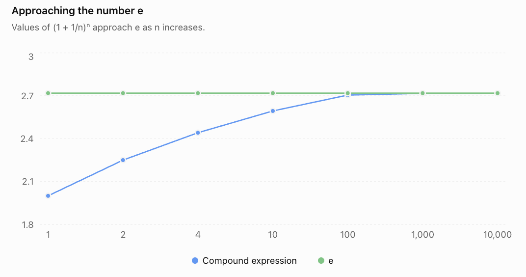
This limit helps explain why e appears in continuously compounded interest.
Natural Exponential Functions
A natural exponential function has the form:
f(x) = eˣ
More generally:
f(x) = Aeᵏˣ
Where:
-
A = initial value or scaling constant.
-
k = exponential growth or decay constant.
-
x = independent variable.
When k > 0, the function represents exponential growth.
When k < 0, it represents exponential decay.
Graph of y = eˣ
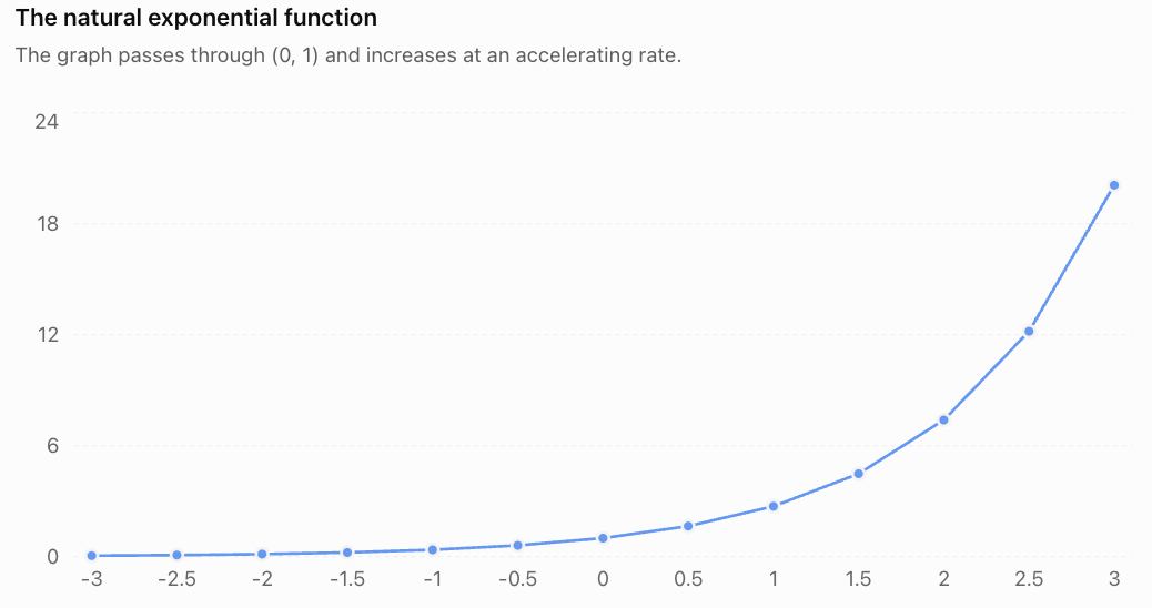
Important properties include:
-
Domain: all real numbers.
-
Range: y > 0.
-
y-intercept: (0, 1).
-
Horizontal asymptote: y = 0.
-
The function is continuous and differentiable everywhere.
-
The function is always increasing.
-
Its derivative is equal to the function itself.
The final property makes eˣ especially important in calculus.
Understanding Rates of Change
Calculus is fundamentally concerned with change.
A rate of change describes how quickly one quantity changes in relation to another.
For a function y = f(x), the average rate of change between x = a and x = b is:
Average rate of change = [f(b) − f(a)]/(b − a)
This is the slope of the secant line connecting two points on the graph.
Worked Example 1: Average Rate of Exponential Change
Consider:
f(x) = eˣ
Calculate the average rate of change between x = 0 and x = 2.
Step 1: Evaluate the function.
f(0) = e⁰ = 1
f(2) = e² ≈ 7.3891
Step 2: Apply the formula.
Average rate = (7.3891 − 1)/(2 − 0)
Average rate = 6.3891/2
Average rate ≈ 3.1945
The function increases by an average of approximately 3.1945 units of y per unit of x over this interval.
However, the function does not increase at a constant rate.
Its instantaneous rate of change increases as x increases.
Instantaneous Rate of Change
The instantaneous rate of change measures how quickly a function changes at a particular point.
Geometrically, it is the slope of the tangent line at that point.
This is the central idea behind differentiation.
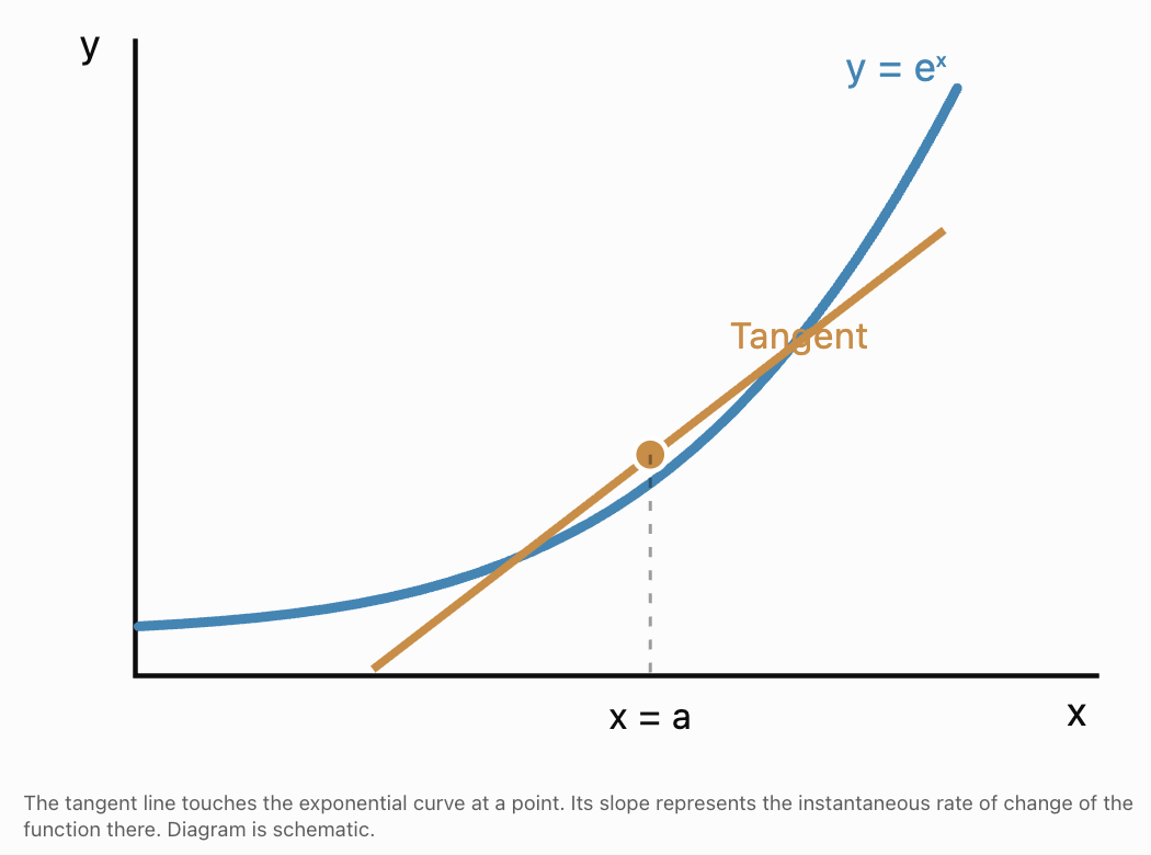
The derivative
The derivative of a function f(x) is written:
f′(x)
or:
dy/dx
The derivative measures the instantaneous rate of change.
It is defined using a limit:
f′(x) = lim(h → 0) [f(x + h) − f(x)]/h
This is called the limit definition of the derivative.
The derivative describes what happens to the average rate of change as the interval becomes arbitrarily small.
Why e Is Special in Differentiation
Consider the exponential function:
f(x) = eˣ
Using the limit definition:
f′(x) = lim(h → 0) [e^(x+h) − eˣ]/h
Use the exponent rule:
e^(x+h) = eˣeʰ
Therefore:
f′(x) = lim(h → 0) [eˣeʰ − eˣ]/h
Factor out eˣ:
f′(x) = eˣ lim(h → 0) [(eʰ − 1)/h]
A fundamental limit is:
lim(h → 0) [(eʰ − 1)/h] = 1
Therefore:
d/dx(eˣ) = eˣ
This is one of the most important results in calculus.
The derivative of eˣ is exactly eˣ.
Interpreting the result
At x = 0:
e⁰ = 1
The slope of the tangent line is also 1.
At x = 1:
e¹ ≈ 2.718
The slope is approximately 2.718.
At x = 2:
e² ≈ 7.389
The slope is approximately 7.389.
|
x |
eˣ |
Slope of tangent |
|---|---|---|
|
−2 |
0.1353 |
0.1353 |
|
−1 |
0.3679 |
0.3679 |
|
0 |
1.0000 |
1.0000 |
|
1 |
2.7183 |
2.7183 |
|
2 |
7.3891 |
7.3891 |
As the function increases, its instantaneous rate of increase also increases.
Differentiating General Exponential Functions
For the natural exponential function:
d/dx(eᵏˣ) = keᵏˣ
This follows from the chain rule.
More generally:
d/dx(Aeᵏˣ) = Akeᵏˣ
Where A and k are constants.
Worked Example 2: Differentiating an Exponential Function
Find the derivative of:
f(x) = 5e³ˣ
Use:
d/dx(Aeᵏˣ) = Akeᵏˣ
Substitute:
f′(x) = 5 × 3e³ˣ
f′(x) = 15e³ˣ
Worked Example 3: Exponential Decay
Find the derivative of:
f(t) = 200e⁻⁰·⁴ᵗ
Using the same rule:
f′(t) = 200(−0.4)e⁻⁰·⁴ᵗ
f′(t) = −80e⁻⁰·⁴ᵗ
The derivative is negative, indicating that the quantity decreases over time.
Its magnitude becomes smaller as the quantity approaches zero.
Differentiating Exponential Functions with Other Bases
Not every exponential function uses base e.
Consider:
f(x) = aˣ
where a > 0 and a ≠ 1.
The derivative is:
d/dx(aˣ) = aˣln(a)
For example:
d/dx(2ˣ) = 2ˣln(2)
d/dx(5ˣ) = 5ˣln(5)
d/dx(10ˣ) = 10ˣln(10)
Why does the natural exponential function have such a simple derivative?
Because:
ln(e) = 1
Therefore:
d/dx(eˣ) = eˣln(e) = eˣ
Worked Example 4: Differentiating 2ˣ
Find the derivative of:
f(x) = 2ˣ
Use:
f′(x) = 2ˣln(2)
Since ln(2) ≈ 0.693147:
f′(x) ≈ 0.693147 × 2ˣ
At x = 3:
f′(3) = 2³ln(2)
f′(3) = 8(0.693147)
f′(3) ≈ 5.5452
The instantaneous rate of change at x = 3 is approximately 5.5452.
Interpreting Rates in Exponential Models
Suppose a population follows:
P(t) = P₀eʳᵗ
Differentiate:
P′(t) = rP₀eʳᵗ
Since P(t) = P₀eʳᵗ:
P′(t) = rP(t)
This tells us that the instantaneous population growth rate is proportional to the current population.
Worked Example 5: Population Growth Rate
A bacterial population is modelled by:
P(t) = 500e⁰·²ᵗ
where t is measured in hours.
Calculate the population and its instantaneous growth rate after five hours.
Step 1: Calculate the population.
P(5) = 500e¹
P(5) ≈ 500(2.71828)
P(5) ≈ 1,359 bacteria
Step 2: Differentiate.
P′(t) = 500(0.2)e⁰·²ᵗ
P′(t) = 100e⁰·²ᵗ
Step 3: Evaluate at t = 5.
P′(5) = 100e¹
P′(5) ≈ 272 bacteria per hour
Interpretation
After five hours, the model predicts approximately 1,359 bacteria.
At that instant, the population is increasing at approximately 272 bacteria per hour.
The population and growth rate are different quantities.
The population is measured in bacteria.
The instantaneous growth rate is measured in bacteria per hour.
Exponential Decay and Derivatives
For exponential decay:
N(t) = N₀e⁻λᵗ
where λ > 0.
Differentiate:
N′(t) = −λN₀e⁻λᵗ
Therefore:
N′(t) = −λN(t)
The negative sign indicates that the quantity is decreasing.
The magnitude of the rate of decay is:
|N′(t)| = λN(t)
This means that a larger radioactive sample has a greater expected number of decays per unit time.
Worked Example 6: Radioactive Decay Rate
A radioactive sample follows:
N(t) = 10000e⁻⁰·¹ᵗ
where t is measured in years.
Calculate the expected number of undecayed nuclei and the instantaneous decay rate after 10 years.
Step 1: Calculate the quantity remaining.
N(10) = 10000e⁻¹
N(10) ≈ 10000(0.367879)
N(10) ≈ 3,679 nuclei
Step 2: Differentiate.
N′(t) = −1000e⁻⁰·¹ᵗ
Step 3: Evaluate.
N′(10) = −1000e⁻¹
N′(10) ≈ −367.88 nuclei per year
The negative value indicates a decreasing population of undecayed nuclei.
The expected rate of decay at that time is approximately 368 nuclei per year.
Connecting Exponential Functions to Integration
Differentiation measures instantaneous rates of change.
Integration is closely related to accumulation and total change.
An integral can be used to calculate quantities such as:
-
Total population increase over a time interval.
-
Accumulated radioactive decays.
-
Total energy transferred.
-
Total fluid flowing through a system.
-
Accumulated interest under suitable models.
The indefinite integral
An indefinite integral represents a family of antiderivatives.
Because:
d/dx(eˣ) = eˣ
we have:
∫eˣ dx = eˣ + C
Where C is the constant of integration.
Why do we need C?
The derivative of eˣ is eˣ.
But the derivative of eˣ + 5 is also eˣ.
Likewise, the derivative of eˣ − 12 is eˣ.
Every constant disappears during differentiation.
Therefore, indefinite integration includes an arbitrary constant.
Integrating General Exponential Functions
For k ≠ 0:
∫eᵏˣ dx = (1/k)eᵏˣ + C
More generally:
∫Aeᵏˣ dx = (A/k)eᵏˣ + C
Worked Example 7: Integrating an Exponential Function
Evaluate:
∫6e²ˣ dx
Use:
∫Aeᵏˣ dx = (A/k)eᵏˣ + C
Therefore:
∫6e²ˣ dx = (6/2)e²ˣ + C
Answer: 3e²ˣ + C
Checking the answer
Differentiate:
d/dx(3e²ˣ) = 3(2)e²ˣ
= 6e²ˣ
This matches the original integrand.
Definite Integrals and Accumulation
A definite integral calculates accumulated change over an interval.
For example:
∫ₐᵇ eˣ dx = eᵇ − eᵃ
This follows from the Fundamental Theorem of Calculus.
Worked Example 8: Evaluating a Definite Integral
Evaluate:
∫₀² eˣ dx
Step 1: Find an antiderivative.
∫eˣ dx = eˣ + C
Step 2: Apply the limits.
∫₀² eˣ dx = e² − e⁰
= e² − 1
Step 3: Evaluate.
≈ 7.389056 − 1
Answer ≈ 6.3891
Visualising the area
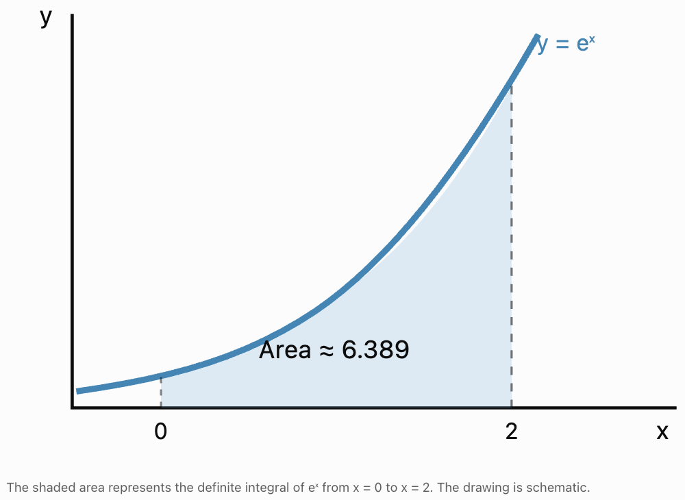
The definite integral represents the area under the curve between the two limits because eˣ is positive.
The Fundamental Theorem of Calculus
The Fundamental Theorem of Calculus connects differentiation and integration.
In simplified terms:
Differentiation and integration are inverse processes, up to an additive constant.
If F′(x) = f(x), then:
∫ₐᵇ f(x) dx = F(b) − F(a)
For exponential functions:
If f(x) = eˣ, then F(x) = eˣ.
Therefore:
∫ₐᵇ eˣ dx = eᵇ − eᵃ
This connection allows us to move between instantaneous rates and accumulated quantities.
Example: Population Change
Suppose:
P′(t) = 100e⁰·²ᵗ
The total population increase from t = 0 to t = 5 is:
∫₀⁵ 100e⁰·²ᵗ dt
Integrate:
= [500e⁰·²ᵗ]₀⁵
= 500e¹ − 500e⁰
= 500(e − 1)
≈ 500(1.71828)
Total population increase ≈ 859 organisms
This matches the difference between the population at t = 5 and the initial population.
Differential Equations and Exponential Functions
A differential equation is an equation involving a function and one or more of its derivatives.
Exponential functions are particularly important because they naturally solve many differential equations.
Consider:
dy/dt = ky
This equation states:
"The instantaneous rate of change of y is proportional to y itself."
Its general solution is:
y(t) = Ceᵏᵗ
where C is a constant determined by an initial condition.
Why does this work?
Suppose:
y(t) = Ceᵏᵗ
Differentiate:
dy/dt = Ckeᵏᵗ
Factor out k:
dy/dt = k(Ceᵏᵗ)
Since y = Ceᵏᵗ:
dy/dt = ky
Therefore, the exponential function satisfies the differential equation.
Worked Example 9: Solving a Differential Equation
A population satisfies:
dP/dt = 0.3P
Initially:
P(0) = 400
Find P(t).
Step 1: Identify the general solution.
P(t) = Ce⁰·³ᵗ
Step 2: Apply the initial condition.
P(0) = Ce⁰
400 = C
Step 3: Write the particular solution.
P(t) = 400e⁰·³ᵗ
Calculate the population after four years
P(4) = 400e¹·²
Since e¹·² ≈ 3.320117:
P(4) ≈ 400 × 3.320117
P(4) ≈ 1,328 organisms
The differential equation describes the rate of growth.
The exponential solution describes the population itself.
Connections to Advanced Mathematics
Exponential functions appear throughout higher mathematics.
1. Differential Equations
Exponential functions solve equations in which rates of change depend on current values.
Applications include population growth, radioactive decay, electrical circuits, and chemical kinetics.
2. Calculus of Several Variables
Exponential functions can depend on more than one variable.
For example:
f(x, t) = Ae⁻ᵏᵗ sin(x)
Such functions appear in mathematical models involving time-dependent waves, diffusion, and other physical processes.
Partial derivatives describe how the function changes with respect to one variable while holding others constant.
3. Complex Numbers
Exponential functions extend naturally to complex numbers.
One of the most famous mathematical identities is Euler's formula:
eⁱᶿ = cos(θ) + i sin(θ)
where i² = −1.
This connects exponential functions, trigonometry, and complex numbers.
For θ = π:
eⁱπ = −1
Therefore:
eⁱπ + 1 = 0
This is known as Euler's identity.
4. Probability and Statistics
The exponential function appears in probability distributions.
For example, the exponential distribution has probability density function:
f(t) = λe⁻λᵗ, for t ≥ 0
where λ > 0.
It can model waiting times between events in certain random processes with constant event rates.
5. Advanced Mathematical Modelling
Exponential functions also appear in:
-
Heat transfer.
-
Electrical circuit analysis.
-
Pharmacokinetics.
-
Chemical reaction rates.
-
Population dynamics.
-
Financial mathematics.
-
Signal processing.
-
Machine learning.
The importance of exponential functions comes from their ability to connect mathematical structure with changing real-world systems.
Authentic Application: A Cooling System
An electronic component begins at 90°C in a room maintained at 25°C.
Its temperature follows:
T(t) = 25 + 65e⁻⁰·¹ᵗ
where t is measured in minutes.
We want to calculate its temperature, cooling rate, and the time required to reach 40°C.
Part A: Calculate the temperature after 10 minutes
T(10) = 25 + 65e⁻¹
Since e⁻¹ ≈ 0.367879:
T(10) ≈ 25 + 65(0.367879)
T(10) ≈ 25 + 23.9121
T(10) ≈ 48.91°C
Part B: Find the instantaneous cooling rate
Differentiate:
T′(t) = 65(−0.1)e⁻⁰·¹ᵗ
T′(t) = −6.5e⁻⁰·¹ᵗ
At t = 10:
T′(10) = −6.5e⁻¹
T′(10) ≈ −6.5(0.367879)
T′(10) ≈ −2.39°C/min
The component is cooling at approximately 2.39°C per minute after 10 minutes.
Part C: Find when the temperature reaches 40°C
Set:
40 = 25 + 65e⁻⁰·¹ᵗ
Subtract 25:
15 = 65e⁻⁰·¹ᵗ
Divide by 65:
15/65 = e⁻⁰·¹ᵗ
Take natural logarithms:
ln(15/65) = −0.1t
Therefore:
t = ln(15/65)/(−0.1)
t ≈ 14.66 minutes
The model predicts that the component reaches 40°C after approximately 14.66 minutes.
Part D: Interpret the model
The temperature approaches the ambient temperature of 25°C.
The cooling rate is initially relatively large because the temperature difference is large.
As the component cools, the temperature difference decreases, so the magnitude of the cooling rate becomes smaller.
This is a practical example of how exponential functions, differentiation, logarithms, and differential equations work together.
Common Mistakes
Mistake 1: Confusing e with a variable
The symbol e represents a mathematical constant.
Correction: Remember that e ≈ 2.71828.
Mistake 2: Assuming all exponential derivatives are unchanged
The derivative of eˣ is eˣ, but the derivative of e³ˣ is 3e³ˣ.
Correction: Apply the chain rule.
Mistake 3: Forgetting the logarithm when differentiating aˣ
The derivative of aˣ is aˣln(a).
Correction: Remember that the natural exponential function is the special case where a = e.
Mistake 4: Confusing a function with its derivative
The population and its rate of growth are different quantities.
Correction: Check the units of each result.
Mistake 5: Forgetting the negative sign in exponential decay
For e⁻λᵗ, the derivative includes a factor of −λ.
Correction: Differentiate the exponent carefully.
Mistake 6: Forgetting the constant of integration
Indefinite integrals require + C.
Correction: Include the arbitrary constant unless evaluating a definite integral.
Mistake 7: Multiplying instead of dividing during integration
The integral of e³ˣ is (1/3)e³ˣ + C, not 3e³ˣ + C.
Correction: Reverse the chain rule.
Mistake 8: Confusing average and instantaneous rates
Average rate of change is calculated over an interval.
Instantaneous rate of change is calculated at a particular point.
Correction: Use secant slopes for averages and derivatives for instantaneous rates.
Mistake 9: Ignoring units
A derivative represents a rate, so its units differ from those of the original quantity.
Correction: State units clearly.
Mistake 10: Treating a mathematical model as exact reality
Exponential models depend on assumptions.
Correction: Evaluate whether the underlying process is appropriately represented.
Key Terms
-
Calculus: Branch of mathematics concerned with change and accumulation.
-
e: Irrational mathematical constant approximately equal to 2.71828.
-
Natural Exponential Function: Exponential function with base e.
-
Limit: Value approached by a function or sequence.
-
Rate of Change: Measure of how one quantity changes relative to another.
-
Average Rate of Change: Change in a function divided by change in its independent variable over an interval.
-
Instantaneous Rate of Change: Rate of change at a particular point.
-
Derivative: Mathematical expression describing instantaneous rate of change.
-
Differentiation: Process of finding derivatives.
-
Tangent Line: Line whose slope represents the instantaneous rate of change at a point on a differentiable curve.
-
Secant Line: Line passing through two points on a curve.
-
Chain Rule: Rule for differentiating composite functions.
-
Integral: Mathematical expression related to accumulation and antiderivatives.
-
Indefinite Integral: Family of antiderivatives.
-
Definite Integral: Integral evaluated over a specified interval.
-
Antiderivative: Function whose derivative is a given function.
-
Constant of Integration: Arbitrary constant added to an indefinite integral.
-
Fundamental Theorem of Calculus: Theorem connecting differentiation and integration.
-
Differential Equation: Equation involving a function and its derivatives.
-
Initial Condition: Specified value used to determine a particular solution.
-
Exponential Growth Constant: Parameter describing proportional exponential growth.
-
Decay Constant: Positive parameter describing exponential decay.
-
Euler's Formula: Identity connecting complex exponentials with trigonometric functions.
-
Euler's Identity: Special case eⁱπ + 1 = 0.
-
Mathematical Model: Mathematical representation of a real-world process.
Key Takeaways
-
The number e arises naturally in continuous growth and compounding.
-
The natural exponential function eˣ has the special property that its derivative equals itself.
-
Derivatives measure instantaneous rates of change.
-
Exponential growth models have rates proportional to their current values.
-
Exponential decay models have negative derivatives.
-
The derivative of Aeᵏˣ is Akeᵏˣ.
-
The derivative of aˣ is aˣln(a).
-
Integration reverses differentiation, up to an additive constant.
-
The integral of eᵏˣ is (1/k)eᵏˣ + C for k ≠ 0.
-
Definite integrals can calculate accumulated change.
-
Exponential functions solve differential equations of the form dy/dt = ky.
-
Exponential functions connect calculus with complex numbers, probability, physics, biology, and engineering.
-
Understanding exponential functions provides a foundation for advanced mathematical modelling.
Check Your Understanding
Questions
Question 1: The Number e
Explain why e appears naturally in continuously compounded interest.
Question 2: Natural Exponential Functions
State the value of e⁰ and explain its importance for the graph of y = eˣ.
Question 3: Average Rate of Change
Calculate the average rate of change of f(x) = eˣ between x = 0 and x = 1.
Question 4: Differentiation
Differentiate:
f(x) = eˣ
Question 5: Chain Rule
Differentiate:
f(x) = 4e²ˣ
Question 6: Exponential Decay
Differentiate:
N(t) = 500e⁻⁰·³ᵗ
Question 7: Other Exponential Bases
Differentiate:
f(x) = 3ˣ
Question 8: Population Growth Rate
A population follows:
P(t) = 200e⁰·⁴ᵗ
Calculate the instantaneous growth rate at t = 3.
Question 9: Indefinite Integration
Evaluate:
∫5eˣ dx
Question 10: Integration with the Chain Rule
Evaluate:
∫8e⁴ˣ dx
Question 11: Definite Integration
Evaluate:
∫₀¹ e²ˣ dx
Question 12: Differential Equations
Solve:
dy/dt = 0.2y
given:
y(0) = 300
Question 13: Cooling Model
An object follows:
T(t) = 20 + 50e⁻⁰·²ᵗ
Calculate its instantaneous cooling rate at t = 5.
Question 14: Conceptual Understanding
Explain why the derivative of eˣ is especially important in calculus.
Question 15: Connecting Calculus and Modelling
A population grows according to:
P(t) = 1000e⁰·¹ᵗ
Calculate:
a) The population after 10 years.
b) The instantaneous growth rate after 10 years.
c) The total population increase over the first 10 years.
Fully Worked Answers
Answer 1: The Number e
The number e appears when interest is compounded increasingly frequently.
The expression:
(1 + 1/n)ⁿ
approaches e as n approaches infinity.
This leads to the continuous compounding formula:
A = Peʳᵗ
Answer 2: Natural Exponential Functions
e⁰ = 1
Therefore:
f(0) = 1
The graph of y = eˣ passes through:
(0, 1)
Answer 3: Average Rate of Change
Average rate:
[f(1) − f(0)]/(1 − 0)
= (e − 1)/1
= e − 1
Average rate ≈ 1.7183
Answer 4: Differentiation
Given:
f(x) = eˣ
The derivative is:
f′(x) = eˣ
Answer 5: Chain Rule
Given:
f(x) = 4e²ˣ
Differentiate:
f′(x) = 4(2)e²ˣ
f′(x) = 8e²ˣ
Answer 6: Exponential Decay
Given:
N(t) = 500e⁻⁰·³ᵗ
Differentiate:
N′(t) = 500(−0.3)e⁻⁰·³ᵗ
N′(t) = −150e⁻⁰·³ᵗ
Answer 7: Other Exponential Bases
Given:
f(x) = 3ˣ
Use:
d/dx(aˣ) = aˣln(a)
Therefore:
f′(x) = 3ˣln(3)
Answer 8: Population Growth Rate
Given:
P(t) = 200e⁰·⁴ᵗ
Differentiate:
P′(t) = 80e⁰·⁴ᵗ
At t = 3:
P′(3) = 80e¹·²
Since e¹·² ≈ 3.320117:
P′(3) ≈ 80(3.320117)
P′(3) ≈ 265.61 organisms per time unit
Answer 9: Indefinite Integration
Evaluate:
∫5eˣ dx
Since the antiderivative of eˣ is eˣ:
Answer: 5eˣ + C
Answer 10: Integration with the Chain Rule
Evaluate:
∫8e⁴ˣ dx
Use:
∫Aeᵏˣ dx = (A/k)eᵏˣ + C
Therefore:
∫8e⁴ˣ dx = (8/4)e⁴ˣ + C
Answer: 2e⁴ˣ + C
Answer 11: Definite Integration
Evaluate:
∫₀¹ e²ˣ dx
Antiderivative:
(1/2)e²ˣ
Apply the limits:
= (1/2)e² − (1/2)e⁰
= (e² − 1)/2
Since e² ≈ 7.389056:
= (7.389056 − 1)/2
Answer ≈ 3.1945
Answer 12: Differential Equations
Given:
dy/dt = 0.2y
General solution:
y(t) = Ce⁰·²ᵗ
Apply the initial condition:
y(0) = 300
300 = Ce⁰
C = 300
Answer: y(t) = 300e⁰·²ᵗ
Answer 13: Cooling Model
Given:
T(t) = 20 + 50e⁻⁰·²ᵗ
Differentiate:
T′(t) = −10e⁻⁰·²ᵗ
At t = 5:
T′(5) = −10e⁻¹
T′(5) ≈ −10(0.367879)
T′(5) ≈ −3.68°C per time unit
The negative sign indicates that the object is cooling.
Answer 14: Conceptual Understanding
The derivative of eˣ is equal to eˣ.
This means that the instantaneous rate of change of the function is equal to its current value.
This property makes exponential functions natural solutions to differential equations involving proportional growth and decay.
It also simplifies differentiation, integration, and advanced mathematical modelling.
Answer 15: Connecting Calculus and Modelling
Given:
P(t) = 1000e⁰·¹ᵗ
Part a: Population after 10 years
P(10) = 1000e¹
P(10) ≈ 1000(2.71828)
P(10) ≈ 2,718 organisms
Part b: Instantaneous growth rate
Differentiate:
P′(t) = 100e⁰·¹ᵗ
At t = 10:
P′(10) = 100e¹
P′(10) ≈ 271.83 organisms per year
Part c: Total population increase
Initial population:
P(0) = 1000
Population after 10 years:
P(10) ≈ 2718.28
Total increase:
2718.28 − 1000
Total increase ≈ 1,718 organisms
We can also calculate this using integration:
∫₀¹⁰ P′(t) dt = ∫₀¹⁰ 100e⁰·¹ᵗ dt
= [1000e⁰·¹ᵗ]₀¹⁰
= 1000e − 1000
≈ 1718.28
Both methods produce the same result.
Final Reflection
Exponential functions provide one of the most important connections between algebra and calculus.
The number e is especially significant because the natural exponential function has the remarkable property that its derivative is equal to itself.
This allows exponential functions to describe processes in which the instantaneous rate of change is proportional to the current quantity.
Differentiation helps us calculate rates of growth and decay, while integration allows us to calculate accumulated changes. Differential equations bring these ideas together to describe how real systems evolve.
These relationships extend far beyond introductory calculus into physics, chemistry, biology, engineering, finance, probability, and advanced mathematics.
Understanding exponential functions is therefore more than learning a particular family of equations. It is developing a mathematical language for describing change, accumulation, and the relationships between quantities and their rates of change.
5. Comprehensive Problem Solving
Learning outcomes
- I can solve complex multi-step exponential and logarithmic problems.
- I can integrate concepts from throughout the course.
- I can select efficient mathematical strategies.
- I can justify mathematical reasoning.
- I can communicate complete mathematical solutions.
Introduction
Exponential and logarithmic functions are powerful mathematical tools for understanding situations involving growth, decay, multiplication, changing rates, and quantities that span enormous numerical ranges.
Throughout this course, we have studied exponential functions, logarithms, equations, inequalities, transformations, mathematical models, financial applications, scientific applications, technological growth, and connections to calculus.
The purpose of comprehensive problem solving is to combine these ideas to solve unfamiliar, multi-step problems.
A complex problem rarely tells us which formula to use. Instead, we must interpret the information, identify mathematical relationships, select an efficient strategy, perform calculations accurately, and explain what our answers mean.
For example:
-
How can we compare two investments with different compounding methods?
-
When will a growing population reach a particular size?
-
How can we estimate the age of a radioactive sample?
-
How can we determine whether a dataset is exponential?
-
How can we solve equations containing several exponential or logarithmic expressions?
-
How can derivatives and logarithms help us analyse a changing system?
These problems require more than memorising formulas. They require mathematical reasoning, careful organisation, and the ability to connect different concepts.
A Framework for Complex Mathematical Problems
A reliable problem-solving process can be organised into six stages.
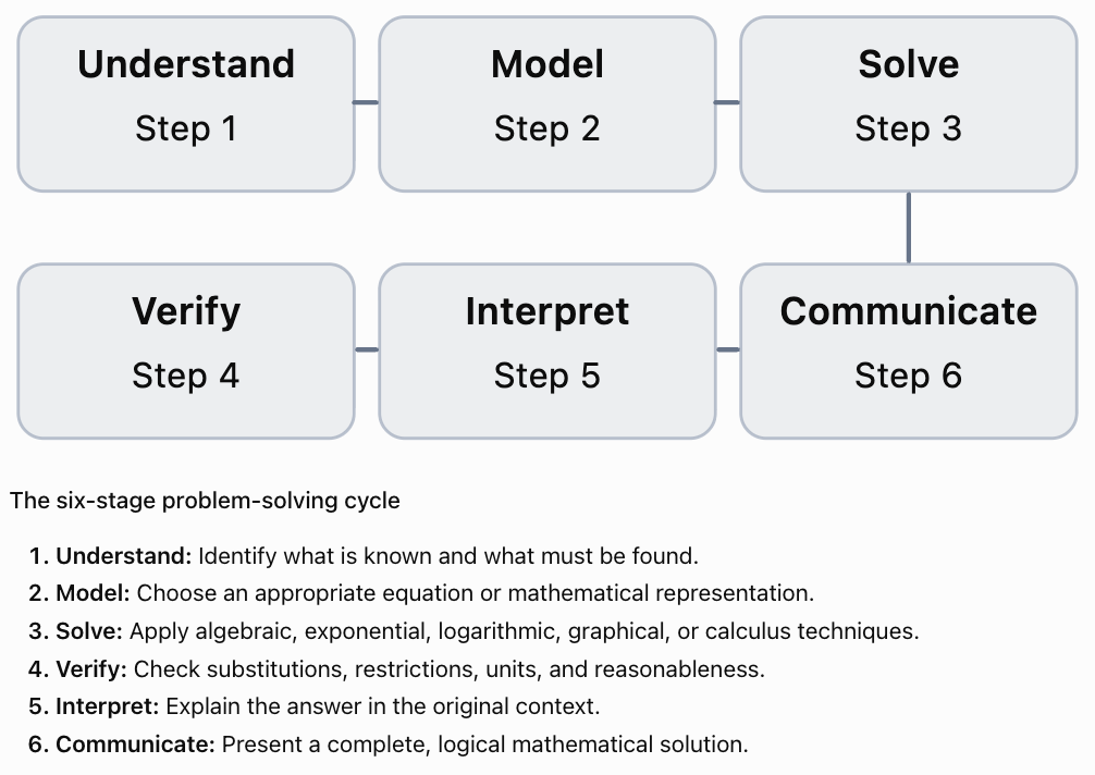
A strong solution should demonstrate all six stages, even when some are completed mentally.
Essential Mathematical Relationships
The following formulas connect many of the topics studied throughout the course.
|
Concept |
Key relationship |
|---|---|
|
y = abˣ |
|
|
Natural exponential function |
y = Aeᵏˣ |
|
Logarithmic definition |
logₐ(x) = y ⇔ aʸ = x |
|
Product law |
logₐ(MN) = logₐ(M) + logₐ(N) |
|
Quotient law |
logₐ(M/N) = logₐ(M) − logₐ(N) |
|
Power law |
logₐ(Mᵖ) = p logₐ(M) |
|
Change of base |
logₐ(x) = ln(x)/ln(a) |
|
Exponential growth |
P(t) = P₀eʳᵗ |
|
Exponential decay |
N(t) = N₀e⁻λᵗ |
|
Half-life |
t½ = ln(2)/λ |
|
Doubling time |
tᵈ = ln(2)/r |
|
Compound interest |
A = P(1 + r/m)^(mt) |
|
Continuous compounding |
A = Peʳᵗ |
|
Logistic growth |
P(t) = K/(1 + Ae⁻ʳᵗ) |
|
Exponential derivative |
d/dx(eᵏˣ) = keᵏˣ |
|
Exponential integral |
∫eᵏˣ dx = eᵏˣ/k + C, k ≠ 0 |
For logarithmic laws, the arguments M and N must be positive, and the base a must be positive and not equal to 1.
Selecting an Efficient Mathematical Strategy
The structure of a problem often suggests the most efficient approach.
|
Problem type |
Recommended strategy |
|---|---|
|
Same exponential base on both sides |
Rewrite using common bases |
|
Different exponential bases |
Take logarithms |
|
Several powers of the same exponential |
Substitute u = aˣ |
|
Logarithmic expressions |
Combine logarithms and check domains |
|
Unknown growth or decay time |
Isolate the exponential and use logarithms |
|
Growth constant from measurements |
Use ratios and natural logarithms |
|
Comparing models |
Solve for intersections or compare predictions |
|
Exponential inequality |
Consider whether the base is above or below 1 |
|
Rate of change |
Differentiate |
|
Accumulated change |
Integrate |
|
Real-world model |
Check assumptions, units, and context |
Choosing a strategy before calculating can prevent unnecessary algebra and reduce errors.
Solving Advanced Exponential Equations
Worked Example 1: Equations with a Common Base
Solve:
3^(2x − 1) = 81^(x − 2)
Step 1: Express both sides using base 3.
Since 81 = 3⁴:
3^(2x − 1) = 3^[4(x − 2)]
Step 2: Equate the exponents.
2x − 1 = 4x − 8
Step 3: Solve.
7 = 2x
x = 3.5
Step 4: Verify.
Left side:
3^(2 × 3.5 − 1) = 3⁶ = 729
Right side:
81^(3.5 − 2) = 81¹·⁵ = 729
Both sides agree.
Worked Example 2: Exponential Equations Requiring Substitution
Solve:
4ˣ − 5(2ˣ) + 4 = 0
Notice that:
4ˣ = (2ˣ)²
Step 1: Substitute.
Let:
u = 2ˣ
Then:
u² − 5u + 4 = 0
Step 2: Factorise.
(u − 1)(u − 4) = 0
Therefore:
u = 1 or u = 4
Step 3: Substitute back.
If 2ˣ = 1:
x = 0
If 2ˣ = 4:
x = 2
Solutions: x = 0 or x = 2
This substitution transforms an exponential equation into a familiar quadratic equation.
Worked Example 3: Different Exponential Bases
Solve:
5^(x + 1) = 3^(2x)
Step 1: Take natural logarithms.
ln[5^(x + 1)] = ln[3^(2x)]
Step 2: Apply the power law.
(x + 1)ln(5) = 2x ln(3)
Step 3: Expand.
x ln(5) + ln(5) = 2x ln(3)
Step 4: Collect terms.
ln(5) = x[2ln(3) − ln(5)]
Step 5: Solve.
x = ln(5)/[2ln(3) − ln(5)]
Using:
ln(5) ≈ 1.609438
ln(3) ≈ 1.098612
x ≈ 1.609438/(2.197225 − 1.609438)
x ≈ 2.738
The logarithmic method is efficient because the two exponential expressions cannot easily be rewritten using a common base.
Solving Advanced Logarithmic Equations
Logarithmic equations require particular care because the arguments of logarithms must be positive.
Worked Example 4: Combining Logarithms
Solve:
log₂(x − 1) + log₂(x − 3) = 3
Step 1: Identify domain restrictions.
x − 1 > 0
x − 3 > 0
Therefore:
x > 3
Step 2: Apply the product law.
log₂[(x − 1)(x − 3)] = 3
Step 3: Convert to exponential form.
(x − 1)(x − 3) = 2³
(x − 1)(x − 3) = 8
Step 4: Expand.
x² − 4x + 3 = 8
x² − 4x − 5 = 0
Step 5: Factorise.
(x − 5)(x + 1) = 0
Therefore:
x = 5 or x = −1
Step 6: Check the domain.
Only x = 5 satisfies x > 3.
Final answer: x = 5
The solution x = −1 is extraneous because it makes the logarithmic arguments invalid.
Worked Example 5: Logarithms with Different Bases
Solve:
log₂(x) + log₄(x) = 6
Step 1: Express the logarithms using a common base.
Since 4 = 2²:
log₄(x) = log₂(x)/2
Step 2: Substitute.
log₂(x) + (1/2)log₂(x) = 6
Step 3: Combine like terms.
(3/2)log₂(x) = 6
log₂(x) = 4
Step 4: Convert to exponential form.
x = 2⁴
x = 16
Check:
log₂(16) = 4
log₄(16) = 2
4 + 2 = 6
The solution is correct.
Exponential and Logarithmic Inequalities
Inequalities require attention to the direction of the inequality sign.
For an exponential function with base greater than 1, the function is increasing.
For a base between 0 and 1, the function is decreasing.
Worked Example 6: Exponential Inequality
Solve:
2^(3x − 1) > 16
Rewrite:
16 = 2⁴
Therefore:
2^(3x − 1) > 2⁴
Because base 2 is greater than 1:
3x − 1 > 4
3x > 5
x > 5/3
Worked Example 7: Decreasing Exponential Function
Solve:
(1/3)^(2x + 1) ≤ 1/27
Rewrite:
1/27 = (1/3)³
Therefore:
(1/3)^(2x + 1) ≤ (1/3)³
Since 0 < 1/3 < 1, the exponential function is decreasing.
The inequality reverses when comparing exponents:
2x + 1 ≥ 3
2x ≥ 2
x ≥ 1
Worked Example 8: Logarithmic Inequality
Solve:
ln(x − 2) ≥ 1
Step 1: Identify the domain.
x − 2 > 0
x > 2
Step 2: Convert to exponential form.
Because ln(x) is increasing:
x − 2 ≥ e¹
Step 3: Solve.
x ≥ 2 + e
Approximately:
x ≥ 4.718
This satisfies the original domain restriction.
Comparing Exponential Models
Some problems require us to compare two exponential functions and determine when one becomes greater than the other.
Worked Example 9: Comparing Two Technologies
Two hypothetical computing systems have processing capacities:
A(t) = 800(1.15)ᵗ
B(t) = 500(1.25)ᵗ
where t is measured in years.
Determine when System B overtakes System A.
Step 1: Set the models equal.
800(1.15)ᵗ = 500(1.25)ᵗ
Step 2: Divide by 500(1.15)ᵗ.
800/500 = (1.25/1.15)ᵗ
1.6 = (25/23)ᵗ
Step 3: Take logarithms.
ln(1.6) = t ln(25/23)
Step 4: Solve.
t = ln(1.6)/ln(25/23)
t ≈ 5.64 years
System B overtakes System A after approximately 5.64 years.
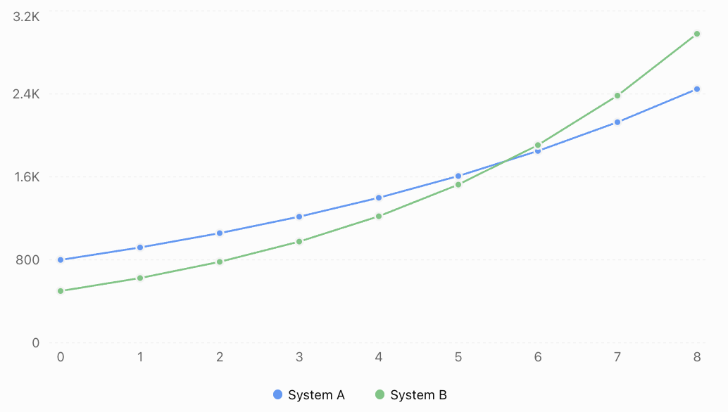
Interpretation
System A begins with greater capacity.
System B has a higher growth rate.
Although System B initially has a disadvantage, its faster exponential growth eventually allows it to overtake System A.
This is a common feature of competing exponential models.
Building Exponential Models from Data
Real-world problems often provide measurements rather than equations.
We must construct the mathematical model before solving the problem.
Worked Example 10: Determining an Exponential Model
A bacterial population is measured at two times.
|
Time (hours) |
Population |
|---|---|
|
0 |
400 |
|
6 |
1,200 |
Assume continuous exponential growth.
Find the growth model and predict the population after 10 hours.
Step 1: Choose the model.
P(t) = P₀eʳᵗ
Since P₀ = 400:
P(t) = 400eʳᵗ
Step 2: Use the second measurement.
1200 = 400e⁶ʳ
Divide by 400:
3 = e⁶ʳ
Step 3: Take natural logarithms.
ln(3) = 6r
r = ln(3)/6
r ≈ 0.1831 h⁻¹
Step 4: Write the model.
P(t) = 400e^[(ln(3)/6)t]
Equivalently:
P(t) = 400 × 3^(t/6)
Step 5: Predict the population after 10 hours.
P(10) = 400 × 3^(10/6)
P(10) ≈ 2,498 bacteria
Evaluating the model
The model assumes that the relative growth rate remains constant.
It may be appropriate over a short period when nutrients and space are plentiful.
Over longer periods, environmental limitations may reduce the growth rate.
A logistic model may eventually become more appropriate.
Multi-Step Financial Applications
Financial problems often combine exponential growth, logarithms, percentages, and comparison of alternative models.
Worked Example 11: Comparing Investment Strategies
An investor has $10,000 and is considering two accounts.
Account A: 5.5% annual interest compounded annually.
Account B: 5.4% nominal annual interest compounded monthly.
Determine which account produces the larger balance after 15 years.
Step 1: Calculate Account A.
A(t) = 10000(1.055)ᵗ
After 15 years:
A(15) = 10000(1.055)¹⁵
A(15) ≈ $22,324.77
Step 2: Calculate Account B.
B(t) = 10000(1 + 0.054/12)^(12t)
After 15 years:
B(15) = 10000(1.0045)¹⁸⁰
B(15) ≈ $22,440.85
Step 3: Compare.
Difference:
22440.85 − 22324.77
Difference ≈ $116.08
Account B produces approximately $116 more under the stated assumptions.
Justifying the result
Although Account B has a lower nominal annual interest rate, monthly compounding produces a higher effective annual rate.
Account A:
EAR = 5.5%
Account B:
EAR = (1.0045)¹² − 1
EAR ≈ 5.536%
Therefore, Account B produces slightly greater growth.
This comparison assumes constant rates and excludes fees, taxes, and other account conditions.
Multi-Step Scientific Applications
Worked Example 12: Radioactive Decay and Half-Life
A radioactive sample initially contains 600 g of a particular isotope.
After 12 years, 150 g of the isotope remains.
Assume exponential decay.
Determine:
a) The decay constant.
b) The half-life.
c) The amount remaining after 20 years.
d) The time required for the amount to fall below 50 g.
Part A: Find the decay constant
Use:
M(t) = M₀e⁻λᵗ
Substitute:
150 = 600e⁻¹²λ
Divide by 600:
0.25 = e⁻¹²λ
Take natural logarithms:
ln(0.25) = −12λ
Therefore:
λ = −ln(0.25)/12
λ ≈ 0.11552 year⁻¹
Part B: Find the half-life
t½ = ln(2)/λ
Substitute:
t½ = 0.693147/0.11552
t½ = 6 years
Part C: Calculate the amount after 20 years
Use the exact half-life form:
M(t) = 600(1/2)^(t/6)
At t = 20:
M(20) = 600(1/2)^(20/6)
M(20) ≈ 59.53 g
Part D: Find when the amount falls below 50 g
Set:
600(1/2)^(t/6) < 50
Divide by 600:
(1/2)^(t/6) < 1/12
Take natural logarithms:
(t/6)ln(1/2) < ln(1/12)
Since ln(1/2) is negative, the inequality reverses when dividing:
t/6 > ln(1/12)/ln(1/2)
Therefore:
t > 6ln(12)/ln(2)
t > 21.51 years
The expected remaining mass falls below 50 g after approximately 21.51 years.
Multi-Step Logarithmic Applications
Worked Example 13: Comparing Chemical Concentrations
Two dilute aqueous solutions have hydrogen ion concentrations:
Solution A: 2.5 × 10⁻³ mol/L
Solution B: 4.0 × 10⁻⁶ mol/L
Calculate:
a) The approximate pH of each solution.
b) The difference in pH.
c) The ratio of their hydrogen ion concentrations.
For sufficiently dilute solutions, use:
pH ≈ −log₁₀([H⁺])
Part A: Calculate the pH values
Solution A:
pH ≈ −log₁₀(2.5 × 10⁻³)
pH ≈ 2.602
Solution B:
pH ≈ −log₁₀(4.0 × 10⁻⁶)
pH ≈ 5.398
Part B: Calculate the pH difference
Difference:
5.398 − 2.602
Difference ≈ 2.796 pH units
Part C: Calculate the concentration ratio
Ratio:
(2.5 × 10⁻³)/(4.0 × 10⁻⁶)
= 625
Solution A has 625 times the hydrogen ion concentration of Solution B.
This is consistent with the logarithmic pH difference because:
10²·⁷⁹⁶ ≈ 625
The calculation illustrates how logarithmic differences correspond to multiplicative ratios.
Combining Exponential Models with Calculus
Calculus allows us to investigate not only how much a quantity changes, but also how quickly it changes.
Worked Example 14: Population Growth and Instantaneous Rate
A population follows:
P(t) = 800e⁰·¹⁵ᵗ
where t is measured in years.
Determine:
a) The population after eight years.
b) The instantaneous growth rate after eight years.
c) The time required for the population to reach 4,000.
Part A: Calculate the population
P(8) = 800e¹·²
Since e¹·² ≈ 3.320117:
P(8) ≈ 800 × 3.320117
P(8) ≈ 2,656 organisms
Part B: Differentiate
P′(t) = 800(0.15)e⁰·¹⁵ᵗ
P′(t) = 120e⁰·¹⁵ᵗ
At t = 8:
P′(8) = 120e¹·²
P′(8) ≈ 398.41 organisms per year
Part C: Solve for time
Set:
4000 = 800e⁰·¹⁵ᵗ
Divide by 800:
5 = e⁰·¹⁵ᵗ
Take natural logarithms:
ln(5) = 0.15t
t = ln(5)/0.15
t ≈ 10.73 years
Interpretation
After eight years, the population is approximately 2,656.
At that instant, the population is increasing at approximately 398 organisms per year.
The population reaches 4,000 after approximately 10.73 years.
This problem combines exponential modelling, differentiation, logarithmic equations, and interpretation of rates.
Logistic Models and Advanced Problem Solving
Exponential growth may be inappropriate when a quantity approaches a limiting value.
A logistic model has the form:
P(t) = K/(1 + Ae⁻ʳᵗ)
where K represents carrying capacity.
Worked Example 15: Logistic Population Growth
A population follows:
P(t) = 10000/(1 + 19e⁻⁰·⁴ᵗ)
where t is measured in years.
Determine:
a) The initial population.
b) The carrying capacity.
c) The population after five years.
d) The time required to reach 8,000.
Part A: Initial population
At t = 0:
P(0) = 10000/(1 + 19)
P(0) = 10000/20
Initial population = 500
Part B: Carrying capacity
The carrying capacity is the limiting value:
K = 10,000
Part C: Population after five years
P(5) = 10000/(1 + 19e⁻²)
Since e⁻² ≈ 0.135335:
P(5) ≈ 10000/[1 + 19(0.135335)]
P(5) ≈ 10000/3.57137
P(5) ≈ 2,800 organisms
Part D: Time required to reach 8,000
Set:
8000 = 10000/(1 + 19e⁻⁰·⁴ᵗ)
Rearrange:
1 + 19e⁻⁰·⁴ᵗ = 10000/8000
1 + 19e⁻⁰·⁴ᵗ = 1.25
Subtract 1:
19e⁻⁰·⁴ᵗ = 0.25
Divide by 19:
e⁻⁰·⁴ᵗ = 1/76
Take natural logarithms:
−0.4t = ln(1/76)
Therefore:
t = ln(76)/0.4
t ≈ 10.83 years
The population reaches 8,000 after approximately 10.83 years.
Comparing exponential and logistic models
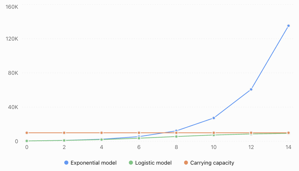
The exponential model continues increasing without bound.
The logistic model approaches a carrying capacity of 10,000.
Choosing between these models requires scientific understanding of the system.
Error Analysis and Verification
A mathematically correct calculation can still produce an inappropriate answer if the model is unsuitable or the assumptions are unrealistic.
Consider the following statement:
"A population doubles every year, so it will continue doubling forever."
The mathematical model might be:
P(t) = P₀2ᵗ
However, this model assumes an unlimited supply of resources and a constant proportional growth rate.
For a real biological population, these assumptions may fail.
Methods of verification
Algebraic verification
Substitute proposed solutions into the original equation.
Domain verification
Check that logarithmic arguments are positive.
Graphical verification
Compare calculated solutions with graphs.
Numerical verification
Use a calculator or spreadsheet to evaluate expressions.
Contextual verification
Check whether answers are physically, financially, or scientifically reasonable.
Dimensional verification
Check that units are consistent.
Worked Example 16: Identifying an Extraneous Solution
Solve:
ln(x − 2) + ln(x + 1) = ln(10)
Step 1: Identify the domain.
x − 2 > 0
x + 1 > 0
Therefore:
x > 2
Step 2: Combine logarithms.
ln[(x − 2)(x + 1)] = ln(10)
Step 3: Equate the arguments.
(x − 2)(x + 1) = 10
Expand:
x² − x − 2 = 10
x² − x − 12 = 0
Factorise:
(x − 4)(x + 3) = 0
Therefore:
x = 4 or x = −3
Step 4: Apply the domain restriction.
Only x = 4 satisfies x > 2.
Final answer: x = 4
The solution x = −3 must be rejected.
Communicating Mathematical Reasoning
A complete mathematical solution should be clear enough for another person to follow and verify.
Good mathematical communication includes:
-
Defining variables.
-
Stating relevant formulas.
-
Showing substitutions.
-
Explaining important algebraic steps.
-
Identifying domain restrictions.
-
Using appropriate units.
-
Rounding sensibly.
-
Interpreting results in context.
-
Justifying the selected model.
Example of weak communication
"Answer = 12.4."
This does not explain what was calculated or why the result is reasonable.
Example of strong communication
"Using the exponential decay model and the measured decay constant, the time required for the sample to decrease to the specified mass is approximately 12.4 years. The result is consistent with the decreasing exponential model because the target mass is smaller than the initial mass."
The second response connects the mathematical calculation to the original situation.
Common Mistakes
Mistake 1: Selecting a formula before understanding the problem
Correction: Identify the quantities, relationships, and unknowns first.
Mistake 2: Confusing exponential and linear growth
Correction: Examine whether the change is additive or multiplicative.
Mistake 3: Applying logarithmic laws incorrectly
For example:
log(a + b) is not generally equal to log(a) + log(b).
Correction: Use logarithmic laws only for valid products, quotients, and powers.
Mistake 4: Ignoring logarithmic domain restrictions
Correction: Require every real logarithmic argument to be positive.
Mistake 5: Forgetting to reverse inequalities
Correction: Remember that logarithmic and exponential functions with bases between 0 and 1 are decreasing.
Mistake 6: Confusing growth factors and growth rates
Correction: Convert percentage rates into multipliers correctly.
Mistake 7: Mixing time units
Correction: Use consistent units for rates and time.
Mistake 8: Rounding too early
Correction: Retain sufficient precision until the final answer.
Mistake 9: Failing to verify solutions
Correction: Substitute results into the original equation and check restrictions.
Mistake 10: Extrapolating models beyond their useful range
Correction: Evaluate assumptions and recognise model limitations.
Mistake 11: Confusing the quantity with its rate of change
Correction: Distinguish between a function and its derivative.
Mistake 12: Giving an answer without interpretation
Correction: Explain what the result means in the original context.
Key Terms
-
Exponential Function: Function in which the variable appears in the exponent.
-
Logarithmic Function: Inverse of an exponential function.
-
Natural Logarithm: Logarithm with base e.
-
Growth Factor: Multiplication factor for each time interval.
-
Growth Constant: Parameter describing proportional exponential growth.
-
Decay Constant: Parameter describing exponential decay.
-
Half-Life: Time required for an exponentially decaying quantity to decrease by half.
-
Doubling Time: Time required for an exponentially growing quantity to double.
-
Compound Interest: Interest calculated on principal and previously accumulated interest.
-
Continuous Compounding: Limiting form of increasingly frequent compounding.
-
Logistic Growth: Growth that approaches a limiting value.
-
Carrying Capacity: Maximum population supported under the assumptions of a logistic model.
-
Derivative: Instantaneous rate of change.
-
Integral: Mathematical expression associated with accumulation.
-
Domain Restriction: Condition limiting allowable input values.
-
Extraneous Solution: Apparent solution that does not satisfy the original equation.
-
Substitution: Replacing an expression with a new variable to simplify a problem.
-
Mathematical Model: Mathematical representation of a real-world process.
-
Residual: Difference between an observed and predicted value.
-
Extrapolation: Prediction beyond the observed data.
-
Verification: Process of checking mathematical results.
-
Mathematical Justification: Logical explanation supporting a mathematical method or conclusion.
-
Mathematical Communication: Clear presentation of mathematical reasoning and results.
Key Takeaways
-
Complex exponential and logarithmic problems often require several mathematical techniques.
-
A systematic approach helps organise multi-step reasoning.
-
Common bases, substitutions, and logarithms are important methods for solving exponential equations.
-
Logarithmic equations require domain restrictions and solution checks.
-
Logarithms allow unknown times and growth constants to be calculated.
-
Exponential models can be constructed from measurements.
-
Competing exponential models can be compared by solving for their intersections.
-
Exponential and logistic models describe different long-term behaviours.
-
Calculus allows instantaneous rates and accumulated changes to be analysed.
-
Mathematical answers must be interpreted within the original context.
-
Verification and evaluation of assumptions are essential parts of problem solving.
-
Clear communication demonstrates understanding and makes mathematical solutions reliable.
Check Your Understanding
These problems combine concepts from throughout the course. Several require multiple steps and careful interpretation.
Questions
Question 1: Exponential Equation
Solve:
3^(2x) = 27^(x − 1)
Question 2: Exponential Substitution
Solve:
9ˣ − 10(3ˣ) + 9 = 0
Question 3: Different Bases
Solve:
4^(x + 1) = 7ˣ
Question 4: Logarithmic Equation
Solve:
log₃(x − 2) + log₃(x + 2) = 2
Question 5: Logarithmic Inequality
Solve:
ln(2x − 1) > 2
Question 6: Exponential Growth Model
A population increases from 500 to 1,500 over eight years.
Assume continuous exponential growth.
a) Find the growth constant.
b) Write the growth model.
c) Predict the population after 12 years.
Question 7: Comparing Investments
An investor deposits $8,000 into an account earning 6% interest compounded annually.
a) Calculate the balance after 10 years.
b) Determine how long it takes for the balance to double.
Question 8: Radioactive Decay
A radioactive isotope has a half-life of nine years.
A sample initially contains 400 g.
a) Calculate the amount remaining after 27 years.
b) Determine when the amount will fall below 25 g.
Question 9: Comparing Growth Models
Two companies have revenue models:
A(t) = 1000(1.08)ᵗ
B(t) = 700(1.15)ᵗ
Determine when Company B overtakes Company A.
Question 10: Logistic Growth
A population follows:
P(t) = 6000/(1 + 11e⁻⁰·⁵ᵗ)
a) Determine the carrying capacity.
b) Calculate the initial population.
c) Determine when the population reaches 3,000.
Question 11: Chemical Concentration
A dilute aqueous solution has hydrogen ion concentration 5 × 10⁻⁴ mol/L.
Calculate its approximate pH.
Question 12: Exponential Calculus
A population follows:
P(t) = 300e⁰·²ᵗ
a) Find P′(t).
b) Calculate the instantaneous growth rate at t = 5.
c) Calculate the total population increase between t = 0 and t = 5.
Question 13: Evaluating a Model
A company's stored data increases by 35% annually for four years.
Explain two reasons why an exponential model may become unreliable when predicting storage requirements 25 years into the future.
Question 14: Integrated Challenge
A laboratory culture initially contains 800 bacteria.
After four hours, the population reaches 2,400.
Assume continuous exponential growth.
a) Find the growth constant.
b) Calculate the doubling time.
c) Determine when the population reaches 10,000.
d) Calculate the instantaneous growth rate when the population reaches 10,000.
e) Explain one limitation of the model.
Fully Worked Answers
Answer 1: Exponential Equation
3^(2x) = 27^(x − 1)
Since 27 = 3³:
3^(2x) = 3^[3(x − 1)]
Equate exponents:
2x = 3x − 3
x = 3
Answer 2: Exponential Substitution
9ˣ − 10(3ˣ) + 9 = 0
Let:
u = 3ˣ
Then:
u² − 10u + 9 = 0
Factorise:
(u − 1)(u − 9) = 0
Therefore:
u = 1 or u = 9
Substitute back:
3ˣ = 1 gives x = 0.
3ˣ = 9 gives x = 2.
Solutions: x = 0 or x = 2
Answer 3: Different Bases
4^(x + 1) = 7ˣ
Take natural logarithms:
(x + 1)ln(4) = x ln(7)
Expand:
x ln(4) + ln(4) = x ln(7)
Collect terms:
ln(4) = x[ln(7) − ln(4)]
Therefore:
x = ln(4)/[ln(7) − ln(4)]
x ≈ 2.477
Answer 4: Logarithmic Equation
log₃(x − 2) + log₃(x + 2) = 2
Domain:
x > 2
Combine:
log₃[(x − 2)(x + 2)] = 2
Convert to exponential form:
(x − 2)(x + 2) = 9
x² − 4 = 9
x² = 13
x = ±√13
Since x > 2:
x = √13 ≈ 3.606
Answer 5: Logarithmic Inequality
ln(2x − 1) > 2
Domain:
2x − 1 > 0
x > 1/2
Since ln is increasing:
2x − 1 > e²
2x > 1 + e²
x > (1 + e²)/2
Approximately:
x > 4.195
Answer 6: Exponential Growth Model
Initial population = 500
Population after eight years = 1500
Use:
P(t) = 500eʳᵗ
At t = 8:
1500 = 500e⁸ʳ
3 = e⁸ʳ
Take natural logarithms:
ln(3) = 8r
r = ln(3)/8 ≈ 0.13733 year⁻¹
Model:
P(t) = 500e^[(ln(3)/8)t]
After 12 years:
P(12) = 500 × 3^(12/8)
P(12) = 500 × 3¹·⁵
P(12) ≈ 2,598 organisms
Answer 7: Comparing Investments
Initial deposit = $8,000
Annual interest rate = 6%
Part a: Balance after 10 years
A = 8000(1.06)¹⁰
A ≈ $14,326.78
Part b: Doubling time
2 = (1.06)ᵗ
Take natural logarithms:
ln(2) = t ln(1.06)
t = ln(2)/ln(1.06)
t ≈ 11.90 years
With annual interest crediting, the balance first exceeds twice the principal after 12 complete years.
Answer 8: Radioactive Decay
Initial mass = 400 g
Half-life = 9 years
Part a: After 27 years
Number of half-lives:
27/9 = 3
Remaining mass:
M = 400(1/2)³
M = 50 g
Part b: Below 25 g
Set:
400(1/2)^(t/9) < 25
Divide by 400:
(1/2)^(t/9) < 1/16
Since:
1/16 = (1/2)⁴
and the exponential function is decreasing:
t/9 > 4
t > 36 years
The expected remaining mass falls below 25 g after 36 years.
Answer 9: Comparing Growth Models
Set the models equal:
1000(1.08)ᵗ = 700(1.15)ᵗ
Divide:
1000/700 = (1.15/1.08)ᵗ
Take logarithms:
ln(10/7) = t ln(1.15/1.08)
Therefore:
t = ln(10/7)/ln(1.15/1.08)
t ≈ 5.68 years
Company B overtakes Company A after approximately 5.68 years.
Answer 10: Logistic Growth
Given:
P(t) = 6000/(1 + 11e⁻⁰·⁵ᵗ)
Part a: Carrying capacity
K = 6000
Part b: Initial population
P(0) = 6000/(1 + 11)
P(0) = 6000/12
P₀ = 500
Part c: Reaching 3,000
3000 = 6000/(1 + 11e⁻⁰·⁵ᵗ)
Rearrange:
1 + 11e⁻⁰·⁵ᵗ = 2
11e⁻⁰·⁵ᵗ = 1
e⁻⁰·⁵ᵗ = 1/11
Take logarithms:
−0.5t = ln(1/11)
Therefore:
t = ln(11)/0.5
t ≈ 4.80 time units
Answer 11: Chemical Concentration
[H⁺] = 5 × 10⁻⁴ mol/L
Use:
pH ≈ −log₁₀(5 × 10⁻⁴)
pH ≈ −[log₁₀(5) − 4]
pH ≈ −(0.69897 − 4)
pH ≈ 3.301
Answer 12: Exponential Calculus
Given:
P(t) = 300e⁰·²ᵗ
Part a: Differentiate
P′(t) = 300(0.2)e⁰·²ᵗ
P′(t) = 60e⁰·²ᵗ
Part b: Growth rate at t = 5
P′(5) = 60e¹
P′(5) ≈ 60(2.71828)
P′(5) ≈ 163.10 organisms per time unit
Part c: Total population increase
P(5) − P(0) = 300e¹ − 300
= 300(e − 1)
Increase ≈ 515.48 organisms
Answer 13: Evaluating a Model
An exponential model may become unreliable because:
-
The company's growth rate may change as demand, products, or business conditions change.
-
Storage efficiency, compression, retention policies, or technological improvements may alter future storage requirements.
The model may be useful for short-term planning but should be updated regularly rather than extrapolated without review.
Answer 14: Integrated Challenge
Initial population = 800
Population after four hours = 2400
Part a: Growth constant
P(t) = 800eʳᵗ
2400 = 800e⁴ʳ
3 = e⁴ʳ
ln(3) = 4r
r = ln(3)/4 ≈ 0.27465 h⁻¹
Part b: Doubling time
tᵈ = ln(2)/r
tᵈ = 4ln(2)/ln(3)
tᵈ ≈ 2.52 hours
Part c: Reaching 10,000 bacteria
10000 = 800eʳᵗ
12.5 = eʳᵗ
ln(12.5) = rt
t = ln(12.5)/r
t = 4ln(12.5)/ln(3)
t ≈ 9.20 hours
Part d: Instantaneous growth rate
The growth model satisfies:
P′(t) = rP(t)
When P = 10000:
P′ = 0.27465 × 10000
P′ ≈ 2,747 bacteria per hour
Part e: Limitation
The model assumes a constant relative growth rate.
In reality, nutrients, space, oxygen, and waste accumulation may eventually limit bacterial growth.
Therefore, the exponential model may overestimate the population over longer periods.
Final Reflection
Comprehensive problem solving brings together the mathematical ideas developed throughout the exponential and logarithmic functions course.
The most important skill is not memorising individual formulas. It is recognising mathematical structures, selecting suitable strategies, applying techniques accurately, and explaining the meaning of the results.
Exponential and logarithmic functions connect algebra, calculus, financial mathematics, scientific modelling, technological growth, and many other areas of mathematics.
A complete mathematical solution should answer three questions: What is the result? Why is the method mathematically valid? What does the result mean in context?
When these questions are answered clearly, mathematical problem solving becomes a powerful tool for understanding and interpreting the world.