Logarithmic Functions
| Site: | Young Education |
| Cours: | Exponential and Logarithmic Functions |
| Livre: | Logarithmic Functions |
| Imprimé par: | Guest user |
| Date: | lundi 9 novembre 2026, 16:39 |
1. Introduction to Logarithms
Learning outcomes
- I can define logarithms as inverse functions.
- I can convert between exponential and logarithmic forms.
- I can evaluate logarithmic expressions.
- I can identify common and natural logarithms.
- I can explain the meaning of logarithms.
Introduction to Logarithms
What Are Logarithms?
Logarithms are a mathematical tool used to determine the exponent needed to produce a particular number.
They are closely connected to exponential functions, which describe repeated multiplication, exponential growth, and exponential decay.
Consider the exponential equation:
2³ = 8
This means that multiplying 2 by itself three times produces 8.
We can express the same relationship using a logarithm:
log₂(8) = 3
This is read as:
"The logarithm of 8 to the base 2 is 3."
In other words, what power must 2 be raised to in order to produce 8?
The answer is 3.
Logarithms are particularly useful when the exponent in an equation is unknown.
For example, if a population doubles repeatedly, logarithms can help determine how many doubling periods are required to reach a particular population.


Understanding Exponents
Before studying logarithms, it is important to understand exponential notation.
An exponential expression has the form:
aᵇ
where:
-
a is the base.
-
b is the exponent.
-
aᵇ is the resulting value.
For example:
3⁴ = 81
This means:
3 × 3 × 3 × 3 = 81
The base is 3.
The exponent is 4.
The result is 81.
Examples of Exponential Expressions
|
Exponential expression |
Expanded form |
Value |
|---|---|---|
|
2³ |
2 × 2 × 2 |
8 |
|
3² |
3 × 3 |
9 |
|
4³ |
4 × 4 × 4 |
64 |
|
5² |
5 × 5 |
25 |
|
10³ |
10 × 10 × 10 |
1000 |
|
2⁻² |
1/(2 × 2) |
1/4 |
|
9^(1/2) |
√9 |
3 |
Logarithms reverse this process.
Logarithms as Inverse Operations
Addition and subtraction are inverse operations.
Multiplication and division are inverse operations.
Similarly, exponentiation and logarithms are inverse operations when the base is fixed and valid.
Consider:
5² = 25
The corresponding logarithmic statement is:
log₅(25) = 2
Both statements describe the same mathematical relationship.
The exponential form tells us the result of raising a base to a power.
The logarithmic form tells us which exponent produces a particular result.
General Relationship
For a positive base a, where a ≠ 1:
aᵇ = c ⇔ logₐ(c) = b
The symbol ⇔ means "if and only if."
This equivalence is the fundamental definition of a logarithm.
Converting Between Exponential and Logarithmic Forms
Every valid exponential equation can be rewritten in logarithmic form.
Examples
|
Exponential form |
Logarithmic form |
|---|---|
|
2⁵ = 32 |
log₂(32) = 5 |
|
3³ = 27 |
log₃(27) = 3 |
|
4² = 16 |
log₄(16) = 2 |
|
5³ = 125 |
log₅(125) = 3 |
|
10⁴ = 10000 |
log₁₀(10000) = 4 |
|
7⁰ = 1 |
log₇(1) = 0 |
|
2⁻³ = 1/8 |
log₂(1/8) = −3 |
|
9^(1/2) = 3 |
log₉(3) = 1/2 |
Converting from Exponential to Logarithmic Form
Suppose:
6² = 36
Identify:
-
Base = 6.
-
Exponent = 2.
-
Result = 36.
Rewrite:
log₆(36) = 2
Converting from Logarithmic to Exponential Form
Suppose:
log₃(81) = 4
Identify:
-
Base = 3.
-
Exponent = 4.
-
Result = 81.
Rewrite:
3⁴ = 81
Important Principle
The logarithm is the exponent.
It is not the base or the final result of exponentiation.
Parts of a Logarithm
Consider:
log₂(16) = 4
This expression contains three important parts.
-
Base: 2.
-
Argument: 16.
-
Logarithm value: 4.
The argument is the number inside the logarithm.
The expression asks:
"What exponent must be applied to 2 to produce 16?"
Since:
2⁴ = 16
the answer is 4.
General Notation
logₐ(x) = y
means:
aʸ = x
For real-valued logarithms:
-
a > 0.
-
a ≠ 1.
-
x > 0.
These restrictions are essential.
Evaluating Logarithms
To evaluate a logarithm, determine the exponent that produces the argument.
Worked Example: A Whole-Number Answer
Evaluate:
log₂(64)
Ask:
2 raised to what power equals 64?
Since:
2⁶ = 64
log₂(64) = 6
Worked Example: Another Base
Evaluate:
log₄(256)
Since:
4⁴ = 256
log₄(256) = 4
Worked Example: A Negative Answer
Evaluate:
log₃(1/27)
Rewrite as an exponential equation:
3ˣ = 1/27
Since:
3⁻³ = 1/27
log₃(1/27) = −3
A logarithm can have a negative value even though its argument must be positive.
Worked Example: A Fractional Answer
Evaluate:
log₁₆(4)
We need:
16ˣ = 4
Since:
16^(1/2) = √16 = 4
log₁₆(4) = 1/2
This demonstrates that logarithms can produce fractional answers.
Evaluating Logarithms Using Known Powers
Recognising powers of common bases makes logarithms easier to evaluate mentally.
Powers of 2
|
Exponent |
Power of 2 |
|---|---|
|
−3 |
1/8 |
|
−2 |
1/4 |
|
−1 |
1/2 |
|
0 |
1 |
|
1 |
2 |
|
2 |
4 |
|
3 |
8 |
|
4 |
16 |
|
5 |
32 |
|
6 |
64 |
From this table:
log₂(8) = 3
log₂(1/4) = −2
log₂(1) = 0
log₂(32) = 5
Powers of 10
|
Exponent |
Power of 10 |
|---|---|
|
−3 |
0.001 |
|
−2 |
0.01 |
|
−1 |
0.1 |
|
0 |
1 |
|
1 |
10 |
|
2 |
100 |
|
3 |
1000 |
|
4 |
10000 |
Therefore:
log₁₀(1000) = 3
log₁₀(0.01) = −2
log₁₀(1) = 0
Common Logarithms
A common logarithm is a logarithm with base 10.
It is written:
log₁₀(x)
Often, the base 10 is omitted:
log(x) = log₁₀(x)
This convention is commonly used in school mathematics and on scientific calculators, although notation may vary in some contexts.
Examples
log(10) = 1
log(100) = 2
log(1000) = 3
log(0.1) = −1
log(0.001) = −3
Why Base 10?
Our standard number system is based on powers of 10.
Common logarithms are useful for:
-
Scientific notation.
-
Comparing very large and very small quantities.
-
Measuring sound intensity levels.
-
Understanding orders of magnitude.
-
Scientific and engineering calculations.

Natural Logarithms
A natural logarithm is a logarithm with base e.
The number e is an important mathematical constant.
Its approximate value is:
e ≈ 2.71828
The natural logarithm is written:
ln(x)
This means:
ln(x) = logₑ(x)
Examples
ln(1) = 0
because:
e⁰ = 1
ln(e) = 1
because:
e¹ = e
ln(e²) = 2
because:
e² = e²
Why Is e Important?
The number e appears naturally in mathematical models involving continuous change.
Examples include:
-
Continuous compound interest.
-
Population growth.
-
Radioactive decay.
-
Cooling processes.
-
Differential equations.
-
Calculus.
Natural logarithms are especially important because the derivative of ln(x) is particularly simple:
d/dx [ln(x)] = 1/x, for x > 0.
This connection becomes important in more advanced mathematics.
Comparing Common and Natural Logarithms
|
Feature |
Common logarithm |
Natural logarithm |
|---|---|---|
|
Base |
10 |
e ≈ 2.71828 |
|
Notation |
log(x) |
ln(x) |
|
Example |
log(100) = 2 |
ln(e²) = 2 |
|
Inverse function |
10ˣ |
eˣ |
|
Common applications |
Scientific scales, orders of magnitude |
Calculus, continuous growth and decay |
|
Calculator key |
LOG |
LN |
Both functions answer the same type of question: which exponent produces the argument?
The difference is the base.
Logarithms as Inverse Functions
A function is an inverse function when it reverses the action of another function.
Consider:
f(x) = 2ˣ
Its inverse is:
f⁻¹(x) = log₂(x)
The exponential function takes an exponent and produces a positive number.
The logarithmic function takes that positive number and returns the exponent.
Example
Start with:
x = 3
Apply the exponential function:
2³ = 8
Then apply the logarithmic function:
log₂(8) = 3
We return to the original value.
Inverse Relationships
For a > 0 and a ≠ 1:
logₐ(aˣ) = x
for every real x.
Also:
a^(logₐ(x)) = x
for x > 0.
These identities demonstrate that exponentials and logarithms reverse each other.
Graphs of Exponential and Logarithmic Functions
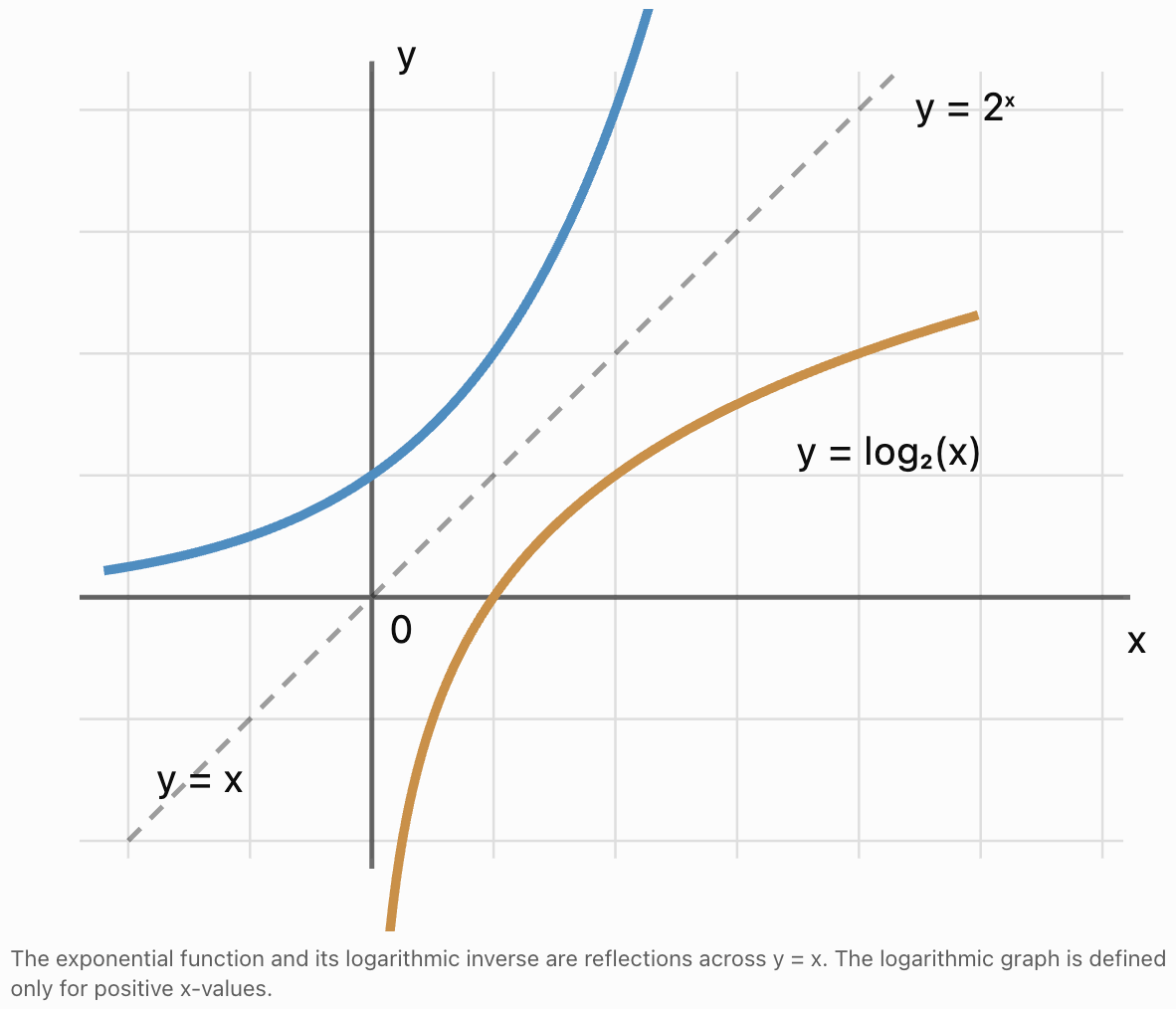
Consider the functions:
y = 2ˣ
and:
y = log₂(x)
These functions are inverses.
Their graphs are reflections of each other across the line:
y = x
Important Graph Features
For a base greater than 1:
Exponential function y = aˣ
-
Domain: all real numbers.
-
Range: y > 0.
-
Passes through (0, 1).
-
Has horizontal asymptote y = 0.
-
Increases from left to right.
Logarithmic function y = logₐ(x)
-
Domain: x > 0.
-
Range: all real numbers.
-
Passes through (1, 0).
-
Has vertical asymptote x = 0.
-
Increases from left to right.
If 0 < a < 1, both functions are decreasing rather than increasing.
Why the Logarithm of 1 Is Zero
For any valid base a:
a⁰ = 1
Therefore:
logₐ(1) = 0
Examples:
log₂(1) = 0
log₅(1) = 0
log₁₀(1) = 0
ln(1) = 0
This is one of the most useful basic logarithmic facts.
Why the Logarithm of the Base Is One
For any valid base a:
a¹ = a
Therefore:
logₐ(a) = 1
Examples:
log₂(2) = 1
log₃(3) = 1
log₁₀(10) = 1
ln(e) = 1
These two basic identities make many logarithmic expressions easy to evaluate.
Why Logarithms Cannot Have Zero or Negative Arguments
Consider:
log₂(0)
This asks:
"To what real power must 2 be raised to produce zero?"
No real exponent produces zero because:
2ˣ > 0
for every real x.
Therefore:
log₂(0) is undefined in the real numbers.
Similarly:
log₂(−8)
is undefined in the real numbers because a positive base raised to a real power always produces a positive result.
Domain Rule
For real logarithms:
logₐ(x) is defined only when x > 0, with a > 0 and a ≠ 1.
This restriction is essential when solving logarithmic equations.
Solving Simple Exponential Equations Using Logarithms
Logarithms are particularly useful when the exponent is unknown.
Worked Example
Solve:
2ˣ = 32
Since:
2⁵ = 32
x = 5
We can also write:
x = log₂(32)
x = 5
Worked Example: An Exponent That Is Not an Integer
Solve:
2ˣ = 10
There is no obvious whole-number exponent that produces 10.
Rewrite:
x = log₂(10)
Using a calculator or change of base:
x = log(10)/log(2)
x ≈ 3.322
Verification
2³·³²² ≈ 10
The result is reasonable because:
2³ = 8
2⁴ = 16
Therefore, x must lie between 3 and 4.
The Change-of-Base Formula
Scientific calculators usually provide LOG and LN keys, but not necessarily a dedicated key for every possible logarithmic base.
The change-of-base formula allows any logarithm to be evaluated using common or natural logarithms.
logₐ(x) = log(x)/log(a)
Equivalently:
logₐ(x) = ln(x)/ln(a)
These formulas apply when a > 0, a ≠ 1, and x > 0.
Worked Example
Evaluate:
log₃(20)
Using common logarithms:
log₃(20) = log(20)/log(3)
≈ 1.30103/0.47712
log₃(20) ≈ 2.727
Interpretation
3² = 9
3³ = 27
Since 20 lies between 9 and 27, its logarithm to base 3 lies between 2 and 3.
The calculated answer is reasonable.
Logarithms and Scientific Notation
Scientific notation expresses numbers using powers of 10.
For example:
450000 = 4.5 × 10⁵
The exponent tells us the order of magnitude.
Common logarithms help compare numbers of very different sizes.
Worked Example
Compare:
1000 and 1000000
Their common logarithms are:
log(1000) = 3
log(1000000) = 6
The difference is:
6 − 3 = 3
This means the larger number is 10³, or 1000 times, the smaller number.
Real-World Importance
Logarithmic thinking is useful when comparing:
-
Astronomical distances.
-
Microscopic measurements.
-
Large populations.
-
Scientific data.
-
Sound intensities.
-
Earthquake magnitudes.
Logarithmic Scales in Science
Some physical quantities vary over enormous ranges.
Logarithmic scales allow these quantities to be represented more conveniently.
Sound Intensity
Sound intensity level is measured in decibels.
A simplified formula is:
L = 10log₁₀(I/I₀)
where:
-
L = sound intensity level in decibels.
-
I = measured sound intensity.
-
I₀ = reference sound intensity.
If the intensity ratio is 1000:
L = 10log(1000)
= 10 × 3
L = 30 dB
This means the intensity is 1000 times the reference intensity.
Earthquake Magnitudes
Earthquake magnitude scales use logarithmic relationships.
An increase of one magnitude unit on a moment magnitude scale corresponds approximately to a tenfold increase in the measured seismic-wave amplitude under comparable conditions, while the energy released increases by roughly a factor of 32.
Logarithms make it possible to compare events with extremely different physical magnitudes.


Logarithms and Compound Interest
Exponential functions model repeated percentage growth.
For compound interest:
A = P(1 + r)ᵗ
where:
-
A = final amount.
-
P = initial amount.
-
r = interest rate per compounding period.
-
t = number of compounding periods.
Logarithms can determine how long it takes an investment to reach a target value.
Worked Example
An investment grows by 5% annually.
How many years will it take to double?
Step 1: Write the Model
A = P(1.05)ᵗ
For doubling:
2P = P(1.05)ᵗ
Step 2: Simplify
2 = 1.05ᵗ
Step 3: Use Logarithms
t = log(2)/log(1.05)
t ≈ 14.21 years
Interpretation
The investment takes approximately 14.21 years to double under the model.
If interest is credited only at the end of each complete year, the balance first reaches at least twice its initial value after 15 annual compounding periods.
Logarithms and Population Growth
Population growth can be represented using exponential functions.
For example:
P(t) = P₀ × 2^(t/5)
This model describes a population that doubles every five years.
Suppose the initial population is 1000.
How long will it take to reach 8000?
Step 1: Substitute
8000 = 1000 × 2^(t/5)
Step 2: Simplify
8 = 2^(t/5)
Step 3: Convert to Logarithmic Form
t/5 = log₂(8)
t/5 = 3
Step 4: Solve
t = 15 years
The population triples its number of doublings, not its population multiplier: three successive doublings multiply the initial population by 8.
Interpreting Logarithmic Values
A logarithmic value describes an exponent.
This gives useful information about the relationship between the argument and the base.
For bases greater than 1:
|
Argument |
Logarithm value |
|---|---|
|
x > 1 |
Positive |
|
x = 1 |
Zero |
|
0 < x < 1 |
Negative |
Examples
log₂(16) = 4
The argument is greater than 1, so the logarithm is positive.
log₂(1) = 0
The argument equals 1, so the logarithm is zero.
log₂(1/8) = −3
The argument is between 0 and 1, so the logarithm is negative.
For bases between 0 and 1, the sign pattern is reversed.
Common Mistakes
Confusing the base and the argument
In log₂(8), the base is 2 and the argument is 8.
Thinking a logarithm is a new type of multiplication
A logarithm determines an exponent.
Reversing exponential and logarithmic forms incorrectly
The correct relationship is:
aᵇ = c ⇔ logₐ(c) = b
Assuming logarithms must have positive values
Logarithms can be negative, zero, or positive.
Assuming logarithms can have negative arguments
Real logarithms require positive arguments.
Trying to calculate logₐ(0)
No valid positive base raised to a real exponent equals zero.
Confusing common and natural logarithms
Common logarithms use base 10.
Natural logarithms use base e.
Forgetting that the base cannot equal 1
The expression log₁(x) is not a valid logarithmic function.
Using the calculator incorrectly
For log₃(20), use log(20)/log(3), not log(20)/3.
Assuming log(a + b) = log(a) + log(b)
This is not a valid logarithm rule.
Failing to check whether an answer is reasonable
Estimate between familiar powers of the base before accepting a calculator result.
Key Terms
-
Logarithm: The exponent to which a base must be raised to produce a given positive number.
-
Base: The number repeatedly multiplied in an exponential expression.
-
Exponent: The power to which a base is raised.
-
Exponential Form: An equation written as aᵇ = c.
-
Logarithmic Form: An equivalent equation written as logₐ(c) = b.
-
Argument: The positive number inside a logarithmic expression.
-
Inverse Function: A function that reverses the action of another function.
-
Exponential Function: A function in which the variable appears in an exponent.
-
Logarithmic Function: A function that determines exponents for a fixed base.
-
Common Logarithm: A logarithm with base 10.
-
Natural Logarithm: A logarithm with base e.
-
Euler's Number (e): An irrational mathematical constant approximately equal to 2.71828.
-
Domain: The set of allowable input values for a function.
-
Range: The set of possible output values of a function.
-
Asymptote: A line that a graph approaches in a limiting sense.
-
Change-of-Base Formula: A formula used to rewrite logarithms using a different base.
-
Scientific Notation: A method of expressing numbers using powers of 10.
-
Order of Magnitude: A measure of numerical scale, often expressed using powers of 10.
-
Logarithmic Scale: A scale based on logarithms rather than equal numerical differences.
-
Decibel: A logarithmic unit used to express ratios of quantities such as sound intensity.
-
Exponential Growth: Growth in which a quantity increases by a constant multiplicative factor over equal intervals.
-
Exponential Decay: Decrease in which a quantity is multiplied by a constant factor between 0 and 1 over equal intervals.
-
Compound Interest: Interest calculated on an initial amount and previously accumulated interest.
-
Doubling Time: The time required for a growing quantity to become twice its initial value.
-
Continuous Growth: Growth modelled using exponential functions with base e.
-
Mathematical Model: A mathematical representation of a real-world process.
Key Takeaways
-
A logarithm is an exponent. It answers the question: "To what power must the base be raised to produce the argument?"
-
Logarithms and exponential functions are inverses of one another.
-
The fundamental relationship is aᵇ = c ⇔ logₐ(c) = b.
-
Converting between exponential and logarithmic forms is an essential skill.
-
The base of a real logarithm must be positive and cannot equal 1.
-
The argument of a real logarithm must be positive.
-
Logarithms can have positive, negative, zero, or fractional values.
-
The logarithm of 1 is always 0 for any valid base.
-
The logarithm of the base is always 1.
-
Common logarithms use base 10 and are often written as log(x).
-
Natural logarithms use base e and are written as ln(x).
-
Exponential and logarithmic graphs are reflections across the line y = x.
-
Logarithmic functions have domain x > 0 and range all real numbers.
-
The change-of-base formula allows logarithms with unfamiliar bases to be evaluated using a calculator.
-
Logarithms are useful for solving exponential equations with unknown exponents.
-
Logarithmic scales make it easier to compare quantities that vary across enormous ranges.
-
Common logarithms are especially useful in scientific notation and orders of magnitude.
-
Natural logarithms are fundamental in calculus and continuous growth models.
-
Logarithms are used in compound interest, population growth, sound intensity, earthquake measurement, and scientific modelling.
-
Understanding logarithms prepares students for logarithm laws, logarithmic equations, exponential modelling, and advanced calculus.
Check Your Understanding
Recall and Understanding
-
Define a logarithm in your own words.
-
Explain why logarithms and exponential functions are inverse operations.
-
Identify the base, argument, and logarithm value in log₄(64) = 3.
-
Explain the difference between a common logarithm and a natural logarithm.
-
Explain why log₂(0) and log₂(−4) are undefined in the real numbers.
Application
-
Convert 3⁵ = 243 into logarithmic form.
-
Convert log₅(125) = 3 into exponential form.
-
Evaluate log₂(128), log₃(1/9), and log₁₆(4).
-
Use the change-of-base formula to evaluate log₇(50), correct to three decimal places.
-
Solve 4ˣ = 30, giving your answer to three decimal places.
Analysis and Challenge
-
Explain why logₐ(1) = 0 and logₐ(a) = 1 for every valid logarithmic base.
-
Sketch y = 3ˣ and y = log₃(x) on the same coordinate system. Identify their intercepts, domains, ranges, asymptotes, and symmetry relationship.
-
An investment grows by 6% per year. Determine how long it will take to triple in value, assuming annual exponential growth.
-
A sound intensity is 100000 times a reference intensity. Use L = 10log(I/I₀) to calculate its sound intensity level in decibels.
-
A population is modelled by P(t) = 500e^(0.04t), where t is measured in years. Determine when the population will first reach 2000, and explain why natural logarithms are appropriate.
Final Summary
Logarithms provide a way to reverse exponential calculations.
While exponentiation determines the result of raising a base to a power, logarithms determine the exponent needed to produce a particular value.
The fundamental relationship is:
aᵇ = c ⇔ logₐ(c) = b
Understanding this relationship makes it possible to convert between exponential and logarithmic forms, evaluate logarithmic expressions, and solve equations involving unknown exponents.
Common logarithms use base 10, while natural logarithms use the mathematical constant e.
Logarithmic functions are inverses of exponential functions, and their graphs are reflections across the line y = x.
These ideas are essential in mathematics, science, engineering, finance, and many other fields.
The central idea is that logarithms transform questions about exponential growth and repeated multiplication into questions about exponents, making otherwise difficult calculations easier to understand and solve.
2. Graphing Logarithmic Functions
Learning outcomes
- I can sketch logarithmic graphs.
- I can identify domains and ranges.
- I can identify vertical asymptotes.
- I can compare logarithmic and exponential graphs.
- I can interpret logarithmic functions graphically.
Graphing Logarithmic Functions
Introduction to Logarithmic Graphs
Logarithmic functions are the inverses of exponential functions. While exponential functions describe how quantities change through repeated multiplication, logarithmic functions describe the exponent needed to produce a particular value.
A logarithmic function has the general form:
y = logₐ(x)
where:
-
a is the base.
-
a > 0 and a ≠ 1.
-
x is the input or argument.
-
y is the logarithmic value.
For example:
y = log₂(x)
asks: "To what power must 2 be raised to produce x?"
Understanding logarithmic graphs allows us to identify important features such as domains, ranges, intercepts, asymptotes, and transformations.
Logarithmic graphs are especially useful in science, engineering, finance, and situations involving quantities that vary over large numerical ranges.
The Basic Shape of a Logarithmic Graph
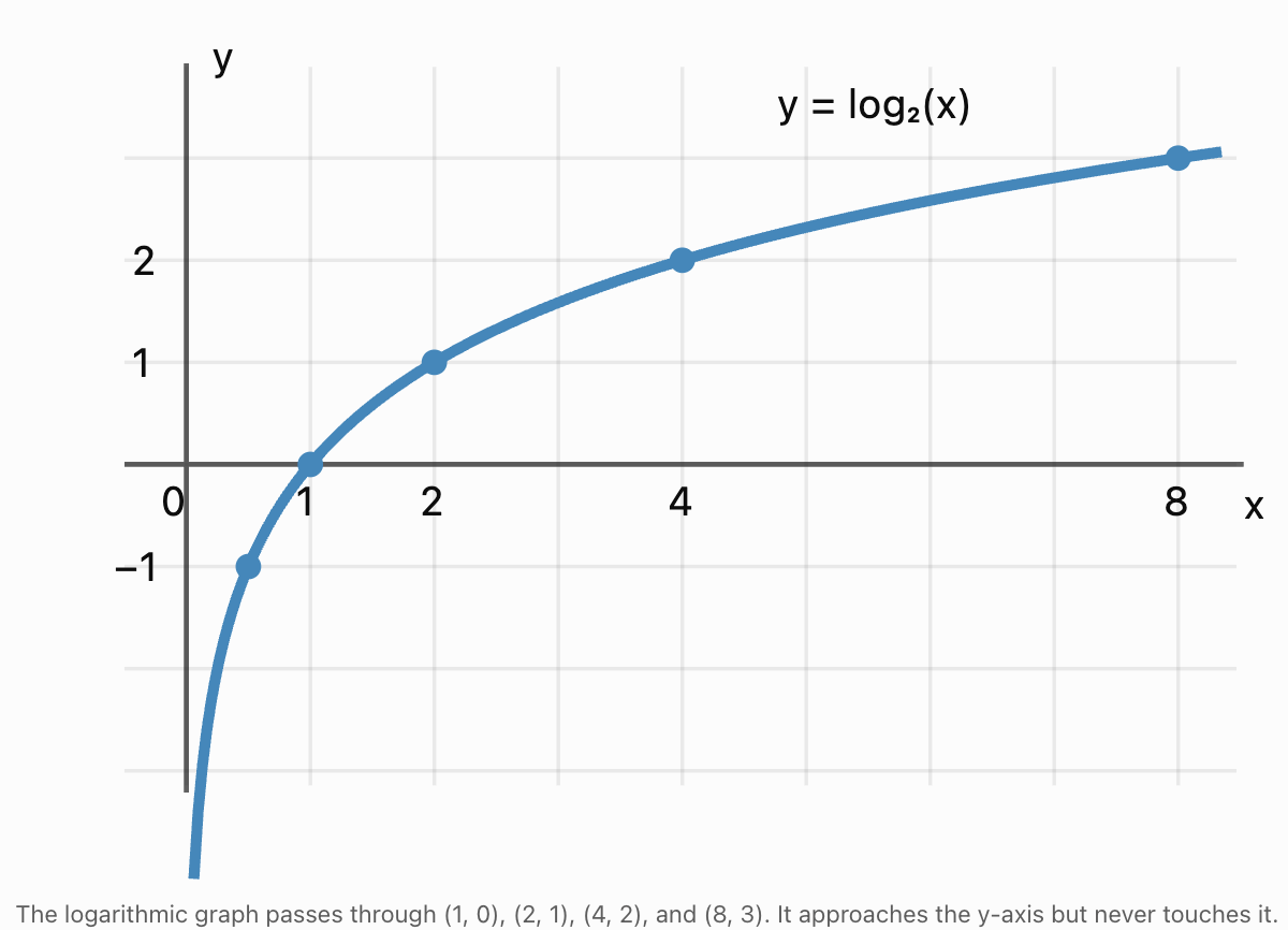
Consider:
y = log₂(x)
We can construct its graph by converting logarithmic expressions into exponential form.
Since:
y = log₂(x)
we can write:
x = 2ʸ
This allows us to generate points.
|
x |
y = log₂(x) |
|---|---|
|
1/8 |
−3 |
|
1/4 |
−2 |
|
1/2 |
−1 |
|
1 |
0 |
|
2 |
1 |
|
4 |
2 |
|
8 |
3 |
Plotting these coordinates produces a smooth curve that rises from left to right.
Important Observations
-
The graph exists only to the right of the y-axis.
-
It passes through (1, 0).
-
It increases as x increases.
-
It rises more slowly as x becomes larger.
-
It approaches the y-axis as x approaches zero from the positive side.
-
It continues indefinitely upward and downward.
These features are characteristic of logarithmic functions with bases greater than 1.
Domain of a Logarithmic Function
The domain is the set of all possible input values.
For:
y = logₐ(x)
the argument must be positive.
Therefore:
x > 0
The domain is:
(0, ∞)
This is true for every basic real logarithmic function with a valid base.
Why Must x Be Positive?
Consider:
y = log₂(x)
This is equivalent to:
x = 2ʸ
Since 2 raised to any real power is always positive, x cannot equal zero or be negative.
Therefore:
-
log₂(8) is defined.
-
log₂(1) is defined.
-
log₂(0.25) is defined.
-
log₂(0) is undefined in the real numbers.
-
log₂(−4) is undefined in the real numbers.
Worked Example
Determine the domain of:
f(x) = log₅(x)
The argument must be positive.
x > 0
Domain: (0, ∞)
Range of a Logarithmic Function
The range is the set of all possible output values.
For:
y = logₐ(x)
the logarithm can produce any real number.
For example:
log₂(1/8) = −3
log₂(1) = 0
log₂(8) = 3
The logarithmic value can become arbitrarily large or arbitrarily negative.
Therefore:
Range: (−∞, ∞)
Important Distinction
For the basic logarithmic function:
-
Domain: positive real numbers.
-
Range: all real numbers.
This is the reverse of the basic exponential function, whose domain is all real numbers and whose range is positive real numbers.
Vertical Asymptotes
An asymptote is a line that a graph approaches in a limiting sense.
For the basic logarithmic function:
y = logₐ(x)
the vertical asymptote is:
x = 0
This is the y-axis.
Understanding the Asymptote
For y = log₂(x), as x approaches zero from the right:
|
x |
log₂(x), approximately |
|---|---|
|
1 |
0 |
|
0.5 |
−1 |
|
0.25 |
−2 |
|
0.125 |
−3 |
|
0.01 |
−6.644 |
|
0.001 |
−9.966 |
As x approaches zero, the logarithm decreases without bound.
Mathematically:
lim(x → 0⁺) log₂(x) = −∞
The notation 0⁺ means approaching zero from positive values.
For bases between 0 and 1, the logarithmic function instead increases without bound as x approaches zero from the right.
Important Principle
The graph approaches its vertical asymptote but never reaches it.
The asymptote marks a boundary of the function's domain.
Intercepts of Logarithmic Graphs
An intercept is a point where a graph crosses an axis.
The x-Intercept
For:
y = logₐ(x)
the x-intercept occurs when:
y = 0
Therefore:
logₐ(x) = 0
Convert to exponential form:
x = a⁰
x = 1
Thus, every basic logarithmic function passes through:
(1, 0)
The y-Intercept
A y-intercept occurs when x = 0.
However:
logₐ(0)
is undefined.
Therefore, the basic logarithmic function has no y-intercept.
Summary
For y = logₐ(x):
-
x-intercept: (1, 0).
-
y-intercept: none.
-
Vertical asymptote: x = 0.
Increasing and Decreasing Logarithmic Functions
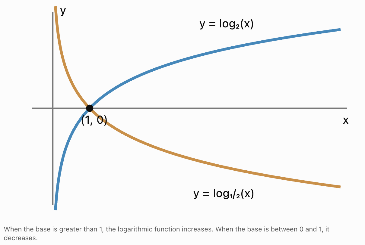
The shape of a logarithmic graph depends on its base.
Bases Greater Than 1
For:
a > 1
the graph increases from left to right.
Examples:
y = log₂(x)
y = log₃(x)
y = log₁₀(x)
As x increases, y increases.
Bases Between 0 and 1
For:
0 < a < 1
the graph decreases from left to right.
Examples:
y = log₁/₂(x)
y = log₁/₃(x)
As x increases, y decreases.
Comparing Values
|
x |
log₂(x) |
log₁/₂(x) |
|---|---|---|
|
1/4 |
−2 |
2 |
|
1/2 |
−1 |
1 |
|
1 |
0 |
0 |
|
2 |
1 |
−1 |
|
4 |
2 |
−2 |
Notice:
log₁/₂(x) = −log₂(x)
The two graphs are reflections across the x-axis.
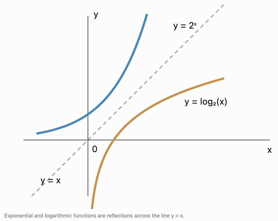
Comparing Logarithmic and Exponential Graphs
Logarithmic functions and exponential functions are inverses.
Consider:
y = 2ˣ
and:
y = log₂(x)
The exponential function converts exponents into values.
The logarithmic function converts values back into exponents.
Coordinate Relationships
For the exponential function:
|
x |
y = 2ˣ |
|---|---|
|
−2 |
1/4 |
|
−1 |
1/2 |
|
0 |
1 |
|
1 |
2 |
|
2 |
4 |
|
3 |
8 |
For its inverse:
|
x |
y = log₂(x) |
|---|---|
|
1/4 |
−2 |
|
1/2 |
−1 |
|
1 |
0 |
|
2 |
1 |
|
4 |
2 |
|
8 |
3 |
Notice that the coordinates are reversed.
For example:
The point (3, 8) lies on y = 2ˣ.
The point (8, 3) lies on y = log₂(x).
This is a defining property of inverse functions.
Reflection Across y = x
The graphs of a function and its inverse are reflections across the line:
y = x
Comparing Their Features
|
Feature |
Exponential: y = 2ˣ |
Logarithmic: y = log₂(x) |
|---|---|---|
|
Domain |
All real numbers |
x > 0 |
|
Range |
y > 0 |
All real numbers |
|
x-intercept |
None |
(1, 0) |
|
y-intercept |
(0, 1) |
None |
|
Asymptote |
y = 0 |
x = 0 |
|
Direction |
Increasing |
Increasing |
|
Inverse |
log₂(x) |
2ˣ |
The domain and range are exchanged, and the horizontal asymptote of the exponential function becomes a vertical asymptote for the logarithmic function.
Transformations of Logarithmic Functions
Like other functions, logarithmic graphs can be translated, reflected, and stretched.
The general transformed logarithmic function can be written:
y = A logₐ[B(x − h)] + k
where:
-
A controls vertical stretching and reflection.
-
a is the logarithmic base.
-
B controls horizontal stretching and reflection.
-
h determines the horizontal translation.
-
k determines the vertical translation.
The logarithm is defined only when its argument is positive:
B(x − h) > 0
The vertical asymptote occurs at:
x = h
provided A and B are nonzero and the base is valid.
Horizontal Translations
Consider:
y = log₂(x − 3)
This is the graph of y = log₂(x) shifted 3 units to the right.
Domain
The argument must be positive.
x − 3 > 0
x > 3
Domain:
(3, ∞)
Vertical Asymptote
The argument approaches zero when:
x − 3 = 0
x = 3
x-Intercept
Set y = 0.
log₂(x − 3) = 0
Convert to exponential form:
x − 3 = 2⁰
x − 3 = 1
x = 4
Therefore, the x-intercept is:
(4, 0)
Interpretation
The original graph passes through (1, 0).
After shifting 3 units right, it passes through (4, 0).
Horizontal Shifts to the Left
Consider:
y = log₃(x + 2)
This represents a shift 2 units to the left.
Domain
x + 2 > 0
x > −2
Vertical Asymptote
x = −2
x-Intercept
log₃(x + 2) = 0
x + 2 = 1
x = −1
The x-intercept is:
(−1, 0)
y-Intercept
Set x = 0.
y = log₃(2)
y ≈ 0.631
Therefore, the graph crosses the y-axis at approximately:
(0, 0.631)
Unlike the basic logarithmic graph, this transformed function has a y-intercept.
Vertical Translations
Consider:
y = log₂(x) + 3
The graph is shifted upward by 3 units.
Domain
The argument remains x.
Therefore:
x > 0
Range
The range remains all real numbers.
Vertical Asymptote
The asymptote remains:
x = 0
x-Intercept
Set y = 0.
log₂(x) + 3 = 0
log₂(x) = −3
x = 2⁻³
x = 1/8
Therefore, the x-intercept is:
(1/8, 0)
Important Principle
A vertical translation changes the output values but does not change the domain or vertical asymptote of a logarithmic function.
Reflections of Logarithmic Graphs
A negative coefficient outside a logarithm reflects its graph across the x-axis.
Consider:
y = −log₂(x)
The original graph increases.
The reflected graph decreases.
Important Features
-
Domain: x > 0.
-
Range: all real numbers.
-
Vertical asymptote: x = 0.
-
x-intercept: (1, 0).
-
Decreasing from left to right.
Reflection Across the y-Axis
Consider:
y = log₂(−x)
The argument must be positive.
−x > 0
x < 0
Therefore:
-
Domain: (−∞, 0).
-
Range: all real numbers.
-
Vertical asymptote: x = 0.
-
x-intercept: (−1, 0).
This graph is the reflection of y = log₂(x) across the y-axis.
Vertical Stretches and Compressions
Consider:
y = 3log₂(x)
Every output value of the original function is multiplied by 3.
For example:
|
x |
log₂(x) |
3log₂(x) |
|---|---|---|
|
1/2 |
−1 |
−3 |
|
1 |
0 |
0 |
|
2 |
1 |
3 |
|
4 |
2 |
6 |
The graph becomes steeper relative to the x-axis.
However, its domain and vertical asymptote remain unchanged.
Worked Example: Graphing a Transformed Logarithm
Sketch:
f(x) = 2log₃(x − 1) − 4
Identify the domain, range, vertical asymptote, and x-intercept.
Step 1: Identify Transformations
Starting with:
y = log₃(x)
the transformations are:
-
Shift right 1 unit.
-
Stretch vertically by a factor of 2.
-
Shift downward 4 units.
Step 2: Determine the Domain
The argument must be positive.
x − 1 > 0
x > 1
Domain:
(1, ∞)
Step 3: Determine the Range
A logarithmic function can produce every real output value.
Vertical stretching and translation do not change this.
Range: (−∞, ∞)
Step 4: Determine the Asymptote
Set the argument equal to zero.
x − 1 = 0
Vertical asymptote: x = 1
Step 5: Find the x-Intercept
Set y = 0.
0 = 2log₃(x − 1) − 4
4 = 2log₃(x − 1)
2 = log₃(x − 1)
Convert to exponential form:
x − 1 = 3²
x − 1 = 9
x = 10
Therefore:
x-intercept: (10, 0)
Step 6: Generate Points
|
x |
x − 1 |
log₃(x − 1) |
f(x) |
|---|---|---|---|
|
4/3 |
1/3 |
−1 |
−6 |
|
2 |
1 |
0 |
−4 |
|
4 |
3 |
1 |
−2 |
|
10 |
9 |
2 |
0 |
|
28 |
27 |
3 |
2 |
Final Interpretation
The graph increases from left to right, approaches the vertical asymptote x = 1, and crosses the x-axis at (10, 0).
It has no y-intercept because x = 0 lies outside its domain.
Finding the Domain of More Complicated Logarithmic Functions
For any real logarithmic function, the argument must be strictly positive.
This principle can be applied to more complicated expressions.
Worked Example: Linear Argument
Find the domain of:
f(x) = log₅(2x − 6)
Require:
2x − 6 > 0
2x > 6
x > 3
Domain:
(3, ∞)
Worked Example: Negative Coefficient
Find the domain of:
f(x) = ln(8 − 2x)
Require:
8 − 2x > 0
−2x > −8
Divide by −2 and reverse the inequality:
x < 4
Domain:
(−∞, 4)
Worked Example: Quadratic Argument
Find the domain of:
f(x) = log₂(x² − 9)
Require:
x² − 9 > 0
Factorise:
(x − 3)(x + 3) > 0
The product is positive when both factors are positive or both are negative.
Therefore:
x < −3 or x > 3
Domain:
(−∞, −3) ∪ (3, ∞)
This graph has two separate branches.
Its vertical asymptotes are x = −3 and x = 3, because the argument approaches zero from positive values at those boundaries.
This example demonstrates that more complicated logarithmic functions may have multiple domain intervals and vertical asymptotes.
Common and Natural Logarithmic Graphs
Two important logarithmic functions are:
y = log(x)
and:
y = ln(x)
In standard school notation:
log(x) = log₁₀(x)
ln(x) = logₑ(x)
Both graphs:
-
Have domain x > 0.
-
Have range all real numbers.
-
Pass through (1, 0).
-
Have vertical asymptote x = 0.
-
Increase from left to right.
However, they increase at different rates.
Comparing Values
|
x |
log₁₀(x), approximately |
ln(x), approximately |
|---|---|---|
|
0.1 |
−1 |
−2.303 |
|
1 |
0 |
0 |
|
2 |
0.301 |
0.693 |
|
10 |
1 |
2.303 |
|
100 |
2 |
4.605 |
For x > 1, ln(x) is greater than log₁₀(x).
For 0 < x < 1, ln(x) is more negative.
Interpreting Logarithmic Graphs
A logarithmic graph provides information about how an output changes as the input increases.
For:
y = log₂(x)
doubling the input increases the output by 1.
For example:
log₂(2) = 1
log₂(4) = 2
log₂(8) = 3
log₂(16) = 4
Each time x doubles, y increases by exactly 1.
General Pattern
For:
y = logₐ(x)
multiplying x by a increases the logarithm by 1.
This follows because:
logₐ(ax) = logₐ(x) + 1
for x > 0.
Why This Matters
Logarithmic functions compress large multiplicative changes into smaller additive changes.
This makes them useful for displaying data that spans several orders of magnitude.
Logarithmic Scales in Real-World Data
Logarithmic graphs are widely used in science and engineering.
Sound Intensity
Sound intensity level can be calculated using:
L = 10log₁₀(I/I₀)
where:
-
L = sound intensity level in decibels.
-
I = measured sound intensity.
-
I₀ = reference intensity.
If sound intensity increases by a factor of 10, the intensity level increases by 10 dB.
If it increases by a factor of 100, the intensity level increases by 20 dB.
Earthquake Magnitudes
Earthquake magnitude measurements use logarithmic relationships to represent enormous differences in seismic measurements.
Acidity and pH
The pH scale is defined by:
pH = −log₁₀(a_H⁺)
where a_H⁺ is the dimensionless activity of hydrogen ions. In dilute solutions, this is often approximated using hydrogen-ion concentration relative to 1 mol/L.
A tenfold increase in hydrogen-ion activity decreases pH by 1.
Computer Science
Logarithmic functions appear in algorithms, particularly when a problem can be repeatedly divided into smaller parts.
For example, binary search has logarithmic time complexity because each comparison eliminates approximately half the remaining possibilities.


Interpreting the Shape of a Logarithmic Graph
The graph of y = log₂(x) rises rapidly near x = 0 but increases more slowly for large x.
For example:
-
Increasing x from 1 to 2 raises y from 0 to 1.
-
Increasing x from 2 to 4 raises y from 1 to 2.
-
Increasing x from 4 to 8 raises y from 2 to 3.
-
Increasing x from 8 to 16 raises y from 3 to 4.
The horizontal increase required for the same vertical increase becomes progressively larger.
This behaviour is called diminishing growth in the rate of increase.
For bases greater than 1, the graph is increasing but concave downward.
Calculus Connection
For:
y = ln(x)
the derivative is:
dy/dx = 1/x
for x > 0.
As x increases, 1/x decreases.
This explains why the graph becomes less steep as x becomes larger.
For:
y = logₐ(x)
the derivative is:
dy/dx = 1/[x ln(a)]
For a > 1, this derivative is positive.
For 0 < a < 1, it is negative.
Thus, calculus confirms the increasing and decreasing behaviour observed graphically.
A Reliable Method for Sketching Logarithmic Graphs
When sketching a logarithmic function, use the following sequence.
-
Identify the base. Determine whether the function increases or decreases.
-
Find the domain. Set the logarithm's argument greater than zero and solve.
-
Find vertical asymptotes. Examine boundaries where the argument approaches zero from within the domain.
-
Find intercepts. Set y = 0 for x-intercepts and x = 0 for y-intercepts, where permitted.
-
Calculate convenient points. Choose arguments that are powers of the base.
-
Apply transformations. Account for shifts, stretches, and reflections.
-
Draw the curve. Sketch a smooth curve approaching its asymptote without crossing it.
-
Check the range and behaviour. Verify whether the function increases, decreases, or has multiple branches.
This approach works for many logarithmic functions encountered in secondary mathematics.
Common Mistakes
Assuming logarithmic functions accept all real inputs
The argument of a real logarithm must be positive.
Confusing the domain and range
For y = logₐ(x), the domain is x > 0 and the range is all real numbers.
Drawing a logarithmic graph through the y-axis
The basic logarithmic function has a vertical asymptote at x = 0.
Assuming every logarithmic graph increases
Logarithmic functions with bases between 0 and 1 decrease.
Confusing vertical and horizontal asymptotes
Basic exponential functions have horizontal asymptotes, while basic logarithmic functions have vertical asymptotes.
Forgetting transformations when identifying asymptotes
For y = log₂(x − 4), the vertical asymptote is x = 4, not x = 0.
Assuming all logarithmic functions pass through (1, 0)
This is true for basic logarithmic functions, but transformations can change the intercept.
Incorrectly interpreting horizontal translations
The function log₂(x − 3) shifts right 3 units, not left.
Forgetting to reverse an inequality when dividing by a negative number
This is especially important when finding the domain of functions such as ln(5 − x).
Confusing exponential and logarithmic coordinates
Inverse functions exchange their x- and y-coordinates.
Assuming logarithmic graphs are straight lines
Logarithmic functions are curved when plotted on ordinary linear axes.
Ignoring the context of a graph
A mathematical domain may need additional restrictions in a real-world situation.
Key Terms
-
Logarithmic Function: A function that determines the exponent required to produce a positive argument from a fixed base.
-
Exponential Function: A function in which the variable appears in the exponent.
-
Inverse Function: A function that reverses the action of another function.
-
Base: The fixed positive number, other than 1, used in a logarithmic expression.
-
Argument: The expression inside a logarithm.
-
Domain: The set of allowable input values.
-
Range: The set of possible output values.
-
Vertical Asymptote: A vertical line approached by a graph as the function values become unbounded near that line.
-
Horizontal Asymptote: A horizontal line approached by a graph as the input moves toward positive or negative infinity.
-
x-Intercept: A point where a graph crosses or touches the x-axis.
-
y-Intercept: A point where a graph crosses or touches the y-axis.
-
Increasing Function: A function whose outputs increase as its inputs increase.
-
Decreasing Function: A function whose outputs decrease as its inputs increase.
-
Transformation: A change to the position, orientation, or scale of a graph.
-
Horizontal Translation: A shift left or right.
-
Vertical Translation: A shift upward or downward.
-
Reflection: A transformation that flips a graph across a specified line.
-
Vertical Stretch: A transformation that multiplies the function's output values by a factor greater than 1.
-
Vertical Compression: A transformation that reduces the magnitude of the function's output values.
-
Common Logarithm: A logarithm with base 10.
-
Natural Logarithm: A logarithm with base e.
-
Logarithmic Scale: A scale that represents multiplicative changes using logarithmic values.
-
Order of Magnitude: A measure of numerical scale, commonly expressed using powers of 10.
-
Concavity: A description of how the slope of a graph changes.
-
Continuous Function: A function without breaks at points within its domain.
-
One-to-One Function: A function in which different inputs produce different outputs.
-
Reflection Across y = x: The graphical relationship between a function and its inverse.
-
Interval Notation: A method for expressing sets of real numbers using interval endpoints.
-
Graphical Interpretation: Using the features of a graph to understand mathematical relationships.
Key Takeaways
-
Logarithmic functions are the inverses of exponential functions.
-
The basic logarithmic function has the form y = logₐ(x), where a > 0 and a ≠ 1.
-
The argument of a real logarithm must always be positive.
-
The basic logarithmic function has domain (0, ∞).
-
Its range is all real numbers.
-
Every basic logarithmic graph passes through (1, 0).
-
Basic logarithmic functions have no y-intercept.
-
Their vertical asymptote is x = 0.
-
Logarithmic functions with bases greater than 1 increase from left to right.
-
Logarithmic functions with bases between 0 and 1 decrease from left to right.
-
Exponential and logarithmic graphs are reflections across y = x.
-
The domain and range of inverse functions are exchanged.
-
Horizontal translations change the domain and vertical asymptote of logarithmic functions.
-
Vertical translations change the output values but preserve the domain.
-
Reflections and stretches alter the shape or orientation of logarithmic graphs.
-
The domain of a transformed logarithmic function is determined by requiring its argument to be positive.
-
Convenient graphing points can be found by choosing arguments that are powers of the base.
-
Logarithmic graphs represent multiplicative relationships in a compressed form.
-
Logarithmic scales are useful for representing quantities spanning large numerical ranges.
-
Logarithmic functions appear in sound measurement, chemistry, earthquake analysis, computer science, and scientific modelling.
-
Graphical interpretation provides information about growth, change, intercepts, asymptotes, and mathematical restrictions.
Check Your Understanding
Recall and Understanding
-
Describe the general shape of y = log₂(x).
-
State the domain and range of a basic logarithmic function.
-
Explain why y = log₃(x) has a vertical asymptote at x = 0.
-
Describe the difference between logarithmic graphs with bases greater than 1 and bases between 0 and 1.
-
Explain how the graphs of y = 2ˣ and y = log₂(x) are related.
Application
-
Sketch y = log₃(x), identifying its domain, range, intercepts, and vertical asymptote.
-
Determine the domain and vertical asymptote of y = log₂(x − 5).
-
Find the x-intercept of y = log₄(x) + 2.
-
Sketch y = −log₂(x), explaining how it relates to y = log₂(x).
-
Determine the domain, range, and vertical asymptote of y = ln(7 − x).
Analysis and Challenge
-
A logarithmic graph passes through (2, 0) and (4, 1), and has a vertical asymptote at x = 1. Determine a function of the form y = logₐ(x − h) + k that satisfies these conditions.
-
Compare y = log₂(x) and y = log₄(x). Explain which graph increases more rapidly for x > 1 and justify your reasoning.
-
Find the domain and vertical asymptotes of y = log₃(x² − 16). Explain why the graph has two separate branches.
-
A sound intensity level is modelled by L = 10log₁₀(I/I₀). Explain graphically how the intensity level changes when the intensity is multiplied by 10, 100, and 1000.
-
Sketch y = −2log₃(x + 1) + 4. Identify its domain, range, vertical asymptote, intercepts, and transformations from y = log₃(x).
Final Summary
Logarithmic functions provide a graphical representation of inverse exponential relationships.
Their graphs have distinctive features, including restricted domains, unrestricted ranges, and vertical asymptotes.
The basic logarithmic function y = logₐ(x) passes through (1, 0) and is defined only for positive inputs.
When the base is greater than 1, the graph increases. When the base is between 0 and 1, the graph decreases.
Because logarithmic and exponential functions are inverses, their graphs are reflections across the line y = x.
Transformations allow logarithmic graphs to be shifted, stretched, compressed, and reflected. These transformations affect important features such as intercepts, domains, and asymptotes.
Logarithmic graphs are also valuable in real-world applications because they represent large multiplicative changes using comparatively small differences in output values.
The central principle is that understanding the domain, range, asymptote, intercepts, and transformations of a logarithmic function makes it possible to sketch and interpret its graph accurately without relying entirely on a calculator.
3. Properties of Logarithms
Learning outcomes
- I can apply the product rule.
- I can apply the quotient rule.
- I can apply the power rule.
- I can simplify logarithmic expressions.
- I can expand and condense logarithmic expressions.
Properties of Logarithms
Introduction to the Properties of Logarithms
Logarithms provide a powerful way to work with exponential expressions. While exponents describe repeated multiplication, logarithms determine the exponent required to produce a particular number.
The properties of logarithms allow complicated logarithmic expressions to be rewritten in simpler forms.
These properties are especially useful when:
-
Simplifying mathematical expressions.
-
Combining several logarithms into a single expression.
-
Expanding logarithmic expressions into separate terms.
-
Working with scientific and engineering formulas.
-
Analysing exponential growth and decay.
Three fundamental properties form the foundation of logarithmic algebra:
-
Product Rule: Multiplication becomes addition.
-
Quotient Rule: Division becomes subtraction.
-
Power Rule: Exponents become multipliers.
These rules follow directly from the laws of exponents.


Reviewing the Meaning of a Logarithm
Recall the relationship:
aᵇ = c ⇔ logₐ(c) = b
where:
-
a is the base.
-
b is the exponent.
-
c is the result.
For real logarithms:
-
a > 0.
-
a ≠ 1.
-
c > 0.
Example
Consider:
2⁵ = 32
The equivalent logarithmic statement is:
log₂(32) = 5
The logarithm tells us which exponent produces the argument.
This connection to exponents explains why logarithmic rules work.
The Product Rule
The product rule states that the logarithm of a product equals the sum of the logarithms of its factors.
logₐ(MN) = logₐ(M) + logₐ(N)
where:
-
a > 0 and a ≠ 1.
-
M > 0.
-
N > 0.
Understanding the Rule
Suppose:
2³ = 8
and:
2⁴ = 16
Multiplying:
8 × 16 = 128
Using exponent laws:
2³ × 2⁴ = 2⁷
Therefore:
log₂(128) = 7
But:
log₂(8) = 3
and:
log₂(16) = 4
So:
log₂(8 × 16) = log₂(8) + log₂(16)
7 = 3 + 4
The product rule works because multiplying powers with the same base adds their exponents.
Deriving the Product Rule
Let:
logₐ(M) = p
and:
logₐ(N) = q
Convert to exponential form:
M = aᵖ
N = aᑫ
Multiply:
MN = aᵖ × aᑫ
Using the exponent law:
aᵖ × aᑫ = a^(p+q)
Therefore:
MN = a^(p+q)
Convert back to logarithmic form:
logₐ(MN) = p + q
Substitute the original logarithms:
logₐ(MN) = logₐ(M) + logₐ(N)
This derivation shows that the product rule is a direct consequence of the laws of exponents.
Applying the Product Rule
Worked Example: Evaluating a Product
Evaluate:
log₂(4) + log₂(8)
Apply the product rule:
= log₂(4 × 8)
= log₂(32)
Since:
2⁵ = 32
Answer = 5
Worked Example: Combining Logarithms
Simplify:
log₃(5) + log₃(9)
Apply the product rule:
= log₃(5 × 9)
= log₃(45)
The result is a single logarithmic expression.
Worked Example: Three Logarithms
Condense:
log₂(3) + log₂(5) + log₂(7)
Combine the arguments:
= log₂(3 × 5 × 7)
= log₂(105)
The product rule can be extended to any finite number of positive factors.
Expanding Products
The product rule can also be used in reverse.
Consider:
log₅(6x)
Assuming x > 0:
log₅(6x) = log₅(6) + log₅(x)
This process is called expanding a logarithmic expression.
Worked Example
Expand:
log₂(12x)
Factorise:
12x = 3 × 4 × x
Apply the product rule:
log₂(12x) = log₂(3) + log₂(4) + log₂(x)
Since:
log₂(4) = 2
Answer = log₂(3) + 2 + log₂(x)
This expansion is valid for x > 0.
The Quotient Rule
The quotient rule states that the logarithm of a quotient equals the difference between the logarithms of the numerator and denominator.
logₐ(M/N) = logₐ(M) − logₐ(N)
where:
-
a > 0 and a ≠ 1.
-
M > 0.
-
N > 0.
Understanding the Rule
Consider:
2⁶ = 64
and:
2² = 4
Dividing:
64/4 = 16
Using exponent laws:
2⁶/2² = 2⁴
Therefore:
log₂(16) = 4
But:
log₂(64) = 6
and:
log₂(4) = 2
Thus:
log₂(64/4) = log₂(64) − log₂(4)
4 = 6 − 2
Division of powers with the same base corresponds to subtraction of exponents.
Deriving the Quotient Rule
Let:
logₐ(M) = p
logₐ(N) = q
Then:
M = aᵖ
N = aᑫ
Divide:
M/N = aᵖ/aᑫ
Using exponent laws:
M/N = a^(p−q)
Convert to logarithmic form:
logₐ(M/N) = p − q
Therefore:
logₐ(M/N) = logₐ(M) − logₐ(N)
Applying the Quotient Rule
Worked Example: Evaluating a Difference
Evaluate:
log₃(81) − log₃(9)
Apply the quotient rule:
= log₃(81/9)
= log₃(9)
Since:
3² = 9
Answer = 2
Worked Example: Combining Expressions
Condense:
log₅(20) − log₅(4)
= log₅(20/4)
= log₅(5)
Answer = 1
Worked Example: Expanding a Quotient
Expand:
log₂(x/8)
Assuming x > 0:
= log₂(x) − log₂(8)
Since:
log₂(8) = 3
Answer = log₂(x) − 3
The Power Rule
The power rule states that an exponent inside a logarithm can be moved in front as a multiplier.
logₐ(Mᵏ) = k logₐ(M)
where a > 0, a ≠ 1, M > 0, and k is any real number.
Understanding the Rule
Consider:
log₂(8³)
Since:
8 = 2³
then:
8³ = (2³)³
= 2⁹
Therefore:
log₂(8³) = 9
Using the power rule:
3log₂(8)
= 3 × 3
= 9
Both methods produce the same answer.
Deriving the Power Rule
Let:
logₐ(M) = p
Then:
M = aᵖ
Raise both sides to the power k:
Mᵏ = (aᵖ)ᵏ
Using exponent laws:
Mᵏ = a^(pk)
Convert to logarithmic form:
logₐ(Mᵏ) = pk
Since:
p = logₐ(M)
we obtain:
logₐ(Mᵏ) = k logₐ(M)
Applying the Power Rule
Worked Example: Expanding a Power
Expand:
log₃(x⁴)
For x > 0:
= 4log₃(x)
Worked Example: Evaluating an Expression
Evaluate:
3log₂(4)
Since:
log₂(4) = 2
3log₂(4) = 3 × 2
Answer = 6
Alternatively:
3log₂(4) = log₂(4³)
= log₂(64)
= 6
Worked Example: Fractional Exponents
Expand:
log₅(√x)
Assuming x > 0:
√x = x^(1/2)
Therefore:
log₅(√x) = log₅(x^(1/2))
= (1/2)log₅(x)
Worked Example: Negative Exponents
Simplify:
log₂(1/x³)
Assuming x > 0:
1/x³ = x⁻³
Therefore:
log₂(x⁻³) = −3log₂(x)
Answer = −3log₂(x)
Important Special Cases of the Power Rule
The power rule leads to several useful identities.
Logarithm of 1
Since:
a⁰ = 1
logₐ(1) = 0
Logarithm of the Base
Since:
a¹ = a
logₐ(a) = 1
Logarithm of a Power of the Base
logₐ(aᵏ) = k
For example:
log₃(3⁷) = 7
Exponential and Logarithmic Inverses
a^(logₐ(x)) = x
for x > 0.
These relationships make many logarithmic calculations easier.
Summary of the Three Main Rules
|
Rule |
Formula |
Operation |
|---|---|---|
|
Product |
logₐ(MN) = logₐ(M) + logₐ(N) |
Multiplication becomes addition |
|
Quotient |
logₐ(M/N) = logₐ(M) − logₐ(N) |
Division becomes subtraction |
|
Power |
logₐ(Mᵏ) = klogₐ(M) |
Exponents become multipliers |
For the product and quotient rules, M and N must be positive. For the power rule as written, M must be positive.
The logarithms must also use the same valid base.
Expanding Logarithmic Expressions
Expanding means rewriting a logarithm of a product, quotient, or power as separate logarithmic terms.
The usual approach is:
-
Identify products and quotients.
-
Apply the product and quotient rules.
-
Apply the power rule.
-
Simplify any logarithms that can be evaluated.
Worked Example: Product and Power
Expand completely:
log₂(8x³)
Assume x > 0.
Apply the product rule:
= log₂(8) + log₂(x³)
Apply the power rule:
= log₂(8) + 3log₂(x)
Since:
log₂(8) = 3
Answer = 3 + 3log₂(x)
Worked Example: Product, Quotient, and Power
Expand:
log₃(9x²/y⁴)
Assume x > 0 and y > 0.
Apply the quotient rule:
= log₃(9x²) − log₃(y⁴)
Apply the product rule:
= log₃(9) + log₃(x²) − log₃(y⁴)
Apply the power rule:
= 2 + 2log₃(x) − 4log₃
Final Answer:
2 + 2log₃(x) − 4log₃
Worked Example: Square Roots and Quotients
Expand:
ln(√x/y³)
Assume x > 0 and y > 0.
Rewrite the square root:
√x = x^(1/2)
Apply the quotient rule:
= ln(x^(1/2)) − ln(y³)
Apply the power rule:
= (1/2)ln(x) − 3ln
Handling Variables That May Be Negative
When expanding logarithms involving even powers, domain restrictions require special care.
For example:
log₂(x²)
is defined whenever x ≠ 0, including negative x.
Therefore, the expansion valid over the full real domain is:
log₂(x²) = 2log₂|x|
It is not generally correct to write 2log₂(x), because log₂(x) is undefined when x is negative.
Similarly:
ln(x²y⁴) = 2ln|x| + 4ln|y|
for x ≠ 0 and y ≠ 0.
Absolute values are unnecessary when the problem explicitly states that all variables are positive.
This distinction becomes especially important in advanced algebra and calculus.
Condensing Logarithmic Expressions
Condensing is the reverse of expanding.
It involves combining several logarithmic terms into a single logarithm.
The general procedure is:
-
Use the power rule to move coefficients into exponents.
-
Combine addition using the product rule.
-
Combine subtraction using the quotient rule.
-
Simplify the argument where possible.
Worked Example: Condensing Two Terms
Condense:
log₂(x) + log₂(5)
Apply the product rule:
= log₂(5x)
Valid for x > 0.
Worked Example: Coefficients and Subtraction
Condense:
3log₄(x) − 2log₄
Assume x > 0 and y > 0.
Apply the power rule:
= log₄(x³) − log₄(y²)
Apply the quotient rule:
= log₄(x³/y²)
Worked Example: Combining Three Terms
Condense:
2ln(x) + ln − 3ln(z)
Assume x, y, and z are positive.
Apply the power rule:
= ln(x²) + ln − ln(z³)
Apply the product rule:
= ln(x²y) − ln(z³)
Apply the quotient rule:
= ln(x²y/z³)
Multi-Step Expansion and Condensation
Some problems require all three rules.
Worked Example: Complete Expansion
Expand:
log₅[25x³√y/z²]
Assume x > 0, y > 0, and z > 0.
Step 1: Apply the Quotient Rule
= log₅(25x³√y) − log₅(z²)
Step 2: Apply the Product Rule
= log₅(25) + log₅(x³) + log₅(√y) − log₅(z²)
Step 3: Apply the Power Rule
= log₅(25) + 3log₅(x) + (1/2)log₅ − 2log₅(z)
Step 4: Evaluate the Constant
Since:
5² = 25
log₅(25) = 2
Final Answer
2 + 3log₅(x) + (1/2)log₅ − 2log₅(z)
Reverse Process
Starting with the expanded expression, the same rules can be applied in reverse to recover the original single logarithm.
This demonstrates that expansion and condensation are inverse algebraic processes.
Simplifying Logarithmic Expressions
Logarithmic expressions can often be simplified without a calculator.
Worked Example
Simplify:
log₂(16) + log₂(8) − log₂(4)
Apply the product and quotient rules:
= log₂[(16 × 8)/4]
= log₂(32)
Answer = 5
Worked Example
Simplify:
2log₃(9) − log₃(27)
Since:
log₃(9) = 2
log₃(27) = 3
we obtain:
2(2) − 3
Answer = 1
Alternatively:
= log₃(9²/27)
= log₃(3)
= 1
The Change-of-Base Formula
The change-of-base formula allows logarithms to be rewritten using a different base.
logₐ(x) = log(x)/log(a)
or:
logₐ(x) = ln(x)/ln(a)
where a > 0, a ≠ 1, and x > 0.
Worked Example
Evaluate:
log₄(20)
Using common logarithms:
log₄(20) = log(20)/log(4)
≈ 1.30103/0.60206
≈ 2.161
Why Change of Base Works
Let:
y = logₐ(x)
Then:
aʸ = x
Take the natural logarithm of both sides:
ln(aʸ) = ln(x)
Apply the power rule:
y ln(a) = ln(x)
Rearrange:
y = ln(x)/ln(a)
Therefore:
logₐ(x) = ln(x)/ln(a)
The change-of-base formula is itself an application of the power rule.
Simplifying Expressions with Different Bases
The product and quotient rules require logarithms with the same base.
However, the change-of-base formula can help when different bases appear.
Worked Example
Simplify:
log₂(8) + log₄(16)
Evaluate each logarithm:
log₂(8) = 3
log₄(16) = 2
Therefore:
Answer = 5
We cannot directly combine these terms using the product rule because their bases are different.
Another Example
Evaluate:
log₂(3) × log₃(8)
Using change of base:
log₂(3) = ln(3)/ln(2)
log₃(8) = ln(8)/ln(3)
Multiply:
= [ln(3)/ln(2)] × [ln(8)/ln(3)]
Cancel ln(3):
= ln(8)/ln(2)
= log₂(8)
Answer = 3
This illustrates how logarithmic properties can reveal relationships that are not immediately obvious.
Applying Logarithm Rules to Exponential Equations
Logarithmic properties are essential for solving exponential equations.
Worked Example
Solve:
3^(2x) = 50
Step 1: Take Logarithms
ln(3^(2x)) = ln(50)
Step 2: Apply the Power Rule
2x ln(3) = ln(50)
Step 3: Isolate x
x = ln(50)/[2ln(3)]
Step 4: Calculate
x ≈ 1.780
Verification
3^(2 × 1.780) ≈ 50
The result is reasonable.
Applying Logarithm Rules to Growth Models
Logarithms appear in many scientific models.
Consider exponential population growth:
P(t) = P₀e^(kt)
where:
-
P(t) is the population at time t.
-
P₀ is the initial population.
-
k is the continuous growth rate.
-
t is time.
Worked Example
A population follows:
P(t) = 500e^(0.08t)
Find when the population reaches 2000.
Step 1: Substitute
2000 = 500e^(0.08t)
Step 2: Divide
4 = e^(0.08t)
Step 3: Take Natural Logarithms
ln(4) = ln(e^(0.08t))
Step 4: Apply the Power Rule
ln(4) = 0.08t
Step 5: Solve
t = ln(4)/0.08
t ≈ 17.33
The population reaches 2000 after approximately 17.33 time units.


Logarithmic Properties in Science
The properties of logarithms are useful because they convert multiplication and powers into simpler algebraic operations.
Sound Intensity
Sound intensity level is calculated using:
L = 10log₁₀(I/I₀)
Applying the quotient rule:
L = 10[log₁₀(I) − log₁₀(I₀)]
when I and I₀ are expressed in the same positive units.
This demonstrates how a logarithmic ratio can be expanded into a difference.
Radioactive Decay
A simplified radioactive decay model is:
N(t) = N₀e^(−λt)
Taking natural logarithms:
ln[N(t)/N₀] = −λt
This form can be used to calculate decay constants or elapsed time.
Chemistry
The pH scale uses a logarithmic relationship:
pH = −log₁₀(a_H⁺)
where a_H⁺ is the dimensionless hydrogen-ion activity.
The power and quotient rules help analyse concentration ratios and changes in acidity.
Information Theory
Logarithms are used to quantify information.
For an event with probability p:
I = −log₂(p)
where I is the information content in bits.
For independent events with probabilities p and q:
−log₂(pq) = −log₂(p) − log₂(q)
Thus, the information associated with independent events adds.


Recognising Invalid Logarithm Rules
Not every algebraic operation has a corresponding logarithmic property.
The following statements are generally incorrect.
Incorrect:
logₐ(M + N) = logₐ(M) + logₐ(N)
Incorrect:
logₐ(M − N) = logₐ(M) − logₐ(N)
Incorrect:
logₐ(MN) = logₐ(M) × logₐ(N)
Numerical Counterexample
Consider:
log₂(2 + 2)
= log₂(4)
= 2
But:
log₂(2) + log₂(2)
= 1 + 1
= 2
These happen to agree, but this does not prove a general rule.
Choose a different example:
log₂(2 + 4)
= log₂(6)
≈ 2.585
However:
log₂(2) + log₂(4)
= 1 + 2
= 3
The values are different.
Therefore:
logₐ(M + N) ≠ logₐ(M) + logₐ(N)
in general.
The product rule applies to multiplication, not addition.
Choosing Between Expansion and Condensation
Different problems benefit from different forms.
|
Situation |
Recommended approach |
|---|---|
|
Simplifying a logarithm of a product |
Expand using the product rule |
|
Simplifying a logarithm of a quotient |
Expand using the quotient rule |
|
Removing an exponent from a logarithm |
Apply the power rule |
|
Combining several logarithmic terms |
Condense |
|
Solving an exponential equation |
Take logarithms and use the power rule |
|
Evaluating unfamiliar logarithmic bases |
Use change of base |
|
Simplifying a complex logarithmic fraction |
Expand or condense strategically |
|
Proving a logarithmic identity |
Transform one side using valid rules |
A useful strategy is to choose the form that makes the next algebraic step easiest.
Common Mistakes
Confusing multiplication with addition
The product rule applies to multiplication inside a logarithm, not addition.
Confusing division with subtraction
The quotient rule applies to a quotient inside a logarithm, not to subtraction inside the argument.
Applying the power rule incorrectly
The exponent becomes a multiplier outside the logarithm.
Using different bases in the product or quotient rule
The logarithms must have the same base before they can be combined directly.
Forgetting domain restrictions
Real logarithms require positive arguments.
Ignoring absolute values when expanding even powers
For example, logₐ(x²) = 2logₐ|x| for x ≠ 0.
Applying the product rule to negative factors
The real product rule requires both factors to be positive, even if their product is positive.
Forgetting to distribute coefficients
For example:
2[log(x) + log] = 2log(x) + 2log
Condensing before applying the power rule
It is often easier to move coefficients into exponents first.
Using logarithmic rules without checking equivalence
Algebraic transformations must preserve the original domain.
Rounding intermediate calculations too early
Retain sufficient precision until the final answer.
Key Terms
-
Logarithm: The exponent required to raise a given base to a specified positive value.
-
Base: The positive number, other than 1, used in a logarithmic expression.
-
Argument: The positive expression inside a logarithm.
-
Product Rule: The property that converts the logarithm of a product into a sum of logarithms.
-
Quotient Rule: The property that converts the logarithm of a quotient into a difference of logarithms.
-
Power Rule: The property that allows an exponent inside a logarithm to become a multiplier.
-
Expansion: Rewriting one logarithm as a sum or difference of simpler logarithms.
-
Condensation: Combining multiple logarithmic terms into one logarithm.
-
Logarithmic Expression: An algebraic expression containing logarithms.
-
Logarithmic Identity: A relationship involving logarithms that is valid throughout its stated domain.
-
Exponential Form: A mathematical statement written using a base raised to an exponent.
-
Logarithmic Form: An equivalent statement expressing the exponent as a logarithm.
-
Inverse Operation: An operation that reverses another operation.
-
Common Logarithm: A logarithm with base 10.
-
Natural Logarithm: A logarithm with base e.
-
Change-of-Base Formula: A formula that rewrites a logarithm using a different base.
-
Exponent Law: A mathematical rule describing operations involving powers.
-
Domain Restriction: A condition limiting allowable input values.
-
Absolute Value: The nonnegative magnitude of a real number.
-
Equivalent Expressions: Expressions that have equal values for every input in their common domain.
-
Exponential Equation: An equation containing a variable in an exponent.
-
Logarithmic Equation: An equation containing one or more logarithmic expressions.
-
Exponential Growth: Growth by a constant multiplicative factor over equal time intervals.
-
Exponential Decay: Decrease by a constant multiplicative factor over equal time intervals.
-
Continuous Growth: Exponential growth modelled using the constant e.
-
Mathematical Simplification: Rewriting an expression in a more useful equivalent form.
Key Takeaways
-
The three fundamental logarithm properties are the product rule, quotient rule, and power rule.
-
The product rule converts multiplication inside a logarithm into addition outside it.
-
The quotient rule converts division inside a logarithm into subtraction outside it.
-
The power rule converts an exponent inside a logarithm into a multiplier.
-
These rules follow directly from the laws of exponents.
-
Logarithms can be expanded into sums and differences of simpler logarithms.
-
Logarithmic expressions can also be condensed into a single logarithm.
-
Expansion and condensation are reverse processes.
-
Applying the power rule before condensing often simplifies the calculation.
-
Logarithmic properties can be used to evaluate expressions without a calculator.
-
The product and quotient rules require logarithms with the same base.
-
The arguments of real logarithms must be positive.
-
Absolute values may be necessary when expanding logarithms involving even powers of variables.
-
The change-of-base formula allows logarithms to be evaluated using common or natural logarithms.
-
Logarithmic rules are essential for solving exponential equations.
-
The properties of logarithms simplify mathematical models involving growth, decay, sound intensity, and scientific measurements.
-
There is no general logarithm rule that separates addition or subtraction inside an argument.
-
A valid logarithmic simplification must preserve mathematical equivalence and domain restrictions.
-
Mastering logarithmic properties provides the algebraic foundation for logarithmic equations, exponential modelling, and advanced calculus.
Check Your Understanding
Recall and Understanding
-
State the product, quotient, and power rules of logarithms.
-
Explain why the product rule follows from the laws of exponents.
-
Describe the difference between expanding and condensing logarithmic expressions.
-
Explain why logarithms must have the same base to use the product or quotient rule directly.
-
Explain why log₂(x²) cannot always be expanded as 2log₂(x) for every nonzero real x.
Application
-
Expand log₃(27x²), assuming x > 0.
-
Expand ln(x³/y²), assuming x > 0 and y > 0.
-
Condense 2log₅(x) + 3log₅
, assuming x > 0 and y > 0.
-
Simplify log₂(32) + log₂(4) − log₂(8).
-
Condense 3ln(a) − 2ln(b) + ln(c), assuming all variables are positive.
Analysis and Challenge
-
Expand log₂[8x⁴√y/z³] completely, assuming x, y, and z are positive.
-
Condense 2log₃(x) + (1/2)log₃
-
Prove the change-of-base formula using the power rule.
-
Solve 5^(3x−1) = 40 using logarithms, giving the answer to three decimal places.
-
A population follows P(t) = 1200e^(0.06t). Determine when it will reach 5000 and explain how the power rule is used in the solution.
Final Summary
The properties of logarithms provide a systematic way to simplify and manipulate expressions involving logarithmic functions.
The product rule transforms multiplication into addition.
The quotient rule transforms division into subtraction.
The power rule transforms exponents into multipliers.
These properties are derived from the laws of exponents and are fundamental to logarithmic algebra.
By applying the rules in reverse, several logarithmic terms can be combined into a single expression.
The same properties can be used to expand complicated logarithmic expressions into simpler components.
Logarithmic properties are also essential for solving exponential equations, working with growth and decay models, and interpreting scientific relationships.
Careful attention must be given to bases, positive arguments, domain restrictions, and valid algebraic transformations.
The central principle is that logarithms convert multiplicative and exponential relationships into additive and algebraic relationships, making complex expressions easier to simplify, analyse, and solve.
4. Changing Logarithm Bases
Learning outcomes
- I can apply the change-of-base formula.
- I can evaluate logarithms using technology.
- I can compare logarithms with different bases.
- I can simplify logarithmic calculations.
- I can solve practical logarithmic problems.
Changing Logarithm Bases
Introduction to Changing Logarithm Bases
Logarithms are useful for solving exponential equations, comparing quantities, and investigating mathematical relationships involving growth and decay.
However, logarithms can have many different bases.
For example:
-
log₂(8) = 3
-
log₃(81) = 4
-
log₅(125) = 3
-
log₁₀(1000) = 3
Some logarithms are easy to evaluate mentally because their arguments are familiar powers of their bases.
Others are more difficult.
Consider:
log₃(20)
This asks:
"To what power must 3 be raised to produce 20?"
Since:
3² = 9
and:
3³ = 27
the answer must lie between 2 and 3.
However, determining its exact numerical value requires a more powerful method.
The change-of-base formula allows logarithms with any valid base to be rewritten using another valid base.
This makes logarithms easier to evaluate, compare, simplify, and apply to practical problems.

Reviewing Logarithmic Notation
Recall that logarithms are inverse operations of exponentiation.
The relationship is:
aˣ = b ⇔ logₐ(b) = x
where:
-
a is the base.
-
b is the argument.
-
x is the exponent.
For real logarithms:
-
a > 0.
-
a ≠ 1.
-
b > 0.
Example
Consider:
2⁴ = 16
The equivalent logarithmic expression is:
log₂(16) = 4
The logarithm determines the exponent needed to produce the argument.
An Unfamiliar Logarithm
Consider:
log₂(10)
Since:
2³ = 8
and:
2⁴ = 16
we know:
3 < log₂(10) < 4
But how can we calculate a more precise answer?
The change-of-base formula provides the solution.
The Change-of-Base Formula
The change-of-base formula states:
logₐ(b) = log꜀(b)/log꜀(a)
where a and c are positive bases other than 1, and b > 0.
This means that a logarithm can be rewritten using any other valid logarithmic base.
Two particularly useful forms are:
logₐ(b) = log(b)/log(a)
and:
logₐ(b) = ln(b)/ln(a)
Here:
-
log represents the common logarithm, with base 10.
-
ln represents the natural logarithm, with base e.
Both formulas produce exactly the same result.
Example
To calculate:
log₃(20)
we can write:
log₃(20) = log(20)/log(3)
or:
log₃(20) = ln(20)/ln(3)
Both expressions evaluate to approximately:
2.727
Why the Change-of-Base Formula Works
The change-of-base formula follows directly from the definition of logarithms and the power rule.
Derivation
Let:
x = logₐ(b)
Convert to exponential form:
aˣ = b
Take the natural logarithm of both sides:
ln(aˣ) = ln(b)
Apply the power rule:
x ln(a) = ln(b)
Divide both sides by ln(a):
x = ln(b)/ln(a)
Since:
x = logₐ(b)
we obtain:
logₐ(b) = ln(b)/ln(a)
The same reasoning works with common logarithms:
logₐ(b) = log(b)/log(a)
Important Conclusion
The change-of-base formula is not an approximation.
It is an exact mathematical identity.
Approximation occurs only when the result is rounded to a decimal value.
Evaluating Logarithms Using Common Logarithms
Most scientific calculators include a LOG key.
This usually calculates logarithms to base 10.
Worked Example
Evaluate:
log₂(10)
Step 1: Apply Change of Base
log₂(10) = log(10)/log(2)
Step 2: Evaluate
log(10) = 1
log(2) ≈ 0.301030
Therefore:
log₂(10) ≈ 1/0.301030
log₂(10) ≈ 3.322
Step 3: Check Reasonableness
We know:
2³ = 8
2⁴ = 16
Since 10 lies between 8 and 16, the exponent must lie between 3 and 4.
The calculated value is reasonable.
Evaluating Logarithms Using Natural Logarithms
Natural logarithms use base e, where:
e ≈ 2.71828
The natural logarithm is written:
ln(x)
Worked Example
Evaluate:
log₅(18)
Step 1: Apply Change of Base
log₅(18) = ln(18)/ln(5)
Step 2: Calculate
ln(18) ≈ 2.890372
ln(5) ≈ 1.609438
Therefore:
log₅(18) ≈ 2.890372/1.609438
log₅(18) ≈ 1.796
Step 3: Verify
Since:
5¹ = 5
5² = 25
the logarithm of 18 to base 5 must lie between 1 and 2.
The answer is consistent with this estimate.
Common Logarithms and Natural Logarithms
Common and natural logarithms are especially useful because calculators and mathematical software support them directly.
|
Feature |
Common logarithm |
Natural logarithm |
|---|---|---|
|
Base |
10 |
e ≈ 2.71828 |
|
Notation |
log(x) |
ln(x) |
|
Calculator key |
LOG |
LN |
|
Example |
log(100) = 2 |
ln(e²) = 2 |
|
Common applications |
Scientific notation, logarithmic scales |
Calculus, continuous growth and decay |
Which Should You Use?
For ordinary numerical calculations, either is suitable.
For example:
log₇(25) = log(25)/log(7)
and:
log₇(25) = ln(25)/ln(7)
Both give approximately:
1.654
Natural logarithms are often preferred in calculus and continuous growth models because they work naturally with exponential functions involving e.
Using a Scientific Calculator
A scientific calculator can evaluate logarithms with unfamiliar bases using the change-of-base formula.
Example: Calculate log₄(30)
Enter:
log(30) ÷ log(4)
or:
ln(30) ÷ ln(4)
The result is:
log₄(30) ≈ 2.453
Some calculators also provide a logarithm template that allows the base and argument to be entered directly.
Calculator Procedure
-
Identify the base and argument.
-
Enter LOG or LN of the argument.
-
Divide by LOG or LN of the base.
-
Evaluate.
-
Round only the final answer to the required precision.
Important Calculator Rule
Use the same logarithmic base in the numerator and denominator.
Correct:
log(30)/log(4)
Correct:
ln(30)/ln(4)
Incorrect:
log(30)/ln(4)
The final expression does not represent log₄(30).
Evaluating Logarithms with Technology
Graphing calculators, spreadsheets, and mathematical software can also evaluate logarithms.
Spreadsheet Examples
In many spreadsheet applications:
=LOG(20,3)
calculates log₃(20).
Alternatively:
=LN(20)/LN(3)
produces the same result.
For common logarithms:
=LOG10(1000)
returns 3.
For natural logarithms:
=LN(EXP(2))
returns 2, apart from possible floating-point rounding.
Benefits of Technology
Technology is especially useful when:
-
The logarithmic base is unfamiliar.
-
The argument is not a simple power.
-
High numerical precision is required.
-
Many logarithmic calculations must be performed.
-
Logarithmic values are used in graphs or models.
However, students should still understand what the result means and whether it is reasonable.
Comparing Logarithms with Different Bases
The value of a logarithm depends on both its base and its argument.
For example:
log₂(16) = 4
log₄(16) = 2
log₁₆(16) = 1
The argument remains 16, but the logarithmic value changes because the base changes.
Why Does This Happen?
Consider the equivalent exponential equations:
2⁴ = 16
4² = 16
16¹ = 16
Different bases require different exponents to produce the same number.
Numerical Comparison
|
Argument x |
log₂(x) |
log₃(x) |
log₁₀(x) |
|---|---|---|---|
|
1 |
0 |
0 |
0 |
|
2 |
1 |
0.631 |
0.301 |
|
4 |
2 |
1.262 |
0.602 |
|
8 |
3 |
1.893 |
0.903 |
|
16 |
4 |
2.524 |
1.204 |
|
32 |
5 |
3.155 |
1.505 |
For x > 1, a smaller base greater than 1 produces a larger logarithmic value.
For 0 < x < 1, the ordering reverses.
Comparing Logarithmic Graphs
Consider:
y = log₂(x)
y = log₃(x)
y = log₁₀(x)
All three functions:
-
Have domain x > 0.
-
Have range all real numbers.
-
Pass through (1, 0).
-
Have vertical asymptote x = 0.
-
Increase from left to right.
However, they increase at different rates.
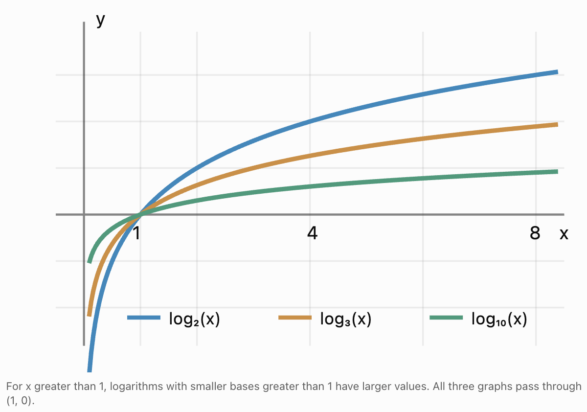
Comparing Bases Between Zero and One
Logarithms can also have bases between 0 and 1.
For example:
y = log₁/₂(x)
Since:
(1/2)⁻¹ = 2
we know:
log₁/₂(2) = −1
Unlike logarithmic functions with bases greater than 1, these functions decrease from left to right.
Change-of-Base Example
Evaluate:
log₁/₂(8)
Apply change of base:
log₁/₂(8) = ln(8)/ln(1/2)
Since:
ln(1/2) = −ln(2)
and:
ln(8) = 3ln(2)
we obtain:
log₁/₂(8) = −3
Important Observation
The change-of-base formula works for all valid positive bases other than 1, including bases between 0 and 1.
Useful Identities Involving Different Bases
Changing bases reveals several important logarithmic identities.
Reciprocal Identity
logₐ(b) = 1/logᵦ(a)
for positive a and b other than 1.
Derivation
Using change of base:
logₐ(b) = ln(b)/ln(a)
Also:
logᵦ(a) = ln(a)/ln(b)
These expressions are reciprocals.
Worked Example
Evaluate:
log₂(8) × log₈(2)
Since:
log₂(8) = 3
and:
log₈(2) = 1/3
their product is:
1
Chain Identity
Another useful relationship is:
logₐ(b) × logᵦ(c) = logₐ(c)
where all bases and arguments are valid.
Derivation
logₐ(b) = ln(b)/ln(a)
logᵦ(c) = ln(c)/ln(b)
Multiply:
[ln(b)/ln(a)] × [ln(c)/ln(b)]
Cancel ln(b):
= ln(c)/ln(a)
Therefore:
logₐ(b) × logᵦ(c) = logₐ(c)
Worked Example
Simplify:
log₂(5) × log₅(32)
Using the chain identity:
= log₂(32)
Since:
2⁵ = 32
Answer = 5
Simplifying Calculations by Choosing a Convenient Base
Although any valid base can be used, some choices make calculations easier.
Example
Evaluate:
log₄(64)
Using change of base:
log₄(64) = log₂(64)/log₂(4)
Since:
log₂(64) = 6
log₂(4) = 2
Answer = 3
This is simpler than evaluating decimal logarithms.
Another Example
Evaluate:
log₉(27)
Rewrite using base 3:
log₉(27) = log₃(27)/log₃(9)
= 3/2
Answer = 1.5
General Strategy
When the base and argument are powers of a common number, changing to that common base may produce an exact answer.
Logarithms with Powers as Bases
The change-of-base formula can simplify logarithms whose bases are powers.
Consider:
logₐᵏ(b)
Using change of base:
logₐᵏ(b) = ln(b)/ln(aᵏ)
Apply the power rule:
= ln(b)/[kln(a)]
Therefore:
logₐᵏ(b) = (1/k)logₐ(b)
provided a > 0, a ≠ 1, and k ≠ 0.
Worked Example
Simplify:
log₈(64)
Since:
8 = 2³
and:
64 = 2⁶
we obtain:
log₈(64) = 6/3
Answer = 2
Another Example
Simplify:
log₂₅(125)
Since:
25 = 5²
and:
125 = 5³
we obtain:
log₂₅(125) = 3/2
Answer = 1.5
Solving Exponential Equations Using Change of Base
One of the most important applications of the change-of-base formula is solving equations where the variable appears in an exponent.
Worked Example
Solve:
3ˣ = 20
Step 1: Convert to Logarithmic Form
x = log₃(20)
Step 2: Apply Change of Base
x = ln(20)/ln(3)
Step 3: Evaluate
x ≈ 2.995732/1.098612
x ≈ 2.727
Verification
3² = 9
3³ = 27
Since 20 lies between 9 and 27, the exponent must lie between 2 and 3.
The answer is reasonable.
Solving Multi-Step Exponential Equations
Worked Example
Solve:
5^(2x−1) = 40
Step 1: Take Logarithms
ln[5^(2x−1)] = ln(40)
Step 2: Apply the Power Rule
(2x − 1)ln(5) = ln(40)
Step 3: Divide
2x − 1 = ln(40)/ln(5)
Step 4: Solve for x
2x = 1 + ln(40)/ln(5)
x = [1 + ln(40)/ln(5)]/2
Step 5: Calculate
x ≈ 1.646
Interpretation
The exponent is approximately:
2(1.646) − 1 ≈ 2.292
Raising 5 to this power gives approximately 40.
Practical Application: Compound Interest
Compound interest can be modelled by:
A = P(1 + r/n)^(nt)
where:
-
A = final amount.
-
P = initial principal.
-
r = annual interest rate as a decimal.
-
n = number of compounding periods per year.
-
t = time in years.
Logarithms allow us to solve for time.
Worked Example
An investment of $5000 earns 6% annual interest, compounded monthly.
How long will it take to grow to $8000?
Step 1: Write the Formula
8000 = 5000(1 + 0.06/12)^(12t)
Step 2: Simplify
1.6 = 1.005^(12t)
Step 3: Take Natural Logarithms
ln(1.6) = 12t ln(1.005)
Step 4: Solve
t = ln(1.6)/[12ln(1.005)]
Step 5: Calculate
t ≈ 7.85 years
Interpretation
The investment reaches $8000 after approximately 7.85 years according to the continuous-time solution of the monthly-compounding formula.
Because interest is actually credited monthly, the balance first reaches at least $8000 after 95 complete monthly compounding periods, or approximately 7.92 years.
Practical Application: Population Growth
Suppose a population increases by 4% each year.
The model is:
P(t) = P₀(1.04)ᵗ
Find the time required for the population to double.
Step 1: Set Up the Equation
2P₀ = P₀(1.04)ᵗ
Divide by P₀:
2 = 1.04ᵗ
Step 2: Apply Logarithms
t = log₁.₀₄(2)
Step 3: Change Base
t = ln(2)/ln(1.04)
Step 4: Calculate
t ≈ 17.67 years
Interpretation
The population takes approximately 17.67 years to double under this exponential growth model.


Practical Application: Radioactive Decay
Radioactive decay is commonly modelled by:
N(t) = N₀e^(−λt)
where:
-
N(t) = amount remaining.
-
N₀ = initial amount.
-
λ = decay constant.
-
t = time.
The half-life is the time required for half the original material to remain.
Worked Example
A radioactive substance has a decay constant of 0.035 per year.
Find its half-life.
Step 1: Set Up the Equation
N(t) = N₀/2
Therefore:
1/2 = e^(−0.035t)
Step 2: Take Natural Logarithms
ln(1/2) = −0.035t
Step 3: Solve
t = ln(1/2)/(−0.035)
Since:
ln(1/2) = −ln(2)
we obtain:
t = ln(2)/0.035
Step 4: Calculate
t ≈ 19.80 years
Natural logarithms are especially convenient for models involving the base e.
Practical Application: Sound Intensity
Sound intensity levels are measured in decibels.
The formula is:
L = 10log₁₀(I/I₀)
where:
-
L = intensity level in decibels.
-
I = measured intensity.
-
I₀ = reference intensity.
Worked Example
A sound has an intensity 500 times the reference intensity.
Calculate its intensity level.
Step 1: Substitute
L = 10log₁₀(500)
Step 2: Evaluate
log₁₀(500) ≈ 2.69897
Therefore:
L ≈ 10 × 2.69897
L ≈ 26.99 dB
Interpretation
The sound intensity level is approximately 27.0 dB above the reference level.
Logarithmic scales make large intensity ratios easier to express and compare.
Practical Application: pH
The pH scale measures acidity using a logarithmic relationship.
pH = −log₁₀(a_H⁺)
where a_H⁺ represents dimensionless hydrogen-ion activity.
In dilute solutions, hydrogen-ion activity is often approximated using concentration relative to 1 mol/L.
Worked Example
Suppose the hydrogen-ion activity is:
a_H⁺ = 2.5 × 10⁻⁴
Calculate the pH.
Step 1: Substitute
pH = −log₁₀(2.5 × 10⁻⁴)
Step 2: Apply the Product Rule
pH = −[log₁₀(2.5) + log₁₀(10⁻⁴)]
Step 3: Simplify
log₁₀(10⁻⁴) = −4
Therefore:
pH = −[log₁₀(2.5) − 4]
Step 4: Calculate
log₁₀(2.5) ≈ 0.39794
pH ≈ −(0.39794 − 4)
pH ≈ 3.60
This example combines logarithmic properties with scientific measurement.


Practical Application: Computer Science
Logarithms are important in computer science because some algorithms repeatedly divide a problem into smaller parts.
For example, binary search repeatedly halves the number of possibilities.
Suppose a sorted collection contains 1024 items.
Since:
1024 = 2¹⁰
a binary search can locate an item or establish its absence using at most approximately 11 comparisons, depending on the exact implementation and how comparisons are counted.
The logarithm:
log₂(1024) = 10
describes the number of times 1024 can be halved to reach 1.
Worked Example
A data structure contains 5000 items.
Estimate:
log₂(5000)
Using change of base:
log₂(5000) = ln(5000)/ln(2)
≈ 12.288
This indicates that the number of halving stages grows much more slowly than the number of items.
Choosing the Best Logarithmic Base
Different problems may benefit from different logarithmic bases.
|
Situation |
Convenient base |
|---|---|
|
Powers of 2 |
Base 2 |
|
Powers of 3 |
Base 3 |
|
Powers of 10 |
Base 10 |
|
Scientific notation |
Base 10 |
|
Continuous growth and decay |
Base e |
|
Compound interest calculations |
Base 10 or e |
|
Calculator evaluation |
Base 10 or e |
|
Binary search and information theory |
Base 2 |
|
Simplifying powers of a common number |
That common base |
The change-of-base formula allows us to choose whichever base makes a calculation easiest.
A Strategy for Logarithmic Calculations
When solving a logarithmic problem:
-
Identify the base and argument.
-
Check that the logarithm is defined.
-
Determine whether the answer can be found using familiar powers.
-
Look for common bases that simplify the expression.
-
Apply the change-of-base formula when necessary.
-
Use logarithmic properties to simplify expressions.
-
Evaluate using appropriate technology.
-
Check the answer against nearby powers or the original equation.
-
Round only at the final stage.
-
Interpret the result in the context of the problem.
This approach helps reduce errors and encourages efficient mathematical reasoning.
Common Mistakes
Reversing the numerator and denominator
Correct:
logₐ(b) = log(b)/log(a)
The argument goes in the numerator, and the original base goes in the denominator.
Using different logarithm bases in the numerator and denominator
Correct:
ln(b)/ln(a)
Incorrect:
ln(b)/log(a)
Confusing common and natural logarithms
LOG normally means base 10, while LN means base e.
Assuming changing the base changes the value
The change-of-base formula produces an equivalent expression with exactly the same value.
Using an invalid logarithmic base
The base must be positive and cannot equal 1.
Using zero or negative arguments
Real logarithms require positive arguments.
Ignoring bases between zero and one
These are valid logarithmic bases and produce decreasing logarithmic functions.
Rounding too early
Intermediate rounding can reduce the accuracy of multi-step calculations.
Failing to estimate the answer
Comparing the argument with nearby powers provides a useful reasonableness check.
Confusing logarithmic growth with exponential growth
Exponential functions increase multiplicatively, while logarithmic functions describe the exponents associated with those changes.
Using an inappropriate real-world model
Exponential models depend on assumptions such as constant proportional growth or decay.
Key Terms
-
Logarithm: The exponent required to raise a given base to a positive argument.
-
Base: The positive number, other than 1, used in a logarithmic expression.
-
Argument: The positive number or expression inside a logarithm.
-
Change-of-Base Formula: A mathematical identity used to express a logarithm using a different base.
-
Common Logarithm: A logarithm with base 10.
-
Natural Logarithm: A logarithm with base e.
-
Euler's Number (e): An irrational constant approximately equal to 2.71828.
-
Exponential Form: A mathematical expression involving a base raised to a power.
-
Logarithmic Form: An equivalent expression that identifies the exponent.
-
Inverse Function: A function that reverses another function.
-
Power Rule: A logarithmic property that converts an exponent into a multiplier.
-
Product Rule: A logarithmic property that converts multiplication into addition.
-
Quotient Rule: A logarithmic property that converts division into subtraction.
-
Equivalent Expressions: Expressions that produce the same values throughout their common domain.
-
Reciprocal Identity: A relationship connecting logₐ(b) and logᵦ(a).
-
Chain Identity: A relationship in which logₐ(b) × logᵦ(c) = logₐ(c).
-
Scientific Calculator: A calculator capable of evaluating advanced mathematical functions.
-
Numerical Approximation: A decimal value close to an exact mathematical result.
-
Precision: The level of detail or number of significant digits in a numerical result.
-
Exponential Equation: An equation containing a variable in an exponent.
-
Compound Interest: Interest calculated on an initial principal and previously accumulated interest.
-
Exponential Growth: Growth by a constant multiplicative factor over equal time intervals.
-
Exponential Decay: Decrease by a constant multiplicative factor over equal time intervals.
-
Decay Constant: A parameter describing the rate of continuous exponential decay.
-
Half-Life: The time required for a decaying quantity to decrease to half its original value.
-
Logarithmic Scale: A scale that represents multiplicative changes through logarithmic values.
-
Decibel: A logarithmic unit used to describe ratios such as sound intensity.
-
Binary Search: An algorithm that repeatedly divides a sorted search interval approximately in half.
-
Mathematical Model: A mathematical representation of a real-world system.
-
Verification: The process of checking whether a calculated answer satisfies the original conditions.
Key Takeaways
-
The change-of-base formula allows logarithms with any valid base to be rewritten using another valid base.
-
The general formula is logₐ(b) = log꜀(b)/log꜀(a).
-
Common logarithms and natural logarithms are especially useful for calculator evaluations.
-
The formulas logₐ(b) = log(b)/log(a) and logₐ(b) = ln(b)/ln(a) are mathematically equivalent.
-
The change-of-base formula follows from the power rule of logarithms.
-
Changing the base does not change the numerical value of a logarithm.
-
Logarithms with different bases can be compared using common or natural logarithms.
-
For x > 1, smaller bases greater than 1 produce larger logarithmic values.
-
Logarithms with bases between zero and one decrease as their arguments increase.
-
The reciprocal identity connects logarithms with reversed bases and arguments.
-
The chain identity allows products of logarithms with related bases to be simplified.
-
Choosing a convenient common base can produce exact answers without a calculator.
-
The change-of-base formula is useful for solving exponential equations with unfamiliar bases.
-
Technology allows logarithms to be evaluated accurately, but mathematical estimation remains important.
-
Logarithms are used to calculate growth times, doubling times, and decay rates.
-
Natural logarithms are especially convenient for models involving continuous exponential change.
-
Logarithmic scales simplify comparisons involving large numerical ranges.
-
Applications include compound interest, population growth, radioactive decay, sound intensity, chemistry, and computer science.
-
A complete solution should include the appropriate formula, correct substitution, accurate calculation, and a meaningful interpretation.
-
Understanding how to change logarithmic bases makes logarithms more flexible and provides an important foundation for advanced algebra, scientific modelling, and calculus.
Check Your Understanding
Recall and Understanding
-
State the change-of-base formula.
-
Explain why the change-of-base formula works.
-
Describe the difference between common logarithms and natural logarithms.
-
Explain why log₂(16) and log₄(16) have different values.
-
Explain why a calculator can evaluate logarithms with unfamiliar bases using only LOG or LN.
Application
-
Evaluate log₃(25), correct to three decimal places.
-
Use change of base to calculate log₇(40).
-
Simplify log₄(64) using a convenient common base.
-
Evaluate log₁/₃(27).
-
Solve 4ˣ = 75, giving your answer to three decimal places.
Analysis and Challenge
-
Prove that logₐ(b) = 1/logᵦ(a), stating the necessary restrictions.
-
Simplify log₂(7) × log₇(49) without using a calculator.
-
An investment grows by 5% annually. Determine how long it will take to double in value.
-
A radioactive substance follows N(t) = 800e^(−0.025t). Determine when only 200 units remain.
-
A sound intensity is 2500 times a reference intensity. Calculate its sound intensity level in decibels and explain how the logarithmic scale represents this large ratio.
Final Summary
Changing logarithmic bases is an essential technique in algebra and mathematical modelling.
The change-of-base formula allows logarithms with unfamiliar bases to be expressed using common or natural logarithms.
This makes it possible to evaluate logarithms accurately using scientific calculators, spreadsheets, and mathematical software.
The formula also reveals important relationships between logarithms with different bases, including reciprocal and chain identities.
By choosing convenient bases, complicated logarithmic expressions can often be simplified into exact values.
Changing bases is especially useful when solving exponential equations, calculating growth and decay times, and interpreting logarithmic scales in science and engineering.
The central principle is that the value of a logarithm does not depend on the notation used to calculate it. By changing to a convenient base, we can make difficult logarithmic calculations simpler without changing their mathematical meaning.
5. Applications of Logarithms
Learning outcomes
- I can interpret pH values.
- I can interpret the Richter scale.
- I can interpret sound intensity levels.
- I can analyse logarithmic scales.
- I can solve real-world logarithmic problems.
Applications of Logarithms
Introduction to Logarithms in the Real World
Logarithms are used throughout science, engineering, technology, and mathematics to describe quantities that vary over extremely large ranges.
Many natural phenomena involve multiplicative relationships rather than simple additive changes.
For example:
-
The concentration of hydrogen ions in a solution can vary by factors of millions.
-
Earthquakes can produce seismic waves with vastly different amplitudes.
-
Sound intensities can differ by trillions of times.
-
Populations and investments may grow exponentially.
-
Astronomical distances and brightness measurements can span enormous ranges.
Representing these quantities on ordinary linear scales can be difficult.
Logarithmic scales solve this problem by converting multiplicative changes into additive changes.
This allows scientists to compare very large and very small quantities using manageable numerical values.
Three important applications of logarithms are:
-
The pH scale in chemistry.
-
Earthquake magnitude scales in geology.
-
The decibel scale in acoustics.


Understanding Logarithmic Scales
A logarithmic scale represents quantities using logarithms rather than their original numerical values.
Consider the numbers:
1, 10, 100, 1000, 10000
On a linear scale, the numerical differences are:
9, 90, 900, 9000
On a base-10 logarithmic scale, the corresponding values are:
0, 1, 2, 3, 4
This is because:
log₁₀(1) = 0
log₁₀(10) = 1
log₁₀(100) = 2
log₁₀(1000) = 3
log₁₀(10000) = 4
Each increase of 1 on the logarithmic scale represents multiplication by 10 in the original quantity.
Comparing Linear and Logarithmic Scales
|
Original quantity |
log₁₀(quantity) |
|---|---|
|
1 |
0 |
|
10 |
1 |
|
100 |
2 |
|
1000 |
3 |
|
10000 |
4 |
|
100000 |
5 |
|
1000000 |
6 |
A logarithmic scale compresses an enormous range of quantities into a relatively small range of values.
Why Logarithmic Scales Are Useful
Logarithmic scales are particularly useful when:
-
Quantities span several orders of magnitude.
-
Multiplicative differences are more meaningful than additive differences.
-
Exponential relationships need to be represented graphically.
-
Very small and very large measurements must be compared.
-
Scientists need to identify proportional changes.
For example, an increase from 10 to 100 is a tenfold increase.
An increase from 1000 to 10000 is also a tenfold increase.
On a logarithmic scale, both changes occupy the same distance.
Linear Versus Logarithmic Graphs
On a linear graph, equal distances represent equal numerical differences.
On a logarithmic graph, equal distances represent equal multiplicative ratios.
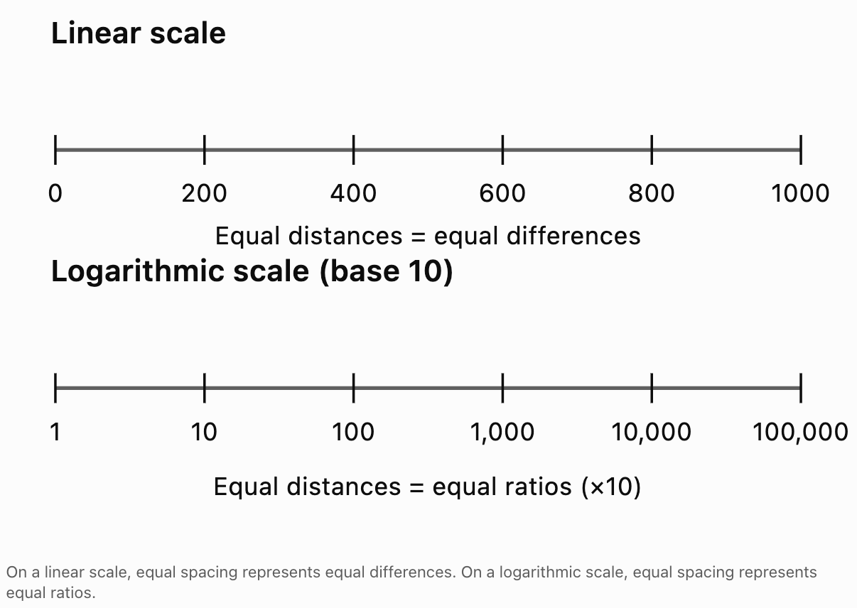
The pH Scale
The pH scale is used to describe the acidity or alkalinity of aqueous solutions.
It is based on the activity of hydrogen ions.
The mathematical definition is:
pH = −log₁₀(a_H⁺)
where:
-
pH is the acidity measure.
-
a_H⁺ is the dimensionless activity of hydrogen ions.
For dilute aqueous solutions, hydrogen-ion activity is often approximated using hydrogen-ion concentration relative to 1 mol/L.
This gives the familiar school-level approximation:
pH ≈ −log₁₀([H⁺]/(1 mol/L))
where [H⁺] is the hydrogen-ion concentration.
Understanding pH Values
At approximately 25°C:
-
pH below 7 indicates an acidic solution.
-
pH of 7 indicates a neutral solution.
-
pH above 7 indicates a basic or alkaline solution.
These familiar boundaries apply to typical dilute aqueous solutions at 25°C. The pH of neutrality changes with temperature, and pH values can fall outside the usual 0–14 range.

Why pH Is Logarithmic
The pH scale is logarithmic because hydrogen-ion activity can vary enormously.
Consider two solutions:
Solution A:
a_H⁺ = 0.01
Solution B:
a_H⁺ = 0.0001
For Solution A:
pH = −log₁₀(0.01)
pH = 2
For Solution B:
pH = −log₁₀(0.0001)
pH = 4
The difference is only 2 pH units.
However, the hydrogen-ion activity differs by a factor of:
0.01/0.0001 = 100
Solution A has 100 times the hydrogen-ion activity of Solution B.
This is why small differences in pH can represent large chemical differences.
Interpreting pH Differences
For two solutions with pH values pH₁ and pH₂:
a₁/a₂ = 10^(pH₂ − pH₁)
where a₁ and a₂ are their hydrogen-ion activities.
Examples
|
Difference in pH |
Hydrogen-ion activity ratio |
|---|---|
|
1 unit |
10 times |
|
2 units |
100 times |
|
3 units |
1000 times |
|
4 units |
10000 times |
|
5 units |
100000 times |
A decrease of 1 pH unit represents a tenfold increase in hydrogen-ion activity.
A decrease of 2 pH units represents a hundredfold increase.
Worked Example: Calculating pH
A solution has a hydrogen-ion activity of:
a_H⁺ = 3.2 × 10⁻⁴
Calculate its pH.
Step 1: Write the Formula
pH = −log₁₀(a_H⁺)
Step 2: Substitute
pH = −log₁₀(3.2 × 10⁻⁴)
Step 3: Apply Logarithm Rules
pH = −[log₁₀(3.2) + log₁₀(10⁻⁴)]
Since:
log₁₀(10⁻⁴) = −4
we obtain:
pH = −[log₁₀(3.2) − 4]
Step 4: Calculate
log₁₀(3.2) ≈ 0.50515
pH ≈ −(0.50515 − 4)
pH ≈ 3.49
Interpretation
The solution is acidic.
Worked Example: Comparing Two pH Values
A solution has pH 3.
Another solution has pH 6.
How many times greater is the hydrogen-ion activity in the first solution?
Step 1: Find the pH Difference
6 − 3 = 3
Step 2: Calculate the Ratio
Ratio = 10³
Ratio = 1000
Final Answer
The solution with pH 3 has 1000 times greater hydrogen-ion activity than the solution with pH 6.
Important Distinction
A solution with pH 3 is not simply twice as acidic as a solution with pH 6.
The pH scale is logarithmic, not linear.
Worked Example: Finding Hydrogen-Ion Activity
A solution has:
pH = 5.5
Calculate its hydrogen-ion activity.
Step 1: Write the Formula
pH = −log₁₀(a_H⁺)
Step 2: Substitute
5.5 = −log₁₀(a_H⁺)
Step 3: Rearrange
−5.5 = log₁₀(a_H⁺)
Step 4: Convert to Exponential Form
a_H⁺ = 10⁻⁵·⁵
Step 5: Calculate
a_H⁺ ≈ 3.16 × 10⁻⁶
This illustrates how logarithms can be reversed to determine the original physical quantity.
Applications of pH
The pH scale is important in:
-
Drinking water treatment.
-
Agriculture and soil management.
-
Aquatic ecosystems.
-
Food production.
-
Human physiology.
-
Industrial chemistry.
-
Environmental monitoring.
For example, aquatic organisms may be sensitive to changes in water pH because these changes affect chemical equilibria and the availability or toxicity of dissolved substances.


Earthquake Magnitude and the Richter Scale
Earthquakes produce seismic waves that travel through the Earth.
Seismographs record these waves, allowing scientists to estimate earthquake magnitude.
The original Richter scale, developed in 1935, was a logarithmic local-magnitude scale based on seismic-wave amplitudes recorded under specified conditions.
Modern seismology more commonly uses the moment magnitude scale (Mw), especially for large earthquakes.
Both use logarithmic relationships, but they are not identical measurement systems.


Understanding the Richter Scale
A simplified model of the Richter scale is:
M = log₁₀(A/A₀)
where:
-
M is the earthquake magnitude.
-
A is a measured seismic-wave amplitude.
-
A₀ is a reference amplitude.
Actual Richter local-magnitude calculations also account for factors such as the distance between the earthquake and the recording station.
Meaning of the Scale
An increase of one magnitude unit corresponds to a tenfold increase in the relevant corrected seismic-wave amplitude.
For example:
-
Magnitude 4 to magnitude 5: amplitude increases by a factor of 10.
-
Magnitude 4 to magnitude 6: amplitude increases by a factor of 100.
-
Magnitude 4 to magnitude 7: amplitude increases by a factor of 1000.
Important Distinction
Earthquake magnitude is not the same as earthquake damage.
Damage depends on factors such as:
-
Earthquake depth.
-
Distance from the epicentre.
-
Local geology.
-
Building construction.
-
Duration of shaking.
-
Population density.
Worked Example: Comparing Earthquake Amplitudes
Earthquake A has magnitude 4.5.
Earthquake B has magnitude 6.5.
Compare their seismic-wave amplitudes using the simplified logarithmic relationship.
Step 1: Calculate the Magnitude Difference
ΔM = 6.5 − 4.5
ΔM = 2
Step 2: Calculate the Amplitude Ratio
Amplitude ratio = 10^ΔM
= 10²
= 100
Final Answer
The relevant corrected seismic-wave amplitude of Earthquake B is 100 times that of Earthquake A.
Worked Example: Finding a Magnitude Difference
One earthquake produces a corrected seismic-wave amplitude 500 times that of another earthquake.
Find the difference in magnitude.
Step 1: Write the Relationship
ΔM = log₁₀(A₂/A₁)
Step 2: Substitute
ΔM = log₁₀(500)
Step 3: Calculate
ΔM ≈ 2.699
Final Answer
The magnitude difference is approximately 2.70 units.
This shows that a very large amplitude difference can correspond to a relatively small numerical magnitude difference.
Earthquake Energy and Magnitude
Earthquake magnitude is also related to the energy released.
For moment magnitude, an increase of one magnitude unit corresponds approximately to an energy increase by a factor of:
10¹·⁵ ≈ 31.6
A commonly used approximate energy relationship is:
log₁₀(E) ≈ 1.5Mw + 4.8
where:
-
E is seismic energy in joules.
-
Mw is moment magnitude.
This is an approximate relationship, not an exact energy measurement for every earthquake.
Comparing Earthquake Energy
For two earthquakes:
E₂/E₁ ≈ 10^[1.5(M₂ − M₁)]
Worked Example
Compare the approximate energy released by magnitude 5 and magnitude 7 earthquakes.
Step 1: Find the Magnitude Difference
7 − 5 = 2
Step 2: Apply the Energy Relationship
E₂/E₁ ≈ 10^(1.5 × 2)
= 10³
= 1000
Final Answer
A magnitude 7 earthquake releases approximately 1000 times as much seismic energy as a magnitude 5 earthquake.
Important Principle
A tenfold increase in corrected seismic-wave amplitude per magnitude unit is not the same as a tenfold increase in released energy.
The energy relationship is much steeper.
Sound Intensity and Decibels
Sound is produced by vibrations that transfer energy through a medium.
Sound intensity measures the sound power passing through a unit area.
The SI unit of sound intensity is:
W/m²
The human auditory system can respond to sound intensities spanning an enormous range.
A logarithmic scale makes these values easier to compare.
The sound intensity level is measured in decibels (dB).


The Decibel Formula
Sound intensity level is calculated using:
L = 10log₁₀(I/I₀)
where:
-
L is sound intensity level in decibels.
-
I is measured sound intensity.
-
I₀ is reference sound intensity.
A common reference intensity in air is:
I₀ = 10⁻¹² W/m²
Understanding the Formula
If:
I = I₀
then:
L = 10log₁₀(1)
Since:
log₁₀(1) = 0
L = 0 dB
Zero decibels does not mean no sound.
It means the intensity equals the chosen reference intensity.
Understanding Decibel Differences
Because decibels use a logarithmic scale, equal increases in decibels represent equal multiplicative changes in intensity.
|
Increase in sound intensity level |
Intensity multiplier |
|---|---|
|
3 dB |
Approximately 2 |
|
10 dB |
10 |
|
20 dB |
100 |
|
30 dB |
1000 |
|
40 dB |
10000 |
|
60 dB |
1000000 |
A 10 dB increase represents a tenfold increase in sound intensity.
A 20 dB increase represents a hundredfold increase.
A 30 dB increase represents a thousandfold increase.
Perceived loudness is different from physical intensity and depends on frequency, duration, and human hearing.
Worked Example: Calculating Sound Intensity Level
A sound has an intensity of:
I = 10⁻⁶ W/m²
Calculate its intensity level.
Step 1: Write the Formula
L = 10log₁₀(I/I₀)
Step 2: Substitute
L = 10log₁₀(10⁻⁶/10⁻¹²)
Step 3: Simplify
10⁻⁶/10⁻¹² = 10⁶
Therefore:
L = 10log₁₀(10⁶)
Step 4: Evaluate
log₁₀(10⁶) = 6
L = 10 × 6
L = 60 dB
Worked Example: Comparing Two Sounds
Sound A has an intensity level of 40 dB.
Sound B has an intensity level of 70 dB.
How many times greater is the intensity of Sound B?
Step 1: Find the Difference
ΔL = 70 − 40
ΔL = 30 dB
Step 2: Rearrange the Decibel Relationship
ΔL = 10log₁₀(I₂/I₁)
Therefore:
I₂/I₁ = 10^(ΔL/10)
Step 3: Substitute
I₂/I₁ = 10^(30/10)
= 10³
= 1000
Final Answer
Sound B has 1000 times the intensity of Sound A.
Worked Example: Finding Sound Intensity
A sound intensity level is 85 dB.
Calculate its intensity using:
I₀ = 10⁻¹² W/m²
Step 1: Write the Formula
85 = 10log₁₀(I/I₀)
Step 2: Divide by 10
8.5 = log₁₀(I/I₀)
Step 3: Convert to Exponential Form
I/I₀ = 10⁸·⁵
Step 4: Rearrange
I = I₀ × 10⁸·⁵
Step 5: Substitute
I = 10⁻¹² × 10⁸·⁵
I = 10⁻³·⁵
I ≈ 3.16 × 10⁻⁴ W/m²
Comparing pH, Earthquake Magnitude, and Decibels
All three applications use logarithms, but they represent different physical relationships.
|
Feature |
pH |
Earthquake magnitude |
Sound intensity level |
|---|---|---|---|
|
Main quantity |
Hydrogen-ion activity |
Seismic measurement |
Sound intensity |
|
Typical logarithm base |
10 |
10 |
10 |
|
Basic relationship |
pH = −log₁₀(a_H⁺) |
M = log₁₀(A/A₀), simplified |
L = 10log₁₀(I/I₀) |
|
Change of 1 unit |
Tenfold change in hydrogen-ion activity |
Tenfold change in corrected amplitude |
Intensity multiplied by 10^0.1 ≈ 1.259 |
|
Change of 10 units |
Ten-billionfold activity ratio |
Ten-billionfold amplitude ratio |
Tenfold intensity ratio |
The same logarithmic principle appears in each system, but the coefficients and physical meanings differ.
A General Formula for Logarithmic Scales
Many logarithmic scales can be expressed as:
S = k log₁₀(Q/Q₀)
where:
-
S is the logarithmic scale value.
-
k is a scale factor.
-
Q is the measured quantity.
-
Q₀ is a reference quantity.
Comparing Two Measurements
For two values:
S₁ = k log₁₀(Q₁/Q₀)
S₂ = k log₁₀(Q₂/Q₀)
Subtract:
S₂ − S₁ = k log₁₀(Q₂/Q₁)
Therefore:
ΔS = k log₁₀(Q₂/Q₁)
Rearranging:
Q₂/Q₁ = 10^(ΔS/k)
This formula is useful for comparing quantities on logarithmic scales.
Examples
For a decibel intensity scale:
k = 10
Therefore:
I₂/I₁ = 10^(ΔL/10)
For the simplified earthquake amplitude relationship:
k = 1
Therefore:
A₂/A₁ = 10^ΔM
For pH, the negative sign reverses the direction of the relationship.
Logarithmic Graphs in Scientific Data
Logarithmic axes are useful when data covers a wide range of values.
Scientists may use:
-
Linear-linear graphs.
-
Semilogarithmic graphs.
-
Log-log graphs.
Linear-Linear Graphs
Both axes use ordinary linear scales.
These are useful for relationships involving additive changes.
Semilogarithmic Graphs
One axis is logarithmic.
These are useful for exponential growth or decay.
For example:
y = Ae^(kx)
Taking natural logarithms:
ln = ln(A) + kx
This is a straight-line relationship between ln and x.
Log-Log Graphs
Both axes are logarithmic.
These are useful for power-law relationships.
For example:
y = Cxⁿ
Taking logarithms:
log = log(C) + nlog(x)
A graph of log against log(x) is a straight line with slope n.


Worked Example: Exponential Growth on a Semilogarithmic Graph
A bacterial population follows:
P(t) = 500e^(0.3t)
where t is measured in hours.
Step 1: Take Natural Logarithms
ln[P(t)] = ln[500e^(0.3t)]
Step 2: Apply Logarithmic Properties
ln[P(t)] = ln(500) + ln[e^(0.3t)]
Therefore:
ln[P(t)] = ln(500) + 0.3t
Step 3: Interpret
A graph of ln(P) against t is a straight line.
Its:
-
Slope is 0.3 per hour.
-
Vertical intercept is ln(500).
This makes logarithmic graphs useful for identifying exponential relationships in experimental data.
Worked Example: A Power Law on a Log-Log Graph
Suppose a physical quantity follows:
F = Cr²
where C is a positive constant.
Take logarithms:
log(F) = log(Cr²)
Apply the product rule:
log(F) = log(C) + log(r²)
Apply the power rule:
log(F) = log(C) + 2log(r)
Therefore, a graph of log(F) against log(r) is a straight line with slope 2.
This is a powerful technique for identifying mathematical relationships from data.
Other Applications of Logarithms
Logarithms appear in many additional fields.
Astronomy
The astronomical magnitude system uses logarithms to compare the apparent brightness of celestial objects.
A difference of 5 magnitudes corresponds to a brightness ratio of 100.
Brighter objects have smaller numerical magnitudes.
Finance
Logarithms help determine how long investments take to reach a target value.
For example:
A = P(1 + r)ᵗ
Taking logarithms:
t = log(A/P)/log(1 + r)
Population Growth
Exponential growth models can be solved using logarithms.
For:
P(t) = P₀e^(kt)
the time required to reach a target population is:
t = ln[P(t)/P₀]/k
for k ≠ 0.
Computer Science
Logarithms describe the efficiency of algorithms such as binary search.
Repeatedly halving a search space produces logarithmic growth in the number of steps required.
Information Theory
The information content of an event with probability p can be represented as:
I = −log₂(p)
This measures information in bits.


A General Strategy for Real-World Logarithmic Problems
When solving a practical logarithmic problem:
-
Identify the physical quantity being measured.
-
Determine the appropriate logarithmic formula.
-
Identify the reference value and any scale factors.
-
Substitute known values with consistent units.
-
Use logarithm rules to simplify the expression.
-
Apply inverse logarithmic operations when necessary.
-
Calculate the result using suitable technology.
-
Check whether the result is reasonable.
-
Interpret the result in the context of the problem.
Example of Reasonableness Checking
Suppose a sound intensity increases by a factor of 100.
The intensity level should increase by:
10log₁₀(100)
= 10 × 2
= 20 dB
If a calculation produces 200 dB, an error has probably occurred.
Estimating expected results is an important mathematical skill.
Common Mistakes
Assuming logarithmic scales are linear
Equal numerical changes on a logarithmic scale represent multiplicative changes in the original quantity.
Confusing pH values with hydrogen-ion activity
A one-unit pH decrease represents a tenfold increase in hydrogen-ion activity.
Assuming pH is always between 0 and 14
Real solutions can have pH values outside this familiar range.
Confusing earthquake magnitude with earthquake damage
Magnitude measures earthquake size, while damage depends on additional factors.
Confusing earthquake amplitude ratios with energy ratios
A one-unit magnitude increase corresponds to approximately tenfold corrected amplitude and about 31.6-fold energy.
Assuming a 10 dB increase doubles sound intensity
A 10 dB increase corresponds to tenfold intensity.
Confusing sound intensity with perceived loudness
Human perception does not respond directly and uniformly to physical intensity.
Forgetting the reference quantity
Logarithmic measurements often describe ratios relative to a reference value.
Ignoring logarithmic coefficients
The factor of 10 in the decibel formula changes the relationship between numerical differences and intensity ratios.
Using logarithms of dimensional quantities without appropriate ratios
Physical logarithmic formulas require dimensionless arguments.
Rounding too early
Intermediate rounding can produce inaccurate final results.
Failing to interpret the answer
A complete solution should explain what the logarithmic value means physically.
Key Terms
-
Logarithm: The exponent required to raise a base to a specified positive value.
-
Logarithmic Scale: A scale that represents multiplicative changes using logarithmic values.
-
Linear Scale: A scale in which equal distances represent equal numerical differences.
-
Common Logarithm: A logarithm with base 10.
-
Natural Logarithm: A logarithm with base e.
-
Order of Magnitude: A measure of numerical scale, usually expressed using powers of 10.
-
Ratio: A comparison between two quantities by division.
-
Reference Value: A standard quantity used for comparison.
-
Dimensionless Quantity: A quantity with no physical units, often formed from a ratio.
-
pH: A logarithmic measure related to hydrogen-ion activity in a solution.
-
Hydrogen-Ion Activity: A thermodynamic measure of the effective behaviour of hydrogen ions in a solution.
-
Acidic Solution: An aqueous solution with greater hydrogen-ion activity than a neutral solution at the same temperature.
-
Basic Solution: An aqueous solution with lower hydrogen-ion activity than a neutral solution at the same temperature.
-
Seismic Wave: A wave of energy travelling through the Earth.
-
Seismograph: An instrument used to record ground motion.
-
Richter Scale: A historical logarithmic local-magnitude scale based on corrected seismic-wave amplitudes.
-
Moment Magnitude: A modern measure of earthquake size based on seismic moment.
-
Earthquake Energy: The energy released during an earthquake.
-
Epicentre: The point on Earth's surface directly above the earthquake focus.
-
Sound Intensity: Sound power transmitted per unit area.
-
Decibel: A logarithmic unit used to express ratios such as sound intensity.
-
Sound Intensity Level: A logarithmic measure comparing sound intensity with a reference intensity.
-
Semilogarithmic Graph: A graph with one logarithmic axis.
-
Log-Log Graph: A graph with two logarithmic axes.
-
Exponential Growth: Growth by a constant multiplicative factor over equal intervals.
-
Exponential Decay: Decrease by a constant multiplicative factor over equal intervals.
-
Power Law: A mathematical relationship of the form y = Cxⁿ.
-
Mathematical Model: A mathematical representation of a real-world system.
-
Logarithmic Transformation: The process of applying logarithms to simplify or analyse mathematical relationships.
Key Takeaways
-
Logarithmic scales convert multiplicative relationships into additive relationships.
-
Logarithmic scales are useful when quantities span several orders of magnitude.
-
The pH scale uses a negative base-10 logarithm to describe hydrogen-ion activity.
-
A decrease of one pH unit corresponds to a tenfold increase in hydrogen-ion activity.
-
A difference of two pH units corresponds to a hundredfold difference in hydrogen-ion activity.
-
The Richter scale is a historical logarithmic measure of earthquake magnitude.
-
Modern earthquake measurements commonly use moment magnitude.
-
A one-unit increase in earthquake magnitude corresponds approximately to a tenfold increase in corrected seismic-wave amplitude.
-
A one-unit increase in moment magnitude corresponds approximately to a 31.6-fold increase in released energy.
-
Sound intensity levels are measured in decibels.
-
A 10 dB increase represents a tenfold increase in sound intensity.
-
A 20 dB increase represents a hundredfold increase in sound intensity.
-
Decibels describe physical ratios and should not be confused directly with perceived loudness.
-
Logarithmic formulas often involve ratios relative to reference quantities.
-
Semilogarithmic graphs are useful for analysing exponential growth and decay.
-
Log-log graphs are useful for identifying power-law relationships.
-
Logarithms are used in chemistry, geology, acoustics, astronomy, finance, and computer science.
-
Practical logarithmic problems often require converting between logarithmic and exponential forms.
-
Accurate mathematical solutions should include correct formulas, substitutions, units, and interpretations.
-
Understanding logarithmic scales allows scientists to compare quantities that would otherwise be difficult to represent using ordinary linear measurements.
Check Your Understanding
Recall and Understanding
-
Explain the difference between a linear scale and a logarithmic scale.
-
Describe why the pH scale is logarithmic.
-
Explain what a one-unit increase in earthquake magnitude means for corrected seismic-wave amplitude.
-
Explain why a 10 dB increase does not mean sound intensity has increased by only 10%.
-
Describe the difference between a semilogarithmic graph and a log-log graph.
Application
-
Calculate the pH of a solution with hydrogen-ion activity of 1 × 10⁻⁵.
-
Two solutions have pH values of 2 and 5. Calculate the ratio of their hydrogen-ion activities.
-
Two earthquakes have magnitudes of 4.2 and 6.2. Compare their corrected seismic-wave amplitudes.
-
Calculate the sound intensity level when I = 10⁻⁷ W/m² and I₀ = 10⁻¹² W/m².
-
Two sounds have intensity levels of 50 dB and 80 dB. Determine their intensity ratio.
Analysis and Challenge
-
A solution has pH 3.8. Calculate its hydrogen-ion activity and explain what the result means.
-
Compare the approximate energy released by magnitude 5.5 and magnitude 7.5 earthquakes.
-
A sound intensity increases by a factor of 250. Calculate the increase in sound intensity level in decibels.
-
A population follows P(t) = 800e^(0.12t). Determine when the population reaches 5000 and explain how logarithms help solve the problem.
-
A scientist records data that follows y = 4x³. Show how logarithms transform this relationship into a straight-line equation and identify the slope of the resulting log-log graph.
Final Summary
Logarithms are essential for representing and interpreting quantities that vary across extremely large ranges.
The pH scale uses logarithms to describe acidity and hydrogen-ion activity.
Earthquake magnitude scales use logarithmic relationships to represent seismic measurements and compare earthquakes of different sizes.
The decibel scale uses logarithms to express sound intensity ratios in manageable numerical values.
Although these scales measure different physical phenomena, they share an important mathematical principle: multiplicative changes in the original quantity become additive changes on the logarithmic scale.
Logarithmic transformations are also valuable for analysing scientific data, particularly exponential and power-law relationships.
By understanding the formulas, interpreting ratios, and applying logarithmic properties, students can solve practical problems involving chemistry, geology, sound, population growth, finance, and technology.
The central principle is that logarithms make enormous differences in physical quantities easier to measure, compare, graph, and understand.