Applications and Connections

5. Comprehensive Problem Solving

Introduction

Exponential and logarithmic functions are powerful mathematical tools for understanding situations involving growth, decay, multiplication, changing rates, and quantities that span enormous numerical ranges.

Throughout this course, we have studied exponential functions, logarithms, equations, inequalities, transformations, mathematical models, financial applications, scientific applications, technological growth, and connections to calculus.

The purpose of comprehensive problem solving is to combine these ideas to solve unfamiliar, multi-step problems.

A complex problem rarely tells us which formula to use. Instead, we must interpret the information, identify mathematical relationships, select an efficient strategy, perform calculations accurately, and explain what our answers mean.

For example:

• How can we compare two investments with different compounding methods?

• When will a growing population reach a particular size?

• How can we estimate the age of a radioactive sample?

• How can we determine whether a dataset is exponential?

• How can we solve equations containing several exponential or logarithmic expressions?

• How can derivatives and logarithms help us analyse a changing system?

These problems require more than memorising formulas. They require mathematical reasoning, careful organisation, and the ability to connect different concepts.

A Framework for Complex Mathematical Problems

A reliable problem-solving process can be organised into six stages.

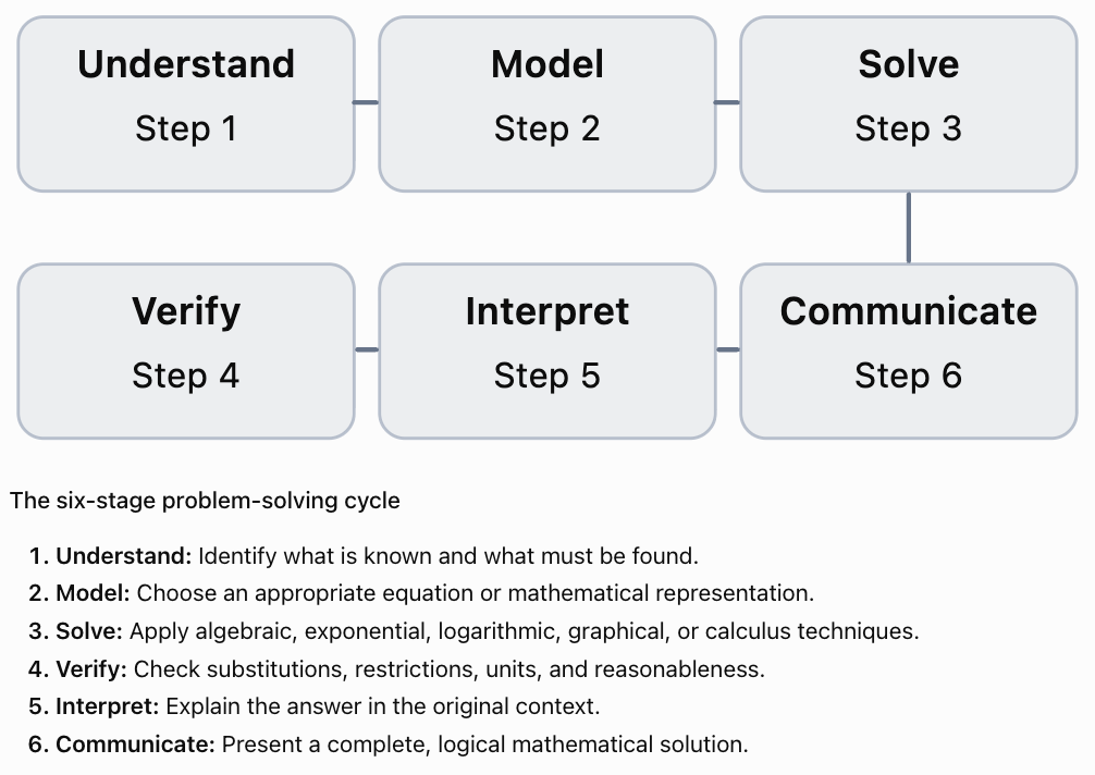
A strong solution should demonstrate all six stages, even when some are completed mentally.

Essential Mathematical Relationships

The following formulas connect many of the topics studied throughout the course.

For logarithmic laws, the arguments M and N must be positive, and the base a must be positive and not equal to 1.

Selecting an Efficient Mathematical Strategy

The structure of a problem often suggests the most efficient approach.

Choosing a strategy before calculating can prevent unnecessary algebra and reduce errors.

Solving Advanced Exponential Equations

Worked Example 1: Equations with a Common Base

Solve:

3^(2x − 1) = 81^(x − 2)

Step 1: Express both sides using base 3.

Since 81 = 3⁴:

3^(2x − 1) = 3^[4(x − 2)]

Step 2: Equate the exponents.

2x − 1 = 4x − 8

Step 3: Solve.

7 = 2x

x = 3.5

Step 4: Verify.

Left side:

3^(2 × 3.5 − 1) = 3⁶ = 729

Right side:

81^(3.5 − 2) = 81¹·⁵ = 729

Both sides agree.

Worked Example 2: Exponential Equations Requiring Substitution

Solve:

4ˣ − 5(2ˣ) + 4 = 0

Notice that:

4ˣ = (2ˣ)²

Step 1: Substitute.

Let:

u = 2ˣ

Then:

u² − 5u + 4 = 0

Step 2: Factorise.

(u − 1)(u − 4) = 0

Therefore:

u = 1 or u = 4

Step 3: Substitute back.

If 2ˣ = 1:

x = 0

If 2ˣ = 4:

x = 2

Solutions: x = 0 or x = 2

This substitution transforms an exponential equation into a familiar quadratic equation.

Worked Example 3: Different Exponential Bases

Solve:

5^(x + 1) = 3^(2x)

Step 1: Take natural logarithms.

ln[5^(x + 1)] = ln[3^(2x)]

Step 2: Apply the power law.

(x + 1)ln(5) = 2x ln(3)

Step 3: Expand.

x ln(5) + ln(5) = 2x ln(3)

Step 4: Collect terms.

ln(5) = x[2ln(3) − ln(5)]

Step 5: Solve.

x = ln(5)/[2ln(3) − ln(5)]

Using:

ln(5) ≈ 1.609438

ln(3) ≈ 1.098612

x ≈ 1.609438/(2.197225 − 1.609438)

x ≈ 2.738

The logarithmic method is efficient because the two exponential expressions cannot easily be rewritten using a common base.

Solving Advanced Logarithmic Equations

Logarithmic equations require particular care because the arguments of logarithms must be positive.

Worked Example 4: Combining Logarithms

Solve:

log₂(x − 1) + log₂(x − 3) = 3

Step 1: Identify domain restrictions.

x − 1 > 0

x − 3 > 0

Therefore:

x > 3

Step 2: Apply the product law.

log₂[(x − 1)(x − 3)] = 3

Step 3: Convert to exponential form.

(x − 1)(x − 3) = 2³

(x − 1)(x − 3) = 8

Step 4: Expand.

x² − 4x + 3 = 8

x² − 4x − 5 = 0

Step 5: Factorise.

(x − 5)(x + 1) = 0

Therefore:

x = 5 or x = −1

Step 6: Check the domain.

Only x = 5 satisfies x > 3.

Final answer: x = 5

The solution x = −1 is extraneous because it makes the logarithmic arguments invalid.

Worked Example 5: Logarithms with Different Bases

Solve:

log₂(x) + log₄(x) = 6

Step 1: Express the logarithms using a common base.

Since 4 = 2²:

log₄(x) = log₂(x)/2

Step 2: Substitute.

log₂(x) + (1/2)log₂(x) = 6

Step 3: Combine like terms.

(3/2)log₂(x) = 6

log₂(x) = 4

Step 4: Convert to exponential form.

x = 2⁴

x = 16

Check:

log₂(16) = 4

log₄(16) = 2

4 + 2 = 6

The solution is correct.

Exponential and Logarithmic Inequalities

Inequalities require attention to the direction of the inequality sign.

For an exponential function with base greater than 1, the function is increasing.

For a base between 0 and 1, the function is decreasing.

Worked Example 6: Exponential Inequality

Solve:

2^(3x − 1) > 16

Rewrite:

16 = 2⁴

Therefore:

2^(3x − 1) > 2⁴

Because base 2 is greater than 1:

3x − 1 > 4

3x > 5

x > 5/3

Worked Example 7: Decreasing Exponential Function

Solve:

(1/3)^(2x + 1) ≤ 1/27

Rewrite:

1/27 = (1/3)³

Therefore:

(1/3)^(2x + 1) ≤ (1/3)³

Since 0 < 1/3 < 1, the exponential function is decreasing.

The inequality reverses when comparing exponents:

2x + 1 ≥ 3

2x ≥ 2

x ≥ 1

Worked Example 8: Logarithmic Inequality

Solve:

ln(x − 2) ≥ 1

Step 1: Identify the domain.

x − 2 > 0

x > 2

Step 2: Convert to exponential form.

Because ln(x) is increasing:

x − 2 ≥ e¹

Step 3: Solve.

x ≥ 2 + e

Approximately:

x ≥ 4.718

This satisfies the original domain restriction.

Comparing Exponential Models

Some problems require us to compare two exponential functions and determine when one becomes greater than the other.

Worked Example 9: Comparing Two Technologies

Two hypothetical computing systems have processing capacities:

A(t) = 800(1.15)ᵗ

B(t) = 500(1.25)ᵗ

where t is measured in years.

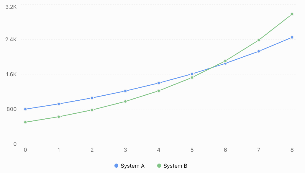
Determine when System B overtakes System A.

Step 1: Set the models equal.

800(1.15)ᵗ = 500(1.25)ᵗ

Step 2: Divide by 500(1.15)ᵗ.

800/500 = (1.25/1.15)ᵗ

1.6 = (25/23)ᵗ

Step 3: Take logarithms.

ln(1.6) = t ln(25/23)

Step 4: Solve.

t = ln(1.6)/ln(25/23)

t ≈ 5.64 years

System B overtakes System A after approximately 5.64 years.

Interpretation

System A begins with greater capacity.

System B has a higher growth rate.

Although System B initially has a disadvantage, its faster exponential growth eventually allows it to overtake System A.

This is a common feature of competing exponential models.

Building Exponential Models from Data

Real-world problems often provide measurements rather than equations.

We must construct the mathematical model before solving the problem.

Worked Example 10: Determining an Exponential Model

A bacterial population is measured at two times.

Assume continuous exponential growth.

Find the growth model and predict the population after 10 hours.

Step 1: Choose the model.

P(t) = P₀eʳᵗ

Since P₀ = 400:

P(t) = 400eʳᵗ

Step 2: Use the second measurement.

1200 = 400e⁶ʳ

Divide by 400:

3 = e⁶ʳ

Step 3: Take natural logarithms.

ln(3) = 6r

r = ln(3)/6

r ≈ 0.1831 h⁻¹

Step 4: Write the model.

P(t) = 400e^[(ln(3)/6)t]

Equivalently:

P(t) = 400 × 3^(t/6)

Step 5: Predict the population after 10 hours.

P(10) = 400 × 3^(10/6)

P(10) ≈ 2,498 bacteria

Evaluating the model

The model assumes that the relative growth rate remains constant.

It may be appropriate over a short period when nutrients and space are plentiful.

Over longer periods, environmental limitations may reduce the growth rate.

A logistic model may eventually become more appropriate.

Multi-Step Financial Applications

Financial problems often combine exponential growth, logarithms, percentages, and comparison of alternative models.

Worked Example 11: Comparing Investment Strategies

An investor has $10,000 and is considering two accounts.

Account A: 5.5% annual interest compounded annually.

Account B: 5.4% nominal annual interest compounded monthly.

Determine which account produces the larger balance after 15 years.

Step 1: Calculate Account A.

A(t) = 10000(1.055)ᵗ

After 15 years:

A(15) = 10000(1.055)¹⁵

A(15) ≈ $22,324.77

Step 2: Calculate Account B.

B(t) = 10000(1 + 0.054/12)^(12t)

After 15 years:

B(15) = 10000(1.0045)¹⁸⁰

B(15) ≈ $22,440.85

Step 3: Compare.

Difference:

22440.85 − 22324.77

Difference ≈ $116.08

Account B produces approximately $116 more under the stated assumptions.

Justifying the result

Although Account B has a lower nominal annual interest rate, monthly compounding produces a higher effective annual rate.

Account A:

EAR = 5.5%

Account B:

EAR = (1.0045)¹² − 1

EAR ≈ 5.536%

Therefore, Account B produces slightly greater growth.

This comparison assumes constant rates and excludes fees, taxes, and other account conditions.

Multi-Step Scientific Applications

Worked Example 12: Radioactive Decay and Half-Life

A radioactive sample initially contains 600 g of a particular isotope.

After 12 years, 150 g of the isotope remains.

Assume exponential decay.

Determine:

a) The decay constant.

b) The half-life.

c) The amount remaining after 20 years.

d) The time required for the amount to fall below 50 g.

Part A: Find the decay constant

Use:

M(t) = M₀e⁻λᵗ

Substitute:

150 = 600e⁻¹²λ

Divide by 600:

0.25 = e⁻¹²λ

Take natural logarithms:

ln(0.25) = −12λ

Therefore:

λ = −ln(0.25)/12

λ ≈ 0.11552 year⁻¹

Part B: Find the half-life

t½ = ln(2)/λ

Substitute:

t½ = 0.693147/0.11552

t½ = 6 years

Part C: Calculate the amount after 20 years

Use the exact half-life form:

M(t) = 600(1/2)^(t/6)

At t = 20:

M(20) = 600(1/2)^(20/6)

M(20) ≈ 59.53 g

Part D: Find when the amount falls below 50 g

Set:

600(1/2)^(t/6) < 50

Divide by 600:

(1/2)^(t/6) < 1/12

Take natural logarithms:

(t/6)ln(1/2) < ln(1/12)

Since ln(1/2) is negative, the inequality reverses when dividing:

t/6 > ln(1/12)/ln(1/2)

Therefore:

t > 6ln(12)/ln(2)

t > 21.51 years

The expected remaining mass falls below 50 g after approximately 21.51 years.

Multi-Step Logarithmic Applications

Worked Example 13: Comparing Chemical Concentrations

Two dilute aqueous solutions have hydrogen ion concentrations:

Solution A: 2.5 × 10⁻³ mol/L

Solution B: 4.0 × 10⁻⁶ mol/L

Calculate:

a) The approximate pH of each solution.

b) The difference in pH.

c) The ratio of their hydrogen ion concentrations.

For sufficiently dilute solutions, use:

pH ≈ −log₁₀([H⁺])

Part A: Calculate the pH values

Solution A:

pH ≈ −log₁₀(2.5 × 10⁻³)

pH ≈ 2.602

Solution B:

pH ≈ −log₁₀(4.0 × 10⁻⁶)

pH ≈ 5.398

Part B: Calculate the pH difference

Difference:

5.398 − 2.602

Difference ≈ 2.796 pH units

Part C: Calculate the concentration ratio

Ratio:

(2.5 × 10⁻³)/(4.0 × 10⁻⁶)

= 625

Solution A has 625 times the hydrogen ion concentration of Solution B.

This is consistent with the logarithmic pH difference because:

10²·⁷⁹⁶ ≈ 625

The calculation illustrates how logarithmic differences correspond to multiplicative ratios.

Combining Exponential Models with Calculus

Calculus allows us to investigate not only how much a quantity changes, but also how quickly it changes.

Worked Example 14: Population Growth and Instantaneous Rate

A population follows:

P(t) = 800e⁰·¹⁵ᵗ

where t is measured in years.

Determine:

a) The population after eight years.

b) The instantaneous growth rate after eight years.

c) The time required for the population to reach 4,000.

Part A: Calculate the population

P(8) = 800e¹·²

Since e¹·² ≈ 3.320117:

P(8) ≈ 800 × 3.320117

P(8) ≈ 2,656 organisms

Part B: Differentiate

P′(t) = 800(0.15)e⁰·¹⁵ᵗ

P′(t) = 120e⁰·¹⁵ᵗ

At t = 8:

P′(8) = 120e¹·²

P′(8) ≈ 398.41 organisms per year

Part C: Solve for time

Set:

4000 = 800e⁰·¹⁵ᵗ

Divide by 800:

5 = e⁰·¹⁵ᵗ

Take natural logarithms:

ln(5) = 0.15t

t = ln(5)/0.15

t ≈ 10.73 years

Interpretation

After eight years, the population is approximately 2,656.

At that instant, the population is increasing at approximately 398 organisms per year.

The population reaches 4,000 after approximately 10.73 years.

This problem combines exponential modelling, differentiation, logarithmic equations, and interpretation of rates.

Logistic Models and Advanced Problem Solving

Exponential growth may be inappropriate when a quantity approaches a limiting value.

A logistic model has the form:

P(t) = K/(1 + Ae⁻ʳᵗ)

where K represents carrying capacity.

Worked Example 15: Logistic Population Growth

A population follows:

P(t) = 10000/(1 + 19e⁻⁰·⁴ᵗ)

where t is measured in years.

Determine:

a) The initial population.

b) The carrying capacity.

c) The population after five years.

d) The time required to reach 8,000.

Part A: Initial population

At t = 0:

P(0) = 10000/(1 + 19)

P(0) = 10000/20

Initial population = 500

Part B: Carrying capacity

The carrying capacity is the limiting value:

K = 10,000

Part C: Population after five years

P(5) = 10000/(1 + 19e⁻²)

Since e⁻² ≈ 0.135335:

P(5) ≈ 10000/[1 + 19(0.135335)]

P(5) ≈ 10000/3.57137

P(5) ≈ 2,800 organisms

Part D: Time required to reach 8,000

Set:

8000 = 10000/(1 + 19e⁻⁰·⁴ᵗ)

Rearrange:

1 + 19e⁻⁰·⁴ᵗ = 10000/8000

1 + 19e⁻⁰·⁴ᵗ = 1.25

Subtract 1:

19e⁻⁰·⁴ᵗ = 0.25

Divide by 19:

e⁻⁰·⁴ᵗ = 1/76

Take natural logarithms:

−0.4t = ln(1/76)

Therefore:

t = ln(76)/0.4

t ≈ 10.83 years

The population reaches 8,000 after approximately 10.83 years.

Comparing exponential and logistic models

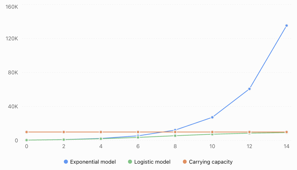
The exponential model continues increasing without bound.

The logistic model approaches a carrying capacity of 10,000.

Choosing between these models requires scientific understanding of the system.

Error Analysis and Verification

A mathematically correct calculation can still produce an inappropriate answer if the model is unsuitable or the assumptions are unrealistic.

Consider the following statement:

"A population doubles every year, so it will continue doubling forever."

The mathematical model might be:

P(t) = P₀2ᵗ

However, this model assumes an unlimited supply of resources and a constant proportional growth rate.

For a real biological population, these assumptions may fail.

Methods of verification

Algebraic verification

Substitute proposed solutions into the original equation.

Domain verification

Check that logarithmic arguments are positive.

Graphical verification

Compare calculated solutions with graphs.

Numerical verification

Use a calculator or spreadsheet to evaluate expressions.

Contextual verification

Check whether answers are physically, financially, or scientifically reasonable.

Dimensional verification

Check that units are consistent.

Worked Example 16: Identifying an Extraneous Solution

Solve:

ln(x − 2) + ln(x + 1) = ln(10)

Step 1: Identify the domain.

x − 2 > 0

x + 1 > 0

Therefore:

x > 2

Step 2: Combine logarithms.

ln[(x − 2)(x + 1)] = ln(10)

Step 3: Equate the arguments.

(x − 2)(x + 1) = 10

Expand:

x² − x − 2 = 10

x² − x − 12 = 0

Factorise:

(x − 4)(x + 3) = 0

Therefore:

x = 4 or x = −3

Step 4: Apply the domain restriction.

Only x = 4 satisfies x > 2.

Final answer: x = 4

The solution x = −3 must be rejected.

Communicating Mathematical Reasoning

A complete mathematical solution should be clear enough for another person to follow and verify.

Good mathematical communication includes:

• Defining variables.

• Stating relevant formulas.

• Showing substitutions.

• Explaining important algebraic steps.

• Identifying domain restrictions.

• Using appropriate units.

• Rounding sensibly.

• Interpreting results in context.

• Justifying the selected model.

Example of weak communication

"Answer = 12.4."

This does not explain what was calculated or why the result is reasonable.

Example of strong communication

"Using the exponential decay model and the measured decay constant, the time required for the sample to decrease to the specified mass is approximately 12.4 years. The result is consistent with the decreasing exponential model because the target mass is smaller than the initial mass."

The second response connects the mathematical calculation to the original situation.

Common Mistakes

Mistake 1: Selecting a formula before understanding the problem

Correction: Identify the quantities, relationships, and unknowns first.

Mistake 2: Confusing exponential and linear growth

Correction: Examine whether the change is additive or multiplicative.

Mistake 3: Applying logarithmic laws incorrectly

For example:

log(a + b) is not generally equal to log(a) + log(b).

Correction: Use logarithmic laws only for valid products, quotients, and powers.

Mistake 4: Ignoring logarithmic domain restrictions

Correction: Require every real logarithmic argument to be positive.

Mistake 5: Forgetting to reverse inequalities

Correction: Remember that logarithmic and exponential functions with bases between 0 and 1 are decreasing.

Mistake 6: Confusing growth factors and growth rates

Correction: Convert percentage rates into multipliers correctly.

Mistake 7: Mixing time units

Correction: Use consistent units for rates and time.

Mistake 8: Rounding too early

Correction: Retain sufficient precision until the final answer.

Mistake 9: Failing to verify solutions

Correction: Substitute results into the original equation and check restrictions.

Mistake 10: Extrapolating models beyond their useful range

Correction: Evaluate assumptions and recognise model limitations.

Mistake 11: Confusing the quantity with its rate of change

Correction: Distinguish between a function and its derivative.

Mistake 12: Giving an answer without interpretation

Correction: Explain what the result means in the original context.

Key Terms

• Exponential Function: Function in which the variable appears in the exponent.

• Logarithmic Function: Inverse of an exponential function.

• Natural Logarithm: Logarithm with base e.

• Growth Factor: Multiplication factor for each time interval.

• Growth Constant: Parameter describing proportional exponential growth.

• Decay Constant: Parameter describing exponential decay.

• Half-Life: Time required for an exponentially decaying quantity to decrease by half.

• Doubling Time: Time required for an exponentially growing quantity to double.

• Compound Interest: Interest calculated on principal and previously accumulated interest.

• Continuous Compounding: Limiting form of increasingly frequent compounding.

• Logistic Growth: Growth that approaches a limiting value.

• Carrying Capacity: Maximum population supported under the assumptions of a logistic model.

• Derivative: Instantaneous rate of change.

• Integral: Mathematical expression associated with accumulation.

• Domain Restriction: Condition limiting allowable input values.

• Extraneous Solution: Apparent solution that does not satisfy the original equation.

• Substitution: Replacing an expression with a new variable to simplify a problem.

• Mathematical Model: Mathematical representation of a real-world process.

• Residual: Difference between an observed and predicted value.

• Extrapolation: Prediction beyond the observed data.

• Verification: Process of checking mathematical results.

• Mathematical Justification: Logical explanation supporting a mathematical method or conclusion.

• Mathematical Communication: Clear presentation of mathematical reasoning and results.

Key Takeaways

• Complex exponential and logarithmic problems often require several mathematical techniques.

• A systematic approach helps organise multi-step reasoning.

• Common bases, substitutions, and logarithms are important methods for solving exponential equations.

• Logarithmic equations require domain restrictions and solution checks.

• Logarithms allow unknown times and growth constants to be calculated.

• Exponential models can be constructed from measurements.

• Competing exponential models can be compared by solving for their intersections.

• Exponential and logistic models describe different long-term behaviours.

• Calculus allows instantaneous rates and accumulated changes to be analysed.

• Mathematical answers must be interpreted within the original context.

• Verification and evaluation of assumptions are essential parts of problem solving.

• Clear communication demonstrates understanding and makes mathematical solutions reliable.

Check Your Understanding

These problems combine concepts from throughout the course. Several require multiple steps and careful interpretation.

Questions

Question 1: Exponential Equation

Solve:

3^(2x) = 27^(x − 1)

Question 2: Exponential Substitution

Solve:

9ˣ − 10(3ˣ) + 9 = 0

Question 3: Different Bases

Solve:

4^(x + 1) = 7ˣ

Question 4: Logarithmic Equation

Solve:

log₃(x − 2) + log₃(x + 2) = 2

Question 5: Logarithmic Inequality

Solve:

ln(2x − 1) > 2

Question 6: Exponential Growth Model

A population increases from 500 to 1,500 over eight years.

Assume continuous exponential growth.

a) Find the growth constant.

b) Write the growth model.

c) Predict the population after 12 years.

Question 7: Comparing Investments

An investor deposits $8,000 into an account earning 6% interest compounded annually.

a) Calculate the balance after 10 years.

b) Determine how long it takes for the balance to double.

Question 8: Radioactive Decay

A radioactive isotope has a half-life of nine years.

A sample initially contains 400 g.

a) Calculate the amount remaining after 27 years.

b) Determine when the amount will fall below 25 g.

Question 9: Comparing Growth Models

Two companies have revenue models:

A(t) = 1000(1.08)ᵗ

B(t) = 700(1.15)ᵗ

Determine when Company B overtakes Company A.

Question 10: Logistic Growth

A population follows:

P(t) = 6000/(1 + 11e⁻⁰·⁵ᵗ)

a) Determine the carrying capacity.

b) Calculate the initial population.

c) Determine when the population reaches 3,000.

Question 11: Chemical Concentration

A dilute aqueous solution has hydrogen ion concentration 5 × 10⁻⁴ mol/L.

Calculate its approximate pH.

Question 12: Exponential Calculus

A population follows:

P(t) = 300e⁰·²ᵗ

a) Find P′(t).

b) Calculate the instantaneous growth rate at t = 5.

c) Calculate the total population increase between t = 0 and t = 5.

Question 13: Evaluating a Model

A company's stored data increases by 35% annually for four years.

Explain two reasons why an exponential model may become unreliable when predicting storage requirements 25 years into the future.

Question 14: Integrated Challenge

A laboratory culture initially contains 800 bacteria.

After four hours, the population reaches 2,400.

Assume continuous exponential growth.

a) Find the growth constant.

b) Calculate the doubling time.

c) Determine when the population reaches 10,000.

d) Calculate the instantaneous growth rate when the population reaches 10,000.

e) Explain one limitation of the model.

Fully Worked Answers

Answer 1: Exponential Equation

3^(2x) = 27^(x − 1)

Since 27 = 3³:

3^(2x) = 3^[3(x − 1)]

Equate exponents:

2x = 3x − 3

x = 3

Answer 2: Exponential Substitution

9ˣ − 10(3ˣ) + 9 = 0

Let:

u = 3ˣ

Then:

u² − 10u + 9 = 0

Factorise:

(u − 1)(u − 9) = 0

Therefore:

u = 1 or u = 9

Substitute back:

3ˣ = 1 gives x = 0.

3ˣ = 9 gives x = 2.

Solutions: x = 0 or x = 2

Answer 3: Different Bases

4^(x + 1) = 7ˣ

Take natural logarithms:

(x + 1)ln(4) = x ln(7)

Expand:

x ln(4) + ln(4) = x ln(7)

Collect terms:

ln(4) = x[ln(7) − ln(4)]

Therefore:

x = ln(4)/[ln(7) − ln(4)]

x ≈ 2.477

Answer 4: Logarithmic Equation

log₃(x − 2) + log₃(x + 2) = 2

Domain:

x > 2

Combine:

log₃[(x − 2)(x + 2)] = 2

Convert to exponential form:

(x − 2)(x + 2) = 9

x² − 4 = 9

x² = 13

x = ±√13

Since x > 2:

x = √13 ≈ 3.606

Answer 5: Logarithmic Inequality

ln(2x − 1) > 2

Domain:

2x − 1 > 0

x > 1/2

Since ln is increasing:

2x − 1 > e²

2x > 1 + e²

x > (1 + e²)/2

Approximately:

x > 4.195

Answer 6: Exponential Growth Model

Initial population = 500

Population after eight years = 1500

Use:

P(t) = 500eʳᵗ

At t = 8:

1500 = 500e⁸ʳ

3 = e⁸ʳ

Take natural logarithms:

ln(3) = 8r

r = ln(3)/8 ≈ 0.13733 year⁻¹

Model:

P(t) = 500e^[(ln(3)/8)t]

After 12 years:

P(12) = 500 × 3^(12/8)

P(12) = 500 × 3¹·⁵

P(12) ≈ 2,598 organisms

Answer 7: Comparing Investments

Initial deposit = $8,000

Annual interest rate = 6%

Part a: Balance after 10 years

A = 8000(1.06)¹⁰

A ≈ $14,326.78

Part b: Doubling time

2 = (1.06)ᵗ

Take natural logarithms:

ln(2) = t ln(1.06)

t = ln(2)/ln(1.06)

t ≈ 11.90 years

With annual interest crediting, the balance first exceeds twice the principal after 12 complete years.

Answer 8: Radioactive Decay

Initial mass = 400 g

Half-life = 9 years

Part a: After 27 years

Number of half-lives:

27/9 = 3

Remaining mass:

M = 400(1/2)³

M = 50 g

Part b: Below 25 g

Set:

400(1/2)^(t/9) < 25

Divide by 400:

(1/2)^(t/9) < 1/16

Since:

1/16 = (1/2)⁴

and the exponential function is decreasing:

t/9 > 4

t > 36 years

The expected remaining mass falls below 25 g after 36 years.

Answer 9: Comparing Growth Models

Set the models equal:

1000(1.08)ᵗ = 700(1.15)ᵗ

Divide:

1000/700 = (1.15/1.08)ᵗ

Take logarithms:

ln(10/7) = t ln(1.15/1.08)

Therefore:

t = ln(10/7)/ln(1.15/1.08)

t ≈ 5.68 years

Company B overtakes Company A after approximately 5.68 years.

Answer 10: Logistic Growth

Given:

P(t) = 6000/(1 + 11e⁻⁰·⁵ᵗ)

Part a: Carrying capacity

K = 6000

Part b: Initial population

P(0) = 6000/(1 + 11)

P(0) = 6000/12

P₀ = 500

Part c: Reaching 3,000

3000 = 6000/(1 + 11e⁻⁰·⁵ᵗ)

Rearrange:

1 + 11e⁻⁰·⁵ᵗ = 2

11e⁻⁰·⁵ᵗ = 1

e⁻⁰·⁵ᵗ = 1/11

Take logarithms:

−0.5t = ln(1/11)

Therefore:

t = ln(11)/0.5

t ≈ 4.80 time units

Answer 11: Chemical Concentration

[H⁺] = 5 × 10⁻⁴ mol/L

Use:

pH ≈ −log₁₀(5 × 10⁻⁴)

pH ≈ −[log₁₀(5) − 4]

pH ≈ −(0.69897 − 4)

pH ≈ 3.301

Answer 12: Exponential Calculus

Given:

P(t) = 300e⁰·²ᵗ

Part a: Differentiate

P′(t) = 300(0.2)e⁰·²ᵗ

P′(t) = 60e⁰·²ᵗ

Part b: Growth rate at t = 5

P′(5) = 60e¹

P′(5) ≈ 60(2.71828)

P′(5) ≈ 163.10 organisms per time unit

Part c: Total population increase

P(5) − P(0) = 300e¹ − 300

= 300(e − 1)

Increase ≈ 515.48 organisms

Answer 13: Evaluating a Model

An exponential model may become unreliable because:

1. The company's growth rate may change as demand, products, or business conditions change.

2. Storage efficiency, compression, retention policies, or technological improvements may alter future storage requirements.

The model may be useful for short-term planning but should be updated regularly rather than extrapolated without review.

Answer 14: Integrated Challenge

Initial population = 800

Population after four hours = 2400

Part a: Growth constant

P(t) = 800eʳᵗ

2400 = 800e⁴ʳ

3 = e⁴ʳ

ln(3) = 4r

r = ln(3)/4 ≈ 0.27465 h⁻¹

Part b: Doubling time

tᵈ = ln(2)/r

tᵈ = 4ln(2)/ln(3)

tᵈ ≈ 2.52 hours

Part c: Reaching 10,000 bacteria

10000 = 800eʳᵗ

12.5 = eʳᵗ

ln(12.5) = rt

t = ln(12.5)/r

t = 4ln(12.5)/ln(3)

t ≈ 9.20 hours

Part d: Instantaneous growth rate

The growth model satisfies:

P′(t) = rP(t)

When P = 10000:

P′ = 0.27465 × 10000

P′ ≈ 2,747 bacteria per hour

Part e: Limitation

The model assumes a constant relative growth rate.

In reality, nutrients, space, oxygen, and waste accumulation may eventually limit bacterial growth.

Therefore, the exponential model may overestimate the population over longer periods.

Final Reflection

Comprehensive problem solving brings together the mathematical ideas developed throughout the exponential and logarithmic functions course.

The most important skill is not memorising individual formulas. It is recognising mathematical structures, selecting suitable strategies, applying techniques accurately, and explaining the meaning of the results.

Exponential and logarithmic functions connect algebra, calculus, financial mathematics, scientific modelling, technological growth, and many other areas of mathematics.

A complete mathematical solution should answer three questions: What is the result? Why is the method mathematically valid? What does the result mean in context?

When these questions are answered clearly, mathematical problem solving becomes a powerful tool for understanding and interpreting the world.