Applications and Connections

4. Connections to Calculus

Introduction

Exponential functions are among the most important functions in mathematics because they connect algebra, functions, rates of change, calculus, differential equations, and mathematical modelling.

In earlier lessons, we explored exponential growth and decay in finance, biology, chemistry, physics, and technology. These applications share a remarkable mathematical property:

The rate at which an exponentially changing quantity changes is proportional to the quantity itself.

This property provides a natural connection to calculus.

For example, a bacterial population may grow more quickly when more bacteria are present. A radioactive sample loses unstable nuclei more rapidly when it contains more undecayed nuclei. Money invested with continuously compounded interest grows at a rate proportional to the current balance.

Calculus allows us to describe these changing rates mathematically.

At the centre of these relationships is the number e, an irrational mathematical constant approximately equal to 2.71828.

The exponential function eˣ is particularly important because its derivative is itself.

This means that the function's instantaneous rate of change is equal to its current value.

In this lesson, we will investigate why e is important, how exponential functions connect to derivatives and integrals, and how these ideas lead to differential equations and advanced mathematical models.

The Number e

The mathematical constant e is approximately:

e ≈ 2.718281828459045...

Like π, e is irrational.

Its decimal representation continues indefinitely without repeating.

The number e appears naturally in:

• Continuous exponential growth and decay.

• Compound interest.

• Differential equations.

• Probability and statistics.

• Calculus.

• Complex numbers.

• Population models.

• Physics and engineering.

Where does e come from?

One way to understand e is through compound interest.

Suppose $1 is invested at a nominal annual interest rate of 100%.

If interest is compounded once per year:

A = (1 + 1)¹ = 2

If compounded twice per year:

A = (1 + 1/2)² = 2.25

If compounded four times per year:

A = (1 + 1/4)⁴ ≈ 2.44141

If compounded increasingly frequently, the value approaches e.

Mathematically:

e = lim(n → ∞) (1 + 1/n)ⁿ

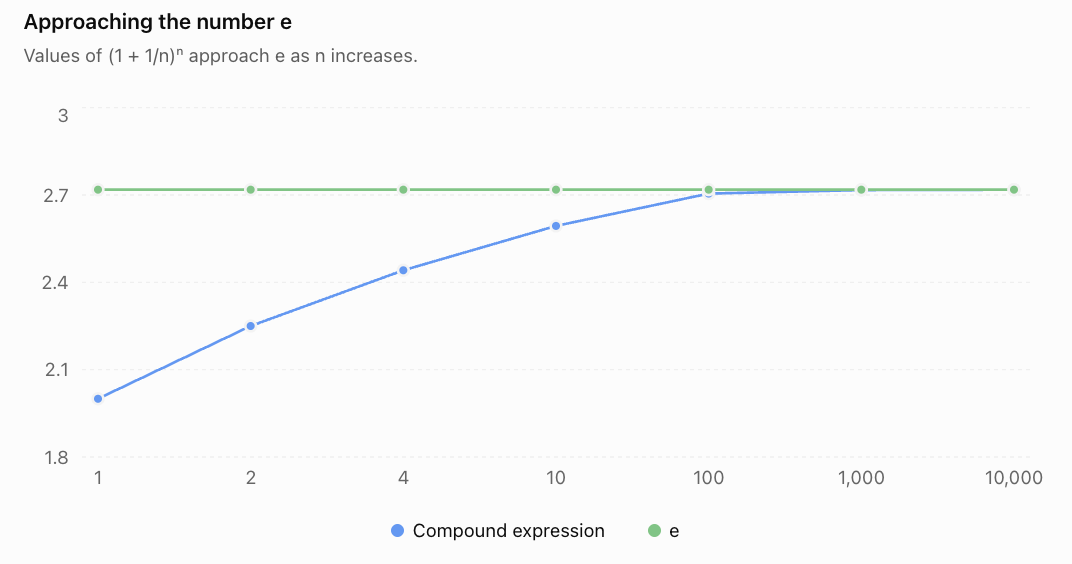
This limit helps explain why e appears in continuously compounded interest.

Natural Exponential Functions

A natural exponential function has the form:

f(x) = eˣ

More generally:

f(x) = Aeᵏˣ

Where:

• A = initial value or scaling constant.

• k = exponential growth or decay constant.

• x = independent variable.

When k > 0, the function represents exponential growth.

When k < 0, it represents exponential decay.

Graph of y = eˣ

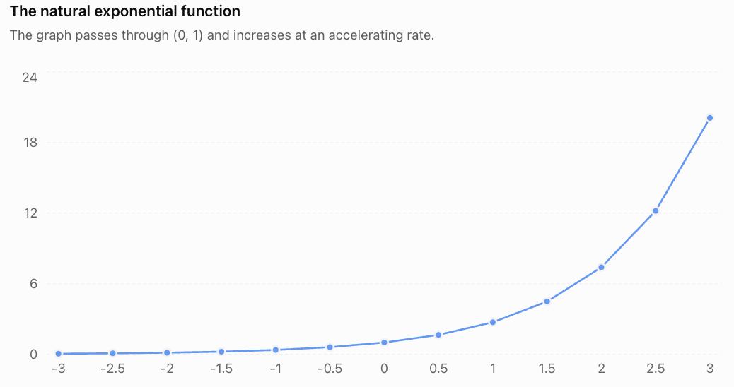
Important properties include:

• Domain: all real numbers.

• Range: y > 0.

• y-intercept: (0, 1).

• Horizontal asymptote: y = 0.

• The function is continuous and differentiable everywhere.

• The function is always increasing.

• Its derivative is equal to the function itself.

The final property makes eˣ especially important in calculus.

Understanding Rates of Change

Calculus is fundamentally concerned with change.

A rate of change describes how quickly one quantity changes in relation to another.

For a function y = f(x), the average rate of change between x = a and x = b is:

Average rate of change = [f(b) − f(a)]/(b − a)

This is the slope of the secant line connecting two points on the graph.

Worked Example 1: Average Rate of Exponential Change

Consider:

f(x) = eˣ

Calculate the average rate of change between x = 0 and x = 2.

Step 1: Evaluate the function.

f(0) = e⁰ = 1

f(2) = e² ≈ 7.3891

Step 2: Apply the formula.

Average rate = (7.3891 − 1)/(2 − 0)

Average rate = 6.3891/2

Average rate ≈ 3.1945

The function increases by an average of approximately 3.1945 units of y per unit of x over this interval.

However, the function does not increase at a constant rate.

Its instantaneous rate of change increases as x increases.

Instantaneous Rate of Change

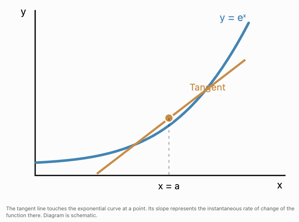
The instantaneous rate of change measures how quickly a function changes at a particular point.

Geometrically, it is the slope of the tangent line at that point.

This is the central idea behind differentiation.

The derivative

The derivative of a function f(x) is written:

f′(x)

or:

dy/dx

The derivative measures the instantaneous rate of change.

It is defined using a limit:

f′(x) = lim(h → 0) [f(x + h) − f(x)]/h

This is called the limit definition of the derivative.

The derivative describes what happens to the average rate of change as the interval becomes arbitrarily small.

Why e Is Special in Differentiation

Consider the exponential function:

f(x) = eˣ

Using the limit definition:

f′(x) = lim(h → 0) [e^(x+h) − eˣ]/h

Use the exponent rule:

e^(x+h) = eˣeʰ

Therefore:

f′(x) = lim(h → 0) [eˣeʰ − eˣ]/h

Factor out eˣ:

f′(x) = eˣ lim(h → 0) [(eʰ − 1)/h]

A fundamental limit is:

lim(h → 0) [(eʰ − 1)/h] = 1

Therefore:

d/dx(eˣ) = eˣ

This is one of the most important results in calculus.

The derivative of eˣ is exactly eˣ.

Interpreting the result

At x = 0:

e⁰ = 1

The slope of the tangent line is also 1.

At x = 1:

e¹ ≈ 2.718

The slope is approximately 2.718.

At x = 2:

e² ≈ 7.389

The slope is approximately 7.389.

As the function increases, its instantaneous rate of increase also increases.

Differentiating General Exponential Functions

For the natural exponential function:

d/dx(eᵏˣ) = keᵏˣ

This follows from the chain rule.

More generally:

d/dx(Aeᵏˣ) = Akeᵏˣ

Where A and k are constants.

Worked Example 2: Differentiating an Exponential Function

Find the derivative of:

f(x) = 5e³ˣ

Use:

d/dx(Aeᵏˣ) = Akeᵏˣ

Substitute:

f′(x) = 5 × 3e³ˣ

f′(x) = 15e³ˣ

Worked Example 3: Exponential Decay

Find the derivative of:

f(t) = 200e⁻⁰·⁴ᵗ

Using the same rule:

f′(t) = 200(−0.4)e⁻⁰·⁴ᵗ

f′(t) = −80e⁻⁰·⁴ᵗ

The derivative is negative, indicating that the quantity decreases over time.

Its magnitude becomes smaller as the quantity approaches zero.

Differentiating Exponential Functions with Other Bases

Not every exponential function uses base e.

Consider:

f(x) = aˣ

where a > 0 and a ≠ 1.

The derivative is:

d/dx(aˣ) = aˣln(a)

For example:

d/dx(2ˣ) = 2ˣln(2)

d/dx(5ˣ) = 5ˣln(5)

d/dx(10ˣ) = 10ˣln(10)

Why does the natural exponential function have such a simple derivative?

Because:

ln(e) = 1

Therefore:

d/dx(eˣ) = eˣln(e) = eˣ

Worked Example 4: Differentiating 2ˣ

Find the derivative of:

f(x) = 2ˣ

Use:

f′(x) = 2ˣln(2)

Since ln(2) ≈ 0.693147:

f′(x) ≈ 0.693147 × 2ˣ

At x = 3:

f′(3) = 2³ln(2)

f′(3) = 8(0.693147)

f′(3) ≈ 5.5452

The instantaneous rate of change at x = 3 is approximately 5.5452.

Interpreting Rates in Exponential Models

Suppose a population follows:

P(t) = P₀eʳᵗ

Differentiate:

P′(t) = rP₀eʳᵗ

Since P(t) = P₀eʳᵗ:

P′(t) = rP(t)

This tells us that the instantaneous population growth rate is proportional to the current population.

Worked Example 5: Population Growth Rate

A bacterial population is modelled by:

P(t) = 500e⁰·²ᵗ

where t is measured in hours.

Calculate the population and its instantaneous growth rate after five hours.

Step 1: Calculate the population.

P(5) = 500e¹

P(5) ≈ 500(2.71828)

P(5) ≈ 1,359 bacteria

Step 2: Differentiate.

P′(t) = 500(0.2)e⁰·²ᵗ

P′(t) = 100e⁰·²ᵗ

Step 3: Evaluate at t = 5.

P′(5) = 100e¹

P′(5) ≈ 272 bacteria per hour

Interpretation

After five hours, the model predicts approximately 1,359 bacteria.

At that instant, the population is increasing at approximately 272 bacteria per hour.

The population and growth rate are different quantities.

The population is measured in bacteria.

The instantaneous growth rate is measured in bacteria per hour.

Exponential Decay and Derivatives

For exponential decay:

N(t) = N₀e⁻λᵗ

where λ > 0.

Differentiate:

N′(t) = −λN₀e⁻λᵗ

Therefore:

N′(t) = −λN(t)

The negative sign indicates that the quantity is decreasing.

The magnitude of the rate of decay is:

|N′(t)| = λN(t)

This means that a larger radioactive sample has a greater expected number of decays per unit time.

Worked Example 6: Radioactive Decay Rate

A radioactive sample follows:

N(t) = 10000e⁻⁰·¹ᵗ

where t is measured in years.

Calculate the expected number of undecayed nuclei and the instantaneous decay rate after 10 years.

Step 1: Calculate the quantity remaining.

N(10) = 10000e⁻¹

N(10) ≈ 10000(0.367879)

N(10) ≈ 3,679 nuclei

Step 2: Differentiate.

N′(t) = −1000e⁻⁰·¹ᵗ

Step 3: Evaluate.

N′(10) = −1000e⁻¹

N′(10) ≈ −367.88 nuclei per year

The negative value indicates a decreasing population of undecayed nuclei.

The expected rate of decay at that time is approximately 368 nuclei per year.

Connecting Exponential Functions to Integration

Differentiation measures instantaneous rates of change.

Integration is closely related to accumulation and total change.

An integral can be used to calculate quantities such as:

• Total population increase over a time interval.

• Accumulated radioactive decays.

• Total energy transferred.

• Total fluid flowing through a system.

• Accumulated interest under suitable models.

The indefinite integral

An indefinite integral represents a family of antiderivatives.

Because:

d/dx(eˣ) = eˣ

we have:

∫eˣ dx = eˣ + C

Where C is the constant of integration.

Why do we need C?

The derivative of eˣ is eˣ.

But the derivative of eˣ + 5 is also eˣ.

Likewise, the derivative of eˣ − 12 is eˣ.

Every constant disappears during differentiation.

Therefore, indefinite integration includes an arbitrary constant.

Integrating General Exponential Functions

For k ≠ 0:

∫eᵏˣ dx = (1/k)eᵏˣ + C

More generally:

∫Aeᵏˣ dx = (A/k)eᵏˣ + C

Worked Example 7: Integrating an Exponential Function

Evaluate:

∫6e²ˣ dx

Use:

∫Aeᵏˣ dx = (A/k)eᵏˣ + C

Therefore:

∫6e²ˣ dx = (6/2)e²ˣ + C

Answer: 3e²ˣ + C

Checking the answer

Differentiate:

d/dx(3e²ˣ) = 3(2)e²ˣ

= 6e²ˣ

This matches the original integrand.

Definite Integrals and Accumulation

A definite integral calculates accumulated change over an interval.

For example:

∫ₐᵇ eˣ dx = eᵇ − eᵃ

This follows from the Fundamental Theorem of Calculus.

Worked Example 8: Evaluating a Definite Integral

Evaluate:

∫₀² eˣ dx

Step 1: Find an antiderivative.

∫eˣ dx = eˣ + C

Step 2: Apply the limits.

∫₀² eˣ dx = e² − e⁰

= e² − 1

Step 3: Evaluate.

≈ 7.389056 − 1

Answer ≈ 6.3891

Visualising the area

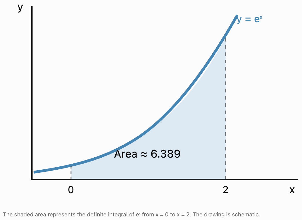
The definite integral represents the area under the curve between the two limits because eˣ is positive.

The Fundamental Theorem of Calculus

The Fundamental Theorem of Calculus connects differentiation and integration.

In simplified terms:

Differentiation and integration are inverse processes, up to an additive constant.

If F′(x) = f(x), then:

∫ₐᵇ f(x) dx = F(b) − F(a)

For exponential functions:

If f(x) = eˣ, then F(x) = eˣ.

Therefore:

∫ₐᵇ eˣ dx = eᵇ − eᵃ

This connection allows us to move between instantaneous rates and accumulated quantities.

Example: Population Change

Suppose:

P′(t) = 100e⁰·²ᵗ

The total population increase from t = 0 to t = 5 is:

∫₀⁵ 100e⁰·²ᵗ dt

Integrate:

= [500e⁰·²ᵗ]₀⁵

= 500e¹ − 500e⁰

= 500(e − 1)

≈ 500(1.71828)

Total population increase ≈ 859 organisms

This matches the difference between the population at t = 5 and the initial population.

Differential Equations and Exponential Functions

A differential equation is an equation involving a function and one or more of its derivatives.

Exponential functions are particularly important because they naturally solve many differential equations.

Consider:

dy/dt = ky

This equation states:

"The instantaneous rate of change of y is proportional to y itself."

Its general solution is:

y(t) = Ceᵏᵗ

where C is a constant determined by an initial condition.

Why does this work?

Suppose:

y(t) = Ceᵏᵗ

Differentiate:

dy/dt = Ckeᵏᵗ

Factor out k:

dy/dt = k(Ceᵏᵗ)

Since y = Ceᵏᵗ:

dy/dt = ky

Therefore, the exponential function satisfies the differential equation.

Worked Example 9: Solving a Differential Equation

A population satisfies:

dP/dt = 0.3P

Initially:

P(0) = 400

Find P(t).

Step 1: Identify the general solution.

P(t) = Ce⁰·³ᵗ

Step 2: Apply the initial condition.

P(0) = Ce⁰

400 = C

Step 3: Write the particular solution.

P(t) = 400e⁰·³ᵗ

Calculate the population after four years

P(4) = 400e¹·²

Since e¹·² ≈ 3.320117:

P(4) ≈ 400 × 3.320117

P(4) ≈ 1,328 organisms

The differential equation describes the rate of growth.

The exponential solution describes the population itself.

Connections to Advanced Mathematics

Exponential functions appear throughout higher mathematics.

1. Differential Equations

Exponential functions solve equations in which rates of change depend on current values.

Applications include population growth, radioactive decay, electrical circuits, and chemical kinetics.

2. Calculus of Several Variables

Exponential functions can depend on more than one variable.

For example:

f(x, t) = Ae⁻ᵏᵗ sin(x)

Such functions appear in mathematical models involving time-dependent waves, diffusion, and other physical processes.

Partial derivatives describe how the function changes with respect to one variable while holding others constant.

3. Complex Numbers

Exponential functions extend naturally to complex numbers.

One of the most famous mathematical identities is Euler's formula:

eⁱᶿ = cos(θ) + i sin(θ)

where i² = −1.

This connects exponential functions, trigonometry, and complex numbers.

For θ = π:

eⁱπ = −1

Therefore:

eⁱπ + 1 = 0

This is known as Euler's identity.

4. Probability and Statistics

The exponential function appears in probability distributions.

For example, the exponential distribution has probability density function:

f(t) = λe⁻λᵗ, for t ≥ 0

where λ > 0.

It can model waiting times between events in certain random processes with constant event rates.

5. Advanced Mathematical Modelling

Exponential functions also appear in:

• Heat transfer.

• Electrical circuit analysis.

• Pharmacokinetics.

• Chemical reaction rates.

• Population dynamics.

• Financial mathematics.

• Signal processing.

• Machine learning.

The importance of exponential functions comes from their ability to connect mathematical structure with changing real-world systems.

Authentic Application: A Cooling System

An electronic component begins at 90°C in a room maintained at 25°C.

Its temperature follows:

T(t) = 25 + 65e⁻⁰·¹ᵗ

where t is measured in minutes.

We want to calculate its temperature, cooling rate, and the time required to reach 40°C.

Part A: Calculate the temperature after 10 minutes

T(10) = 25 + 65e⁻¹

Since e⁻¹ ≈ 0.367879:

T(10) ≈ 25 + 65(0.367879)

T(10) ≈ 25 + 23.9121

T(10) ≈ 48.91°C

Part B: Find the instantaneous cooling rate

Differentiate:

T′(t) = 65(−0.1)e⁻⁰·¹ᵗ

T′(t) = −6.5e⁻⁰·¹ᵗ

At t = 10:

T′(10) = −6.5e⁻¹

T′(10) ≈ −6.5(0.367879)

T′(10) ≈ −2.39°C/min

The component is cooling at approximately 2.39°C per minute after 10 minutes.

Part C: Find when the temperature reaches 40°C

Set:

40 = 25 + 65e⁻⁰·¹ᵗ

Subtract 25:

15 = 65e⁻⁰·¹ᵗ

Divide by 65:

15/65 = e⁻⁰·¹ᵗ

Take natural logarithms:

ln(15/65) = −0.1t

Therefore:

t = ln(15/65)/(−0.1)

t ≈ 14.66 minutes

The model predicts that the component reaches 40°C after approximately 14.66 minutes.

Part D: Interpret the model

The temperature approaches the ambient temperature of 25°C.

The cooling rate is initially relatively large because the temperature difference is large.

As the component cools, the temperature difference decreases, so the magnitude of the cooling rate becomes smaller.

This is a practical example of how exponential functions, differentiation, logarithms, and differential equations work together.

Common Mistakes

Mistake 1: Confusing e with a variable

The symbol e represents a mathematical constant.

Correction: Remember that e ≈ 2.71828.

Mistake 2: Assuming all exponential derivatives are unchanged

The derivative of eˣ is eˣ, but the derivative of e³ˣ is 3e³ˣ.

Correction: Apply the chain rule.

Mistake 3: Forgetting the logarithm when differentiating aˣ

The derivative of aˣ is aˣln(a).

Correction: Remember that the natural exponential function is the special case where a = e.

Mistake 4: Confusing a function with its derivative

The population and its rate of growth are different quantities.

Correction: Check the units of each result.

Mistake 5: Forgetting the negative sign in exponential decay

For e⁻λᵗ, the derivative includes a factor of −λ.

Correction: Differentiate the exponent carefully.

Mistake 6: Forgetting the constant of integration

Indefinite integrals require + C.

Correction: Include the arbitrary constant unless evaluating a definite integral.

Mistake 7: Multiplying instead of dividing during integration

The integral of e³ˣ is (1/3)e³ˣ + C, not 3e³ˣ + C.

Correction: Reverse the chain rule.

Mistake 8: Confusing average and instantaneous rates

Average rate of change is calculated over an interval.

Instantaneous rate of change is calculated at a particular point.

Correction: Use secant slopes for averages and derivatives for instantaneous rates.

Mistake 9: Ignoring units

A derivative represents a rate, so its units differ from those of the original quantity.

Correction: State units clearly.

Mistake 10: Treating a mathematical model as exact reality

Exponential models depend on assumptions.

Correction: Evaluate whether the underlying process is appropriately represented.

Key Terms

• Calculus: Branch of mathematics concerned with change and accumulation.

• e: Irrational mathematical constant approximately equal to 2.71828.

• Natural Exponential Function: Exponential function with base e.

• Limit: Value approached by a function or sequence.

• Rate of Change: Measure of how one quantity changes relative to another.

• Average Rate of Change: Change in a function divided by change in its independent variable over an interval.

• Instantaneous Rate of Change: Rate of change at a particular point.

• Derivative: Mathematical expression describing instantaneous rate of change.

• Differentiation: Process of finding derivatives.

• Tangent Line: Line whose slope represents the instantaneous rate of change at a point on a differentiable curve.

• Secant Line: Line passing through two points on a curve.

• Chain Rule: Rule for differentiating composite functions.

• Integral: Mathematical expression related to accumulation and antiderivatives.

• Indefinite Integral: Family of antiderivatives.

• Definite Integral: Integral evaluated over a specified interval.

• Antiderivative: Function whose derivative is a given function.

• Constant of Integration: Arbitrary constant added to an indefinite integral.

• Fundamental Theorem of Calculus: Theorem connecting differentiation and integration.

• Differential Equation: Equation involving a function and its derivatives.

• Initial Condition: Specified value used to determine a particular solution.

• Exponential Growth Constant: Parameter describing proportional exponential growth.

• Decay Constant: Positive parameter describing exponential decay.

• Euler's Formula: Identity connecting complex exponentials with trigonometric functions.

• Euler's Identity: Special case eⁱπ + 1 = 0.

• Mathematical Model: Mathematical representation of a real-world process.

Key Takeaways

• The number e arises naturally in continuous growth and compounding.

• The natural exponential function eˣ has the special property that its derivative equals itself.

• Derivatives measure instantaneous rates of change.

• Exponential growth models have rates proportional to their current values.

• Exponential decay models have negative derivatives.

• The derivative of Aeᵏˣ is Akeᵏˣ.

• The derivative of aˣ is aˣln(a).

• Integration reverses differentiation, up to an additive constant.

• The integral of eᵏˣ is (1/k)eᵏˣ + C for k ≠ 0.

• Definite integrals can calculate accumulated change.

• Exponential functions solve differential equations of the form dy/dt = ky.

• Exponential functions connect calculus with complex numbers, probability, physics, biology, and engineering.

• Understanding exponential functions provides a foundation for advanced mathematical modelling.

Check Your Understanding

Questions

Question 1: The Number e

Explain why e appears naturally in continuously compounded interest.

Question 2: Natural Exponential Functions

State the value of e⁰ and explain its importance for the graph of y = eˣ.

Question 3: Average Rate of Change

Calculate the average rate of change of f(x) = eˣ between x = 0 and x = 1.

Question 4: Differentiation

Differentiate:

f(x) = eˣ

Question 5: Chain Rule

Differentiate:

f(x) = 4e²ˣ

Question 6: Exponential Decay

Differentiate:

N(t) = 500e⁻⁰·³ᵗ

Question 7: Other Exponential Bases

Differentiate:

f(x) = 3ˣ

Question 8: Population Growth Rate

A population follows:

P(t) = 200e⁰·⁴ᵗ

Calculate the instantaneous growth rate at t = 3.

Question 9: Indefinite Integration

Evaluate:

∫5eˣ dx

Question 10: Integration with the Chain Rule

Evaluate:

∫8e⁴ˣ dx

Question 11: Definite Integration

Evaluate:

∫₀¹ e²ˣ dx

Question 12: Differential Equations

Solve:

dy/dt = 0.2y

given:

y(0) = 300

Question 13: Cooling Model

An object follows:

T(t) = 20 + 50e⁻⁰·²ᵗ

Calculate its instantaneous cooling rate at t = 5.

Question 14: Conceptual Understanding

Explain why the derivative of eˣ is especially important in calculus.

Question 15: Connecting Calculus and Modelling

A population grows according to:

P(t) = 1000e⁰·¹ᵗ

Calculate:

a) The population after 10 years.

b) The instantaneous growth rate after 10 years.

c) The total population increase over the first 10 years.

Fully Worked Answers

Answer 1: The Number e

The number e appears when interest is compounded increasingly frequently.

The expression:

(1 + 1/n)ⁿ

approaches e as n approaches infinity.

This leads to the continuous compounding formula:

A = Peʳᵗ

Answer 2: Natural Exponential Functions

e⁰ = 1

Therefore:

f(0) = 1

The graph of y = eˣ passes through:

(0, 1)

Answer 3: Average Rate of Change

Average rate:

[f(1) − f(0)]/(1 − 0)

= (e − 1)/1

= e − 1

Average rate ≈ 1.7183

Answer 4: Differentiation

Given:

f(x) = eˣ

The derivative is:

f′(x) = eˣ

Answer 5: Chain Rule

Given:

f(x) = 4e²ˣ

Differentiate:

f′(x) = 4(2)e²ˣ

f′(x) = 8e²ˣ

Answer 6: Exponential Decay

Given:

N(t) = 500e⁻⁰·³ᵗ

Differentiate:

N′(t) = 500(−0.3)e⁻⁰·³ᵗ

N′(t) = −150e⁻⁰·³ᵗ

Answer 7: Other Exponential Bases

Given:

f(x) = 3ˣ

Use:

d/dx(aˣ) = aˣln(a)

Therefore:

f′(x) = 3ˣln(3)

Answer 8: Population Growth Rate

Given:

P(t) = 200e⁰·⁴ᵗ

Differentiate:

P′(t) = 80e⁰·⁴ᵗ

At t = 3:

P′(3) = 80e¹·²

Since e¹·² ≈ 3.320117:

P′(3) ≈ 80(3.320117)

P′(3) ≈ 265.61 organisms per time unit

Answer 9: Indefinite Integration

Evaluate:

∫5eˣ dx

Since the antiderivative of eˣ is eˣ:

Answer: 5eˣ + C

Answer 10: Integration with the Chain Rule

Evaluate:

∫8e⁴ˣ dx

Use:

∫Aeᵏˣ dx = (A/k)eᵏˣ + C

Therefore:

∫8e⁴ˣ dx = (8/4)e⁴ˣ + C

Answer: 2e⁴ˣ + C

Answer 11: Definite Integration

Evaluate:

∫₀¹ e²ˣ dx

Antiderivative:

(1/2)e²ˣ

Apply the limits:

= (1/2)e² − (1/2)e⁰

= (e² − 1)/2

Since e² ≈ 7.389056:

= (7.389056 − 1)/2

Answer ≈ 3.1945

Answer 12: Differential Equations

Given:

dy/dt = 0.2y

General solution:

y(t) = Ce⁰·²ᵗ

Apply the initial condition:

y(0) = 300

300 = Ce⁰

C = 300

Answer: y(t) = 300e⁰·²ᵗ

Answer 13: Cooling Model

Given:

T(t) = 20 + 50e⁻⁰·²ᵗ

Differentiate:

T′(t) = −10e⁻⁰·²ᵗ

At t = 5:

T′(5) = −10e⁻¹

T′(5) ≈ −10(0.367879)

T′(5) ≈ −3.68°C per time unit

The negative sign indicates that the object is cooling.

Answer 14: Conceptual Understanding

The derivative of eˣ is equal to eˣ.

This means that the instantaneous rate of change of the function is equal to its current value.

This property makes exponential functions natural solutions to differential equations involving proportional growth and decay.

It also simplifies differentiation, integration, and advanced mathematical modelling.

Answer 15: Connecting Calculus and Modelling

Given:

P(t) = 1000e⁰·¹ᵗ

Part a: Population after 10 years

P(10) = 1000e¹

P(10) ≈ 1000(2.71828)

P(10) ≈ 2,718 organisms

Part b: Instantaneous growth rate

Differentiate:

P′(t) = 100e⁰·¹ᵗ

At t = 10:

P′(10) = 100e¹

P′(10) ≈ 271.83 organisms per year

Part c: Total population increase

Initial population:

P(0) = 1000

Population after 10 years:

P(10) ≈ 2718.28

Total increase:

2718.28 − 1000

Total increase ≈ 1,718 organisms

We can also calculate this using integration:

∫₀¹⁰ P′(t) dt = ∫₀¹⁰ 100e⁰·¹ᵗ dt

= [1000e⁰·¹ᵗ]₀¹⁰

= 1000e − 1000

≈ 1718.28

Both methods produce the same result.

Final Reflection

Exponential functions provide one of the most important connections between algebra and calculus.

The number e is especially significant because the natural exponential function has the remarkable property that its derivative is equal to itself.

This allows exponential functions to describe processes in which the instantaneous rate of change is proportional to the current quantity.

Differentiation helps us calculate rates of growth and decay, while integration allows us to calculate accumulated changes. Differential equations bring these ideas together to describe how real systems evolve.

These relationships extend far beyond introductory calculus into physics, chemistry, biology, engineering, finance, probability, and advanced mathematics.

Understanding exponential functions is therefore more than learning a particular family of equations. It is developing a mathematical language for describing change, accumulation, and the relationships between quantities and their rates of change.