Applications and Connections
3. Exponential Models in Technology
Learning outcomes
- I can explain exponential growth in computing.
- I can analyse information growth.
- I can recognise exponential trends in technology.
- I can interpret technological data.
- I can solve technology-based applications.
Introduction
Technology develops through processes that can produce rapid and sometimes surprising changes. Computing power, data storage, network activity, digital information, and the number of connected devices have all experienced periods of substantial growth.
One of the most important mathematical tools for understanding these changes is the exponential function.
Consider a computer system whose processing capacity doubles every two years. Initially, the increase may appear modest. However, repeated doubling produces increasingly large changes.
A system with an initial capacity of 100 units would develop as follows:
|
Time (years) |
Processing capacity |
|---|---|
|
0 |
100 |
|
2 |
200 |
|
4 |
400 |
|
6 |
800 |
|
8 |
1,600 |
|
10 |
3,200 |
After ten years, the capacity has increased by a factor of 32.
This is not linear growth. The capacity does not increase by the same amount every two years. Instead, it multiplies by the same factor.
Exponential models help us investigate technological growth, estimate future requirements, compare development trends, and understand why seemingly small percentage changes can produce enormous long-term effects.
However, exponential growth cannot continue indefinitely in every technological system. Physical limitations, economic constraints, market saturation, and changes in technology can alter growth patterns.
In this lesson, we will explore exponential growth in computing, digital information, data storage, network systems, and other technological applications. We will also learn to interpret technological data critically and evaluate the limitations of exponential models.
Understanding Exponential Growth
An exponential relationship occurs when a quantity changes by a constant percentage or multiplication factor over equal intervals.
The general discrete exponential model is:
Q(t) = Q₀bᵗ
Where:
-
Q(t) = quantity after time t.
-
Q₀ = initial quantity.
-
b = multiplication factor per time unit.
-
t = elapsed time.
If b > 1, the model represents exponential growth.
If 0 < b < 1, the model represents exponential decay.
For continuous exponential growth, we use:
Q(t) = Q₀eᵏᵗ
Where:
-
e ≈ 2.71828.
-
k = continuous growth constant.
Comparing linear and exponential growth
Suppose two computer systems begin with a processing capacity of 100 units.
System A increases by 100 units every two years.
System B doubles every two years.
|
Time (years) |
Linear model |
Exponential model |
|---|---|---|
|
0 |
100 |
100 |
|
2 |
200 |
200 |
|
4 |
300 |
400 |
|
6 |
400 |
800 |
|
8 |
500 |
1,600 |
|
10 |
600 |
3,200 |
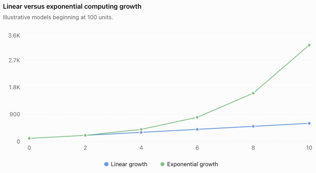
The linear model increases at a constant absolute rate.
The exponential model increases at a constant proportional rate.
This difference becomes especially important over long periods.
Exponential Growth in Computing
Computing technology has experienced periods of rapid improvements in processing capability, memory capacity, and component density.
Exponential models can describe these trends over suitable time intervals.
Moore's Law
One of the best-known historical observations in computing is Moore's law.
Moore's Law describes a historical trend in which the number of transistors on an integrated circuit increased approximately exponentially over time.
The commonly cited later formulation describes transistor counts doubling approximately every two years.
It is important to recognise that Moore's Law is an empirical technological observation, not a physical law guaranteeing future exponential growth.
Transistor density, processing speed, energy efficiency, and computing performance are related but distinct quantities. They do not necessarily increase at the same rate.
A simplified transistor growth model
Suppose a computer chip initially contains 2 million transistors, and the number doubles every two years.
The model is:
N(t) = 2,000,000 × 2^(t/2)
where t is measured in years.
Worked Example 1: Transistor Growth
Estimate the transistor count after eight years.
Step 1: Write the model.
N(t) = 2,000,000 × 2^(t/2)
Step 2: Substitute t = 8.
N(8) = 2,000,000 × 2^(8/2)
N(8) = 2,000,000 × 2⁴
Step 3: Evaluate.
N(8) = 2,000,000 × 16
N(8) = 32,000,000 transistors
The model predicts 32 million transistors after eight years.
Interpreting the result
The model predicts that the transistor count increases by a factor of 16 over eight years.
It does not establish that a chip with 16 times as many transistors is 16 times faster.
Actual performance depends on architecture, memory systems, clock speed, software, power constraints, and many other factors.
Doubling Time
Doubling time is particularly useful when analysing technological growth.
If a quantity doubles every T time units:
Q(t) = Q₀ × 2^(t/T)
Where:
-
Q₀ = initial quantity.
-
T = doubling time.
-
t = elapsed time.
Worked Example 2: Data Storage Capacity
A storage technology has a capacity of 500 GB and follows a hypothetical model in which capacity doubles every three years.
Calculate the capacity after 12 years.
Q(t) = 500 × 2^(t/3)
Substitute:
Q(12) = 500 × 2⁴
Q(12) = 500 × 16
Q(12) = 8,000 GB
Using decimal storage units:
8,000 GB = 8 TB
The predicted capacity after 12 years is 8 TB.
This is a mathematical projection, not a guarantee about future storage products.
Continuous Growth and Doubling Time
For a continuous exponential model:
Q(t) = Q₀eᵏᵗ
The doubling time is:
T = ln(2)/k
Equivalently:
k = ln(2)/T
Worked Example 3: Calculating a Growth Constant
A hypothetical computing capability doubles every 18 months.
Calculate the continuous growth constant in year⁻¹.
Convert the doubling time:
18 months = 1.5 years
Use:
k = ln(2)/1.5
k ≈ 0.693147/1.5
k ≈ 0.4621 year⁻¹
The model can be written as:
Q(t) = Q₀e⁰·⁴⁶²¹ᵗ
where t is measured in years.
The continuous growth constant is not the same as the effective annual percentage increase.
The effective annual growth factor is:
e⁰·⁴⁶²¹ ≈ 1.5874
Therefore, the effective annual increase is approximately:
58.74% per year
Analysing Information Growth
The amount of digital information stored, transmitted, and processed can increase rapidly.
Examples include:
-
Scientific datasets.
-
Digital photographs and videos.
-
Cloud storage.
-
Sensor measurements.
-
Internet traffic.
-
Business transaction records.
-
Machine-learning training data.
Not every form of digital information grows exponentially, and growth rates can change substantially over time.
However, exponential models are useful when data volumes increase by approximately constant percentages over equal periods.
Worked Example 4: Digital Information Growth
A research laboratory stores 12 TB of data.
Its stored data volume increases by 30% per year.
Assume this rate remains constant for five years.
The model is:
D(t) = 12(1.30)ᵗ
Calculate the amount of stored data after five years.
D(5) = 12(1.30)⁵
Since:
(1.30)⁵ = 3.71293
D(5) = 12 × 3.71293
D(5) ≈ 44.56 TB
The laboratory would need approximately 44.56 TB of storage after five years under the model.
Interpreting the result
The initial storage requirement is 12 TB.
After five years, the model predicts approximately 44.56 TB.
The required capacity increases by approximately 32.56 TB.
This illustrates why organisations must plan for future storage requirements rather than considering only their current needs.
Comparing Storage Growth Rates
Suppose two organisations begin with 10 TB of data.
Organisation A experiences 15% annual growth.
Organisation B experiences 30% annual growth.
Their models are:
A(t) = 10(1.15)ᵗ
B(t) = 10(1.30)ᵗ
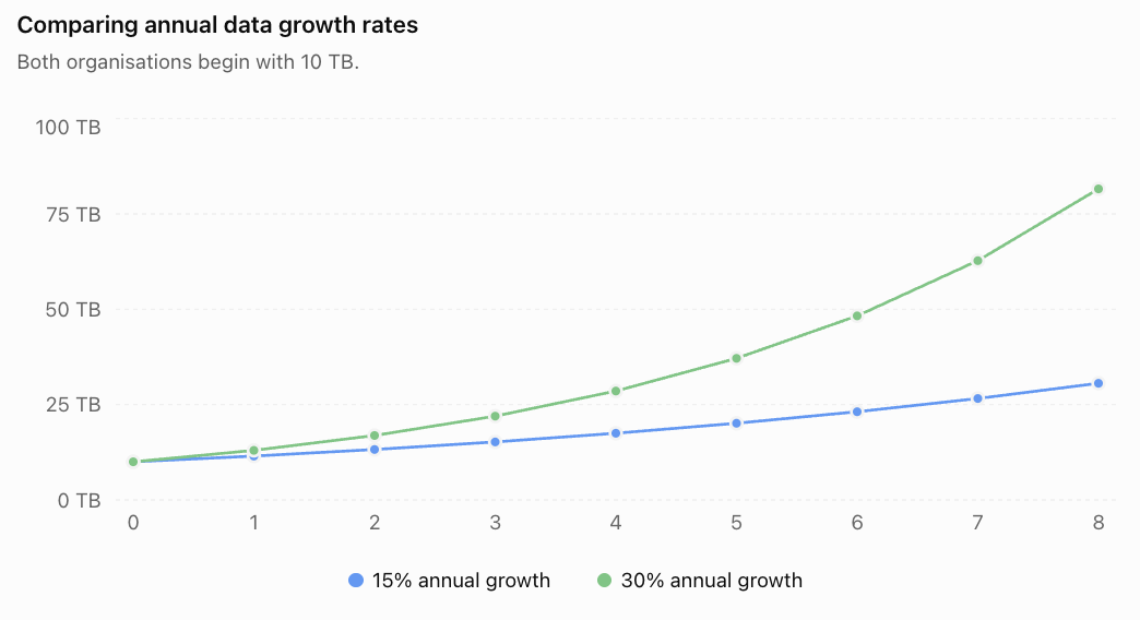
After eight years:
Organisation A requires approximately 30.59 TB.
Organisation B requires approximately 81.57 TB.
Although the growth rates differ by only 15 percentage points, the long-term storage requirements differ substantially.
This is a central feature of exponential growth.
Recognising Exponential Trends in Technological Data
A technological trend should not be described as exponential simply because its graph curves upward.
To identify exponential growth, we should examine the mathematical relationship between successive observations.
Constant differences versus constant ratios
For equally spaced time intervals:
-
Linear growth produces constant first differences.
-
Exponential growth produces constant ratios.
Consider two datasets.
|
Year |
Dataset A |
Dataset B |
|---|---|---|
|
0 |
100 |
100 |
|
1 |
150 |
150 |
|
2 |
200 |
225 |
|
3 |
250 |
337.5 |
|
4 |
300 |
506.25 |
For Dataset A, the first differences are:
50, 50, 50, 50
This suggests a linear model:
A(t) = 100 + 50t
For Dataset B, the successive ratios are:
150/100 = 1.5
225/150 = 1.5
337.5/225 = 1.5
506.25/337.5 = 1.5
This suggests an exponential model:
B(t) = 100(1.5)ᵗ
Worked Example 5: Identifying a Technology Trend
A technology company records the following hypothetical number of users for a new digital service.
|
Month |
Users |
|---|---|
|
0 |
2,000 |
|
1 |
2,400 |
|
2 |
2,880 |
|
3 |
3,456 |
|
4 |
4,147 |
Determine an appropriate model.
Step 1: Calculate successive ratios.
2400/2000 = 1.2
2880/2400 = 1.2
3456/2880 = 1.2
4147/3456 ≈ 1.200
The ratios are approximately constant.
Step 2: Identify the growth factor.
Growth factor = 1.2
Monthly growth rate = 20%
Step 3: Construct the model.
U(t) = 2000(1.2)ᵗ
where t is measured in months.
Step 4: Predict the number of users after six months.
U(6) = 2000(1.2)⁶
U(6) ≈ 2000(2.985984)
U(6) ≈ 5,972 users
The model predicts approximately 5,972 users after six months.
The prediction assumes the same growth pattern continues.
Interpreting Growth Rates
A growth factor and a percentage growth rate are related by:
b = 1 + r
where r is expressed as a decimal.
Therefore:
r = b − 1
For example:
-
b = 1.05 means 5% growth per period.
-
b = 1.20 means 20% growth per period.
-
b = 1.50 means 50% growth per period.
-
b = 2.00 means 100% growth per period, or doubling.
A 20% increase each year does not mean the quantity doubles every five years.
Repeated percentage growth compounds.
Worked Example 6: Finding the Doubling Time
A digital platform's data volume grows by 25% per year.
How long will it take for the data volume to double?
The model is:
D(t) = D₀(1.25)ᵗ
Set D(t) = 2D₀:
2D₀ = D₀(1.25)ᵗ
Divide by D₀:
2 = (1.25)ᵗ
Take natural logarithms:
ln(2) = t ln(1.25)
Therefore:
t = ln(2)/ln(1.25)
t ≈ 3.11 years
The data volume doubles after approximately 3.11 years under the model.
Logarithmic Graphs and Technological Trends
Exponential growth can be difficult to interpret when quantities become very large.
A logarithmic scale helps scientists and engineers compare values across several orders of magnitude.
Suppose:
Q(t) = Q₀eᵏᵗ
Taking natural logarithms gives:
ln[Q(t)] = ln(Q₀) + kt
This is a linear relationship.
Therefore, a plot of ln(Q) against time produces a straight line when the data follow an exact exponential model.
Strictly, logarithms are applied to dimensionless numerical ratios, so a reference unit is understood when working with measured quantities.
Example: Logarithmic Transformation
Suppose computing capacity follows:
C(t) = 100e⁰·⁴ᵗ
Then:
ln[C(t)] = ln(100) + 0.4t
Since ln(100) ≈ 4.6052:
ln[C(t)] ≈ 4.6052 + 0.4t
The transformed relationship has:
-
Slope = 0.4 per year.
-
Vertical intercept ≈ 4.6052.
The slope represents the continuous growth constant.
Why this matters
Logarithmic transformations can help researchers:
-
Identify approximately exponential patterns.
-
Estimate growth constants.
-
Compare technologies with different initial capacities.
-
Detect changes in growth rates.
-
Investigate whether a trend is slowing or accelerating.
However, a straight line on a logarithmic plot does not prove that growth will continue indefinitely.
Compound Annual Growth Rate
Technological data are often reported using the compound annual growth rate (CAGR).
CAGR describes the constant annual growth rate that would produce the same overall change between two values.
The formula is:
CAGR = (Final value/Initial value)^(1/n) − 1
where n is the number of years.
Worked Example 7: Computing Capacity Growth
A hypothetical computing system increases in capacity from 2,000 units to 12,000 units over six years.
Calculate the compound annual growth rate.
CAGR = (12000/2000)^(1/6) − 1
CAGR = 6^(1/6) − 1
CAGR ≈ 0.347
CAGR ≈ 34.7% per year
This means the capacity experienced the same overall increase as a system growing by approximately 34.7% every year.
It does not mean the actual growth rate was identical each year.
Exponential Growth in Network Technology
Digital networks can experience rapid increases in users, devices, connections, and data traffic.
Examples include communication networks, cloud services, and connected sensor systems.
Worked Example 8: Network Traffic
A network carries 800 GB of data per day.
Traffic increases by 18% per year.
Assume this growth continues for five years.
The model is:
T(t) = 800(1.18)ᵗ
Calculate daily traffic after five years.
T(5) = 800(1.18)⁵
Since (1.18)⁵ ≈ 2.28776:
T(5) ≈ 800 × 2.28776
T(5) ≈ 1,830 GB per day
The model predicts daily traffic of approximately 1.83 TB after five years, using decimal storage units.
Planning for technological infrastructure
An organisation must ensure that its systems can handle future demand.
If traffic grows exponentially while network capacity remains fixed, the system may eventually become overloaded.
Mathematical models can help estimate when additional infrastructure will be needed.
Worked Example 9: When Will Capacity Be Exceeded?
A network currently carries 500 GB of traffic per day.
Traffic grows by 20% per year.
The network has a maximum capacity of 1,500 GB per day.
How long will it take for predicted demand to reach capacity?
Step 1: Write the model.
T(t) = 500(1.2)ᵗ
Step 2: Set traffic equal to capacity.
1500 = 500(1.2)ᵗ
Step 3: Divide by 500.
3 = (1.2)ᵗ
Step 4: Take logarithms.
ln(3) = t ln(1.2)
Step 5: Solve.
t = ln(3)/ln(1.2)
t ≈ 6.03 years
The model predicts that demand reaches the network's stated capacity after approximately 6.03 years.
If infrastructure upgrades can only be completed at the end of each year, the network would exceed capacity during the seventh year.
In practice, engineers would normally plan upgrades before full capacity is reached to maintain reliability and allow for unexpected traffic peaks.
Exponential Growth in Computer Algorithms
Exponential functions also appear in computing when analysing how the resources required by an algorithm increase with problem size.
This is an important distinction:
Exponential technological improvement is not the same as exponential computational complexity.
An exponential-time algorithm may become dramatically slower as the input size increases.
Example: Exponential Time Complexity
Suppose an algorithm requires approximately:
T = 2ⁿ operations
where n is the number of input elements.
|
Input size n |
Number of operations |
|---|---|
|
5 |
32 |
|
10 |
1,024 |
|
15 |
32,768 |
|
20 |
1,048,576 |
|
25 |
33,554,432 |
|
30 |
1,073,741,824 |
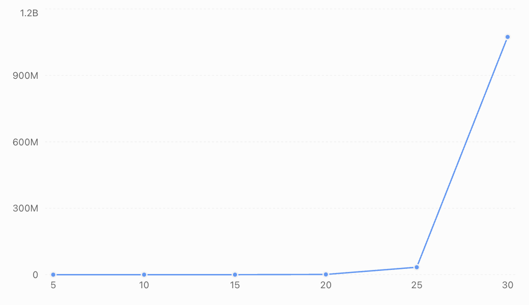
The number of operations doubles whenever the input size increases by one.
This means that even a relatively small increase in input size can cause a very large increase in computational work.
Worked Example 10: Algorithm Processing Time
An algorithm requires 2ⁿ operations.
A computer performs 1 million operations per second.
Estimate the processing time for n = 30.
Step 1: Calculate the number of operations.
T(30) = 2³⁰
T(30) = 1,073,741,824 operations
Step 2: Divide by processing speed.
Time = 1,073,741,824/1,000,000
Time ≈ 1,073.74 seconds
Step 3: Convert to minutes.
Time ≈ 1073.74/60
Time ≈ 17.90 minutes
Now consider n = 40.
T(40) = 2⁴⁰
T(40) = 1,099,511,627,776 operations
Processing time:
1,099,511,627,776/1,000,000 ≈ 1,099,512 seconds
This is approximately:
12.73 days
Increasing the input size from 30 to 40 increases the processing time by a factor of:
2¹⁰ = 1,024
This illustrates why algorithm efficiency is often more important than hardware improvements alone.
Comparing Technological Growth Models
Not every technological relationship is exponential.
Different processes require different mathematical models.
|
Model |
General form |
Possible technology application |
|---|---|---|
|
Linear |
y = mx + b |
Fixed monthly data additions |
|
Quadratic |
y = ax² + bx + c |
Certain computational workloads or cost relationships |
|
Exponential |
y = Abᵗ |
Constant-percentage data growth |
|
Logarithmic |
y = a ln(x) + b |
Some diminishing-return performance relationships |
|
Logistic |
y = K/(1 + Ae⁻ʳᵗ) |
Adoption approaching a finite market size |
Technology adoption and logistic growth
A new technology may initially attract only a small number of users.
As awareness increases, adoption can accelerate.
Eventually, growth may slow as the available market becomes saturated.
This pattern can sometimes be modelled by a logistic function.
Worked Example 11: Technology Adoption
A digital service follows the hypothetical model:
U(t) = 100000/(1 + 19e⁻⁰·⁵ᵗ)
where U(t) is the number of users and t is measured in years.
Calculate the initial number of users and the predicted number after eight years.
Step 1: Calculate the initial users.
At t = 0:
U(0) = 100000/(1 + 19e⁰)
U(0) = 100000/20
U(0) = 5,000 users
Step 2: Calculate users after eight years.
U(8) = 100000/(1 + 19e⁻⁴)
Since e⁻⁴ ≈ 0.0183156:
U(8) ≈ 100000/[1 + 19(0.0183156)]
U(8) ≈ 100000/1.347997
U(8) ≈ 74,184 users
The model predicts approximately 74,184 users after eight years.
The limiting value is 100,000 users.
Why logistic growth may be more realistic
A service cannot acquire more users than the available market allows under a fixed-market assumption.
Exponential growth may describe the early stages of adoption, but it eventually becomes unrealistic if the potential user population is limited.
The logistic model accounts for this constraint.
However, real markets can expand, competitors can enter, and adoption can decline, so the limiting value may change.
Interpreting Technological Data Critically
Exponential models are powerful, but they can be misleading when used without considering the underlying assumptions.
Historical trends do not guarantee future growth
A technology may grow exponentially for several years and then slow because of physical, economic, or practical limitations.
For example, transistor miniaturisation faces challenges involving heat, power consumption, manufacturing complexity, and cost.
Percentage growth can be misleading
A company increasing from 100 to 200 users experiences 100% growth.
A company increasing from 1 million to 1.1 million users experiences 10% growth.
The second company gains far more users, even though its percentage growth is much smaller.
Large numbers need appropriate units
Technological quantities may be expressed in:
-
Kilobytes, megabytes, gigabytes, terabytes, and petabytes.
-
Operations per second.
-
Bits per second.
-
Number of transistors.
-
Number of users or devices.
Always check whether units use decimal or binary prefixes.
For example:
1 TB = 1,000 GB
1 TiB = 1,024 GiB
These are different unit conventions.
Correlation does not establish causation
Two technological trends may increase together without one directly causing the other.
For example, computing capacity and global data volume may both increase over time.
However, their relationship may involve many interacting factors, including demand, software development, storage costs, and network infrastructure.
Evaluating Model Accuracy
A mathematical model should be evaluated using observed data.
A residual is:
Residual = Observed value − Predicted value
Consider a model predicting the number of users of a technology platform.
|
Year |
Observed users |
Predicted users |
Residual |
|---|---|---|---|
|
1 |
1,200 |
1,150 |
+50 |
|
2 |
1,500 |
1,550 |
−50 |
|
3 |
2,100 |
2,000 |
+100 |
|
4 |
2,500 |
2,650 |
−150 |
The residuals help identify how accurately the model represents the observations.
A systematic pattern in the residuals may indicate that the model is missing an important feature of the data.
Overfitting and extrapolation
A model may fit historical data extremely well but perform poorly when predicting future technological developments.
This can occur when:
-
The model is unnecessarily complicated.
-
Growth rates change.
-
The market becomes saturated.
-
New technologies replace older ones.
-
Unexpected economic or regulatory changes occur.
Predictions far beyond the observed time interval are especially uncertain.
Authentic Application: Planning Data Centre Capacity
A technology company currently stores 50 TB of information.
Its data volume has been increasing by approximately 28% per year.
The company wants to estimate future storage requirements.
Part A: Construct a model
Initial storage:
D₀ = 50 TB
Growth factor:
b = 1.28
Therefore:
D(t) = 50(1.28)ᵗ
where t is measured in years.
Part B: Predict storage after five years
D(5) = 50(1.28)⁵
Since:
(1.28)⁵ ≈ 3.435974
D(5) ≈ 50 × 3.435974
D(5) ≈ 171.80 TB
The company should expect approximately 171.8 TB of stored data after five years if the assumed growth rate continues.
Part C: Determine when storage reaches 200 TB
Set:
200 = 50(1.28)ᵗ
Divide by 50:
4 = (1.28)ᵗ
Take natural logarithms:
ln(4) = t ln(1.28)
Therefore:
t = ln(4)/ln(1.28)
t ≈ 5.61 years
The model predicts that the company's stored data will reach 200 TB after approximately 5.61 years.
Part D: Evaluate the model
The company should not assume the 28% growth rate will remain constant indefinitely.
Future storage requirements may be affected by:
-
Data compression.
-
Data retention policies.
-
Changes in customer demand.
-
More efficient software.
-
New products and services.
-
Regulations governing data storage.
-
Changes in the cost of storage.
The exponential model provides a useful planning estimate, but the company should regularly update it using new measurements.
Common Mistakes
Mistake 1: Assuming all technological growth is exponential
Some technologies grow linearly, while others follow logistic or irregular patterns.
Correction: Examine the data before selecting a model.
Mistake 2: Confusing constant increases with constant percentage growth
Adding 100 units per year is linear growth.
Increasing by 20% per year is exponential growth.
Correction: Compare differences and ratios.
Mistake 3: Confusing doubling time with growth rate
Doubling every two years does not mean increasing by 50% annually.
Correction: Use exponential equations to calculate the equivalent growth rate.
Mistake 4: Assuming Moore's Law guarantees future computing improvements
Moore's Law describes a historical technological trend, not a guaranteed physical relationship.
Correction: Consider engineering constraints and changing technological conditions.
Mistake 5: Assuming transistor count and computing performance are identical
More transistors do not automatically produce proportional improvements in processing speed.
Correction: Distinguish hardware component counts from actual performance measurements.
Mistake 6: Ignoring units
Confusing GB and TB, or months and years, can produce large errors.
Correction: Convert units before substituting values.
Mistake 7: Using percentages incorrectly
A growth rate of 15% corresponds to a multiplication factor of 1.15, not 0.15.
Correction: Use b = 1 + r.
Mistake 8: Extrapolating too far
An exponential model may produce unrealistic predictions over long periods.
Correction: State the time interval over which the model is reasonably supported.
Mistake 9: Confusing exponential technology improvement with exponential algorithm complexity
Exponential hardware improvements may be beneficial, while exponential algorithm complexity can make problems increasingly difficult.
Correction: Interpret the quantity represented by the exponential function.
Mistake 10: Ignoring physical and economic limitations
Storage, energy, manufacturing capacity, and market size can limit technological growth.
Correction: Consider alternative models when growth begins to slow.
Key Terms
-
Exponential Growth: Growth involving a constant proportional increase over equal intervals.
-
Growth Factor: Multiplier applied during each time interval.
-
Growth Rate: Percentage or proportional increase over a specified interval.
-
Doubling Time: Time required for a quantity to become twice its original value.
-
Continuous Growth Constant: Parameter describing exponential growth in the model Q(t) = Q₀eᵏᵗ.
-
Moore's Law: Historical observation concerning approximately exponential increases in transistor counts on integrated circuits.
-
Transistor: Semiconductor component used in electronic circuits.
-
Processing Capacity: Measure of the computational work a system can perform.
-
Digital Information: Information represented in digital form.
-
Data Storage: Retention of digital information.
-
Network Traffic: Data transmitted through a network over a specified period.
-
Bandwidth: Capacity of a communication channel to transmit data.
-
Algorithm: Step-by-step computational procedure for solving a problem.
-
Time Complexity: Description of how computational work grows with input size.
-
Exponential Complexity: Computational growth proportional to a function such as 2ⁿ.
-
Compound Annual Growth Rate (CAGR): Equivalent constant annual rate describing an overall change.
-
Logarithmic Scale: Scale that represents multiplicative changes using additive differences.
-
Logarithmic Transformation: Applying logarithms to data to investigate relationships.
-
Technology Adoption: Process by which users or organisations begin using a technology.
-
Logistic Growth: Growth that approaches a limiting value.
-
Market Saturation: Situation in which most potential users or customers have adopted a product or service.
-
Residual: Difference between an observed and predicted value.
-
Extrapolation: Prediction beyond the observed data range.
-
Model Limitation: Restriction on the validity or reliability of a mathematical model.
Key Takeaways
-
Exponential models describe quantities that increase by a constant percentage or multiplication factor.
-
Doubling produces increasingly large absolute changes.
-
Moore's Law describes a historical trend in transistor counts, not a guaranteed future law of computing performance.
-
Digital storage and information growth can sometimes be modelled exponentially.
-
Constant ratios in equally spaced data suggest exponential growth.
-
Natural logarithms allow us to calculate growth constants, doubling times, and when capacity thresholds will be reached.
-
Logarithmic transformations can help reveal exponential trends.
-
Network capacity planning is an important application of exponential models.
-
Exponential algorithm complexity describes rapidly increasing computational requirements.
-
Logistic models may be more appropriate when technology adoption approaches a limited market size.
-
Historical technological growth does not guarantee future exponential growth.
-
Reliable modelling requires appropriate units, accurate data, and careful evaluation of assumptions.
Check Your Understanding
Questions
Question 1: Identifying Exponential Growth
Determine which of the following represent exponential growth.
a) A computer's capacity increases by 200 units each year.
b) A data centre's storage requirement increases by 15% each year.
c) A server's workload doubles every four months.
d) A company's number of employees increases by 20 each year.
Question 2: Computing Capacity
A hypothetical computing system begins with a capacity of 500 units and doubles every two years.
Calculate its capacity after eight years.
Question 3: Data Growth
A research organisation stores 20 TB of data.
Its stored data increases by 25% annually.
Calculate the amount after four years.
Question 4: Growth Factor
A digital service increases its number of users by 18% each month.
Determine the monthly growth factor and write a model if the initial number of users is 3,000.
Question 5: Doubling Time
A technology's capacity doubles every three years.
Write an exponential model if its initial capacity is 1,200 units.
Question 6: Continuous Growth
A computing capability follows:
C(t) = 800e⁰·³ᵗ
Calculate its value after five years.
Question 7: Growth Constant
A technology doubles in capacity every 2.5 years.
Calculate its continuous growth constant.
Question 8: Identifying a Trend
A technology company records the following data.
|
Year |
Capacity |
|---|---|
|
0 |
100 |
|
1 |
140 |
|
2 |
196 |
|
3 |
274.4 |
Determine whether a linear or exponential model is more appropriate and explain why.
Question 9: CAGR
A digital platform increases from 5,000 users to 20,000 users over five years.
Calculate its compound annual growth rate.
Question 10: Network Capacity
A network currently carries 600 GB of traffic per day.
Traffic grows by 20% annually.
Calculate the predicted daily traffic after six years.
Question 11: Reaching a Threshold
A company's data storage requirement is 40 TB and increases by 30% per year.
How long will it take to reach 100 TB?
Question 12: Algorithm Complexity
An algorithm requires 2ⁿ operations.
Calculate the number of operations for n = 15 and n = 20.
By what factor does the number of operations increase?
Question 13: Technology Adoption
A service follows:
U(t) = 50000/(1 + 9e⁻⁰·⁴ᵗ)
Determine the limiting number of users and the initial number of users.
Question 14: Interpreting Moore's Law
Explain why a doubling in transistor count does not necessarily mean a doubling in computer processing speed.
Question 15: Critical Modelling
A company's stored data has increased by 40% annually for three years.
Explain why using the same growth rate to predict storage requirements 30 years into the future may be unreliable.
Fully Worked Answers
Answer 1: Identifying Exponential Growth
a) Linear — the capacity increases by a fixed amount.
b) Exponential — the storage requirement increases by a constant percentage.
c) Exponential — the workload doubles over equal time intervals.
d) Linear — the number of employees increases by a fixed amount.
Answer 2: Computing Capacity
Initial capacity = 500 units
Doubling time = 2 years
Elapsed time = 8 years
Model:
C(t) = 500 × 2^(t/2)
Substitute:
C(8) = 500 × 2⁴
C(8) = 500 × 16
C(8) = 8,000 units
Answer 3: Data Growth
Initial data = 20 TB
Growth rate = 25%
Growth factor = 1.25
Model:
D(t) = 20(1.25)ᵗ
After four years:
D(4) = 20(1.25)⁴
D(4) = 20(2.44140625)
D(4) ≈ 48.83 TB
Answer 4: Growth Factor
Growth rate = 18% = 0.18
Growth factor:
b = 1 + 0.18
b = 1.18
Initial users = 3,000
Model:
U(t) = 3000(1.18)ᵗ
where t is measured in months.
Answer 5: Doubling Time
Initial capacity = 1,200 units
Doubling time = 3 years
Model:
C(t) = 1200 × 2^(t/3)
where t is measured in years.
Answer 6: Continuous Growth
Given:
C(t) = 800e⁰·³ᵗ
At t = 5:
C(5) = 800e¹·⁵
Since e¹·⁵ ≈ 4.481689:
C(5) ≈ 800 × 4.481689
C(5) ≈ 3,585.35 units
Answer 7: Growth Constant
Doubling time = 2.5 years
Use:
k = ln(2)/T
k = 0.693147/2.5
k ≈ 0.2773 year⁻¹
Answer 8: Identifying a Trend
Calculate ratios:
140/100 = 1.4
196/140 = 1.4
274.4/196 = 1.4
The ratios are constant.
Therefore, an exponential model is appropriate.
Initial capacity = 100
Growth factor = 1.4
C(t) = 100(1.4)ᵗ
Answer 9: CAGR
Initial users = 5,000
Final users = 20,000
Time = 5 years
CAGR = (20000/5000)^(1/5) − 1
CAGR = 4^(1/5) − 1
CAGR ≈ 0.319508
CAGR ≈ 31.95% per year
Answer 10: Network Capacity
Initial traffic = 600 GB/day
Growth rate = 20%
Model:
T(t) = 600(1.2)ᵗ
After six years:
T(6) = 600(1.2)⁶
T(6) = 600(2.985984)
T(6) ≈ 1,791.59 GB/day
Answer 11: Reaching a Threshold
Model:
D(t) = 40(1.3)ᵗ
Set D(t) = 100:
100 = 40(1.3)ᵗ
Divide by 40:
2.5 = (1.3)ᵗ
Take logarithms:
ln(2.5) = t ln(1.3)
Therefore:
t = ln(2.5)/ln(1.3)
t ≈ 3.49 years
The storage requirement reaches 100 TB after approximately 3.49 years under the model.
Answer 12: Algorithm Complexity
For n = 15:
T(15) = 2¹⁵
T(15) = 32,768 operations
For n = 20:
T(20) = 2²⁰
T(20) = 1,048,576 operations
Factor of increase:
1,048,576/32,768 = 32
The number of operations increases by a factor of 32.
Answer 13: Technology Adoption
Given:
U(t) = 50000/(1 + 9e⁻⁰·⁴ᵗ)
The limiting value is:
50,000 users
At t = 0:
U(0) = 50000/(1 + 9)
U(0) = 50000/10
Initial users = 5,000
Answer 14: Interpreting Moore's Law
Transistor count measures the number of transistors on a chip.
Processing speed depends on additional factors such as processor architecture, memory access, clock frequency, parallel processing, software efficiency, and power limitations.
Therefore, doubling the number of transistors does not guarantee that processing speed doubles.
Answer 15: Critical Modelling
An annual growth rate of 40% may describe the company's recent storage requirements accurately.
However, projecting the same rate over 30 years assumes that the underlying conditions remain unchanged.
In reality, storage growth may be affected by changes in customer demand, compression technology, data retention policies, storage costs, and business activity.
The model may therefore overestimate or underestimate long-term requirements.
A more reliable approach would involve updating the model regularly and comparing several possible growth scenarios.
Final Reflection
Exponential models provide a valuable mathematical framework for understanding technological development.
They explain why repeated doubling can produce enormous changes, why digital information requirements can increase rapidly, and why network infrastructure must be planned with future growth in mind.
They also help us analyse computational complexity, estimate doubling times, and compare historical technological trends.
However, not all technological processes grow exponentially, and even those that do may eventually slow or change direction.
The most important skill is not simply recognising an exponential curve, but understanding what the model represents, interpreting its parameters, using it to solve realistic problems, and recognising when its predictions may no longer be reliable.