Applications and Connections

1. Finance Applications

Introduction

Mathematics plays an essential role in financial decision-making. Whether we are saving money, investing for the future, borrowing to purchase a home, or comparing different loan offers, mathematical models help us understand how money changes over time.

Consider the following questions:

• How much will $5,000 become after 10 years in a savings account?

• Is an investment offering 6% annual interest necessarily better than one offering 5.9% interest compounded monthly?

• How much should someone save each month to reach a financial goal?

• Why can a long-term loan cost considerably more than the original amount borrowed?

• How can we compare investments with different growth rates, fees, and risks?

These questions involve exponential functions, geometric sequences, logarithms, percentages, and mathematical modelling.

In this lesson, we will explore how mathematical models are used in personal finance, investment analysis, loan repayments, and the interpretation of financial data.

The goal is not simply to calculate financial values, but to understand what those calculations mean and how they can support informed decisions.

The Time Value of Money

One of the most important ideas in finance is the time value of money.

Money available today can be invested to earn a return, so it may be worth more than the same nominal amount received in the future.

For example, $1,000 invested at an annual return of 5% becomes:

After one year:

1,000 × 1.05 = $1,050

After two years:

1,050 × 1.05 = $1,102.50

After three years:

1,102.50 × 1.05 = $1,157.63

The amount increases because each year's growth is calculated using the previous year's balance.

This is the principle of compound interest.

The time value of money also depends on inflation, risk, and the opportunity cost of using money for one purpose rather than another.

Simple Interest

Simple interest is calculated only on the original principal.

The formula is:

I = Prt

Where:

• I = interest earned.

• P = principal or original amount.

• r = annual interest rate as a decimal.

• t = time in years.

The final amount is:

A = P(1 + rt)

Worked Example 1: Simple Interest

An investor deposits $4,000 at 5% simple annual interest for six years.

Calculate the interest and final amount.

Step 1: Identify the values.

P = 4000

r = 0.05

t = 6

Step 2: Calculate interest.

I = 4000 × 0.05 × 6

I = 1200

Step 3: Calculate the final amount.

A = 4000 + 1200

Final amount = $5,200

Simple interest produces linear growth because the same amount of interest is earned each year.

Compound Interest

Compound interest is calculated on the principal and previously accumulated interest.

With annual compounding:

A = P(1 + r)ⁿ

Where:

• A = final amount.

• P = initial principal.

• r = annual interest rate as a decimal.

• n = number of years.

Unlike simple interest, compound interest produces exponential growth.

Visualising compound interest

Worked Example 2: Annual Compound Interest

An investor deposits $5,000 into an account paying 6% interest compounded annually.

Calculate the balance after 10 years.

Step 1: Identify the values.

P = 5000

r = 0.06

n = 10

Step 2: Substitute.

A = 5000(1.06)¹⁰

Step 3: Evaluate.

(1.06)¹⁰ ≈ 1.790848

A ≈ 5000 × 1.790848

A ≈ $8,954.24

Step 4: Calculate the interest earned.

Interest = 8954.24 − 5000

Interest ≈ $3,954.24

The investment earns approximately $3,954.24 over 10 years.

Simple Interest Versus Compound Interest

Consider $5,000 invested at 6% annually.

Simple interest increases by a constant amount each year.

Compound interest increases by a constant percentage each year.

Over longer periods, the difference becomes increasingly significant.

Compounding More Than Once Per Year

Interest may be compounded annually, semiannually, quarterly, monthly, or daily.

The general compound interest formula is:

A = P(1 + r/m)^(mt)

Where:

• P = principal.

• r = nominal annual interest rate.

• m = number of compounding periods per year.

• t = time in years.

The interest rate per compounding period is r/m.

The total number of compounding periods is mt.

Worked Example 3: Monthly Compounding

An investment of $8,000 earns 4.8% annual interest compounded monthly for five years.

Calculate the final amount.

P = 8000

r = 0.048

m = 12

t = 5

Substitute:

A = 8000(1 + 0.048/12)^(12 × 5)

A = 8000(1.004)⁶⁰

A ≈ 8000(1.27064)

A ≈ $10,165.12

The final amount is approximately $10,165.12.

The interest earned is approximately $2,165.12.

Continuous Compounding

Continuous compounding represents the limiting case as interest is compounded increasingly frequently.

The formula is:

A = Peʳᵗ

Where e ≈ 2.71828.

Worked Example 4: Continuous Compounding

A deposit of $10,000 earns 5% annual interest compounded continuously for eight years.

A = 10000e^(0.05 × 8)

A = 10000e⁰·⁴

A ≈ 10000(1.491825)

A ≈ $14,918.25

The interest earned is approximately $4,918.25.

Comparing Compounding Frequencies

For a nominal annual interest rate of 6%, an investment of $10,000 produces different balances after one year.

More frequent compounding increases the final amount when the nominal rate is positive.

However, the additional benefit becomes smaller as the frequency increases.

Continuous compounding does not mean unlimited interest. It produces a finite limiting value for any fixed principal, interest rate, and time period.

Effective Annual Interest Rate

Two financial products may advertise the same nominal annual interest rate but use different compounding frequencies.

To compare them fairly, we calculate the effective annual rate (EAR).

The formula is:

EAR = (1 + r/m)ᵐ − 1

Where:

• r = nominal annual interest rate.

• m = number of compounding periods per year.

For continuous compounding:

EAR = eʳ − 1

Worked Example 5: Comparing Savings Accounts

Bank A offers 5% interest compounded annually.

Bank B offers 4.9% interest compounded monthly.

Which account provides the higher effective annual rate?

Bank A

EAR = 0.05

EAR = 5%

Bank B

EAR = (1 + 0.049/12)¹² − 1

EAR ≈ 0.050115

EAR ≈ 5.012%

Conclusion

Bank B offers a slightly higher effective annual rate.

Although Bank B advertises a lower nominal rate, monthly compounding produces a marginally higher annual return.

This comparison assumes the same conditions and excludes fees, taxes, withdrawal restrictions, and other differences.

Investment Growth Over Time

Investments may grow through interest, dividends, capital appreciation, or a combination of these.

For a constant effective annual return r:

V(t) = V₀(1 + r)ᵗ

Where:

• V₀ = initial investment.

• r = effective annual return.

• t = number of years.

Worked Example 6: Comparing Investment Growth

Two investments begin with $10,000.

Investment A earns 4% annually.

Investment B earns 7% annually.

Compare their values after 20 years.

Investment A:

A = 10000(1.04)²⁰

A ≈ $21,911.23

Investment B:

B = 10000(1.07)²⁰

B ≈ $38,696.84

Difference:

38,696.84 − 21,911.23

Difference ≈ $16,785.61

A difference of three percentage points in annual growth produces a substantial difference over 20 years.

However, higher expected returns are often associated with greater uncertainty or risk. Real investment returns are not generally constant or guaranteed.

The Rule of 72

The Rule of 72 provides a quick estimate of the time required for an investment to double.

Doubling time ≈ 72 ÷ annual growth rate (%)

For example, at 6% annual growth:

Doubling time ≈ 72/6

Doubling time ≈ 12 years

The exact doubling time for annual compounding is:

t = ln(2)/ln(1 + r)

At 6%:

t = ln(2)/ln(1.06)

t ≈ 11.90 years

The Rule of 72 provides a convenient approximation, but logarithms give a more accurate result.

Solving for Time Using Logarithms

Compound interest problems sometimes ask how long an investment must grow to reach a target amount.

Start with:

A = P(1 + r)ᵗ

Divide by P:

A/P = (1 + r)ᵗ

Take natural logarithms:

ln(A/P) = t ln(1 + r)

Therefore:

t = ln(A/P)/ln(1 + r)

Worked Example 7: Reaching a Savings Goal

An investor deposits $6,000 at 5% annual compound interest.

How long will it take to reach $10,000?

10000 = 6000(1.05)ᵗ

Divide by 6000:

1.666667 = (1.05)ᵗ

Take natural logarithms:

ln(1.666667) = t ln(1.05)

t = ln(1.666667)/ln(1.05)

t ≈ 10.47 years

If interest is credited only at the end of each year, the balance first reaches or exceeds $10,000 after 11 complete years.

Regular Savings Contributions

Many people invest regularly rather than depositing a single amount.

For equal payments made at the end of each period, the future value of an ordinary annuity is:

FV = PMT[(1 + i)ⁿ − 1]/i

Where:

• FV = future value.

• PMT = payment each period.

• i = interest rate per period.

• n = number of payments.

The formula assumes that payments and compounding occur at the same regular intervals and that the interest rate remains constant.

Worked Example 8: Monthly Retirement Savings

A person invests $250 at the end of each month for 20 years.

The account earns a nominal annual interest rate of 6%, compounded monthly.

Calculate the future value.

Step 1: Identify the values.

PMT = 250

Monthly rate:

i = 0.06/12 = 0.005

Number of payments:

n = 20 × 12 = 240

Step 2: Substitute.

FV = 250[(1.005)²⁴⁰ − 1]/0.005

Step 3: Evaluate.

(1.005)²⁴⁰ ≈ 3.31020

FV ≈ 250(2.31020/0.005)

FV ≈ $115,510.22

Step 4: Calculate total contributions.

250 × 240 = $60,000

Step 5: Calculate investment growth.

115510.22 − 60000

Growth ≈ $55,510.22

The account grows to approximately $115,510, of which $60,000 comes from contributions and the remainder from compounded returns.

This example assumes fixed returns and ignores taxes, fees, and inflation.

Understanding Loans and Repayments

A loan allows someone to borrow money and repay it over time, usually with interest.

Common examples include:

• Home mortgages.

• Car loans.

• Personal loans.

• Student loans.

• Business loans.

Important loan terms include:

Principal: The amount originally borrowed.

Interest rate: The cost of borrowing, expressed as a percentage.

Loan term: The period over which the loan is repaid.

Repayment: The amount paid at each scheduled interval.

Outstanding balance: The amount still owed at a particular time.

How amortising loans work

An amortising loan is repaid through regular payments that cover interest and reduce the principal.

In a standard fixed-rate, fully amortising loan, the payments remain equal, but the proportion allocated to interest and principal changes over time.

At the beginning, the outstanding balance is relatively large, so the interest component is large.

As the principal decreases, less interest is charged each period, and more of each payment reduces the remaining principal.

The Loan Repayment Formula

For a loan with equal payments at the end of each period:

PMT = PV × i/[1 − (1 + i)⁻ⁿ]

Where:

• PMT = regular repayment.

• PV = present value, or amount borrowed.

• i = interest rate per repayment period.

• n = total number of repayments.

The formula assumes a constant interest rate, regular payment intervals, and no additional fees.

For monthly repayments with a nominal annual rate r compounded monthly:

i = r/12

n = 12t

where t is the loan term in years.

Worked Example 9: Calculating a Monthly Loan Repayment

A person borrows $20,000 at a nominal annual interest rate of 6%, compounded monthly.

The loan is repaid through equal monthly payments over five years.

Calculate the monthly repayment.

Step 1: Identify the values.

PV = 20000

Annual rate = 0.06

Monthly rate:

i = 0.06/12 = 0.005

Number of payments:

n = 5 × 12 = 60

Step 2: Substitute into the repayment formula.

PMT = 20000 × 0.005/[1 − (1.005)⁻⁶⁰]

Step 3: Evaluate.

(1.005)⁻⁶⁰ ≈ 0.74137

PMT ≈ 100/(1 − 0.74137)

PMT ≈ $386.66 per month

The borrower pays approximately $386.66 each month. The lender may adjust the final payment slightly because of rounding.

Calculating total interest

Total payments, using the rounded monthly payment:

60 × 386.66 = $23,199.60

Total interest:

23,199.60 − 20,000

Total interest ≈ $3,199.60

The borrower repays approximately $3,200 more than the original loan amount.

Understanding Loan Amortisation

An amortisation schedule shows how each repayment is divided between interest and principal.

For each period:

Interest = Outstanding balance × Periodic interest rate

Principal repaid = Payment − Interest

New balance = Previous balance − Principal repaid

Equivalently:

New balance = Previous balance(1 + i) − Payment

Worked Example 10: First Three Loan Payments

Consider the $20,000 loan with monthly repayments of approximately $386.66 and monthly interest rate 0.005.

First payment

Interest:

20000 × 0.005 = $100.00

Principal repaid:

386.66 − 100.00 = $286.66

New balance:

20000 − 286.66 = $19,713.34

Second payment

Interest:

19713.34 × 0.005 ≈ $98.57

Principal repaid:

386.66 − 98.57 = $288.09

New balance:

19713.34 − 288.09 = $19,425.25

Third payment

Interest:

19425.25 × 0.005 ≈ $97.13

Principal repaid:

386.66 − 97.13 = $289.53

New balance:

19425.25 − 289.53 = $19,135.72

Values are rounded to the nearest cent. An actual lender's amortisation schedule may differ slightly because of its rounding conventions.

Notice that the interest component decreases while the principal component increases.

This is why the outstanding loan balance decreases slowly at first and more quickly later.

Visualising Loan Repayment

The following graph shows an illustrative $20,000 loan at 6% nominal annual interest, repaid monthly over five years.

The graph curves downward because the amount of principal repaid each month increases as the interest component decreases.

Comparing Loan Terms

A longer loan term usually reduces the required monthly payment, but increases the total interest paid when the interest rate is unchanged.

Consider a $30,000 loan at a nominal annual interest rate of 6%, compounded monthly.

The seven-year loan has the lowest monthly repayment, but the highest total interest cost.

The three-year loan has a higher monthly repayment but a lower total borrowing cost.

Interpreting the trade-off

A borrower must consider both affordability and overall cost.

A smaller monthly payment may be easier to manage, but it does not necessarily mean the loan is cheaper.

The best loan is not simply the loan with the lowest monthly repayment.

Other important factors include fees, effective interest rates, early repayment conditions, and whether the rate is fixed or variable.

Calculating the Outstanding Loan Balance

After several repayments, the outstanding balance can be calculated using:

Bₖ = PV(1 + i)ᵏ − PMT[(1 + i)ᵏ − 1]/i

Where:

• Bₖ = balance after k payments.

• PV = original loan amount.

• i = interest rate per period.

• PMT = regular payment.

• k = number of payments made.

The first term represents how much the original loan would have grown through interest.

The second term represents the accumulated effect of repayments.

Worked Example 11: Outstanding Balance

A borrower takes out a $10,000 loan at 1% interest per month and makes payments of $300 at the end of each month.

Find the outstanding balance immediately after 12 payments.

PV = 10000

i = 0.01

PMT = 300

k = 12

Substitute:

B₁₂ = 10000(1.01)¹² − 300[(1.01)¹² − 1]/0.01

Since:

(1.01)¹² ≈ 1.126825

B₁₂ ≈ 11268.25 − 300(12.6825)

B₁₂ ≈ 11268.25 − 3804.75

B₁₂ ≈ $7,463.50

The borrower still owes approximately $7,463.50 after 12 payments.

The exact balance depends on the lender's interest and rounding rules.

Present Value and Discounting

Compound interest calculates how money grows into the future.

Present value works in the opposite direction.

It calculates how much a future amount is worth today under an assumed discount rate.

For annual compounding:

PV = FV/(1 + r)ⁿ

Where:

• PV = present value.

• FV = future value.

• r = discount rate per period.

• n = number of periods.

Worked Example 12: Present Value

An investment is expected to pay $15,000 in five years.

If the appropriate annual discount rate is 6%, calculate its present value.

PV = 15000/(1.06)⁵

PV = 15000/1.338226

PV ≈ $11,208.87

This means that approximately $11,208.87 invested today at 6% annually would grow to $15,000 after five years.

The present value depends on the discount rate selected.

Comparing Financial Models

Financial situations may involve linear, exponential, and annuity-based models.

Choosing the correct model

Before selecting a formula, ask:

1. Is the interest simple or compounded?

2. Are payments made once or repeatedly?

3. Are payments made at the beginning or end of each period?

4. What is the interest rate per period?

5. How many periods are involved?

6. Is the rate fixed or variable?

7. Are fees, taxes, inflation, or other factors relevant?

Using the wrong model can produce a significantly incorrect financial result.

Inflation and Purchasing Power

Inflation refers to an increase in the general price level over time.

When prices rise, the purchasing power of a fixed amount of money decreases.

If inflation remains constant at rate f per year:

Future price = Current price × (1 + f)ᵗ

The purchasing power of a future nominal amount, expressed in today's money, is:

Real value = Future nominal value/(1 + f)ᵗ

Worked Example 13: Inflation

An item costs $1,000 today.

Assume prices increase by 3% annually for 10 years.

Calculate its expected price after 10 years.

Future price = 1000(1.03)¹⁰

Future price ≈ 1000(1.343916)

Future price ≈ $1,343.92

An item costing $1,000 today would cost approximately $1,343.92 after 10 years under this assumption.

Real Investment Returns

Suppose an investment earns an effective nominal annual return of 7%, while inflation is 3%.

The exact real annual return is:

Real return = (1 + nominal return)/(1 + inflation) − 1

Real return = 1.07/1.03 − 1

Real return ≈ 0.038835

Real return ≈ 3.88%

Although the investment grows by 7% in nominal terms, its purchasing power increases by approximately 3.88% per year.

This assumes the stated rates remain constant and ignores taxes and fees.

Interpreting Financial Data

Financial data should be interpreted mathematically rather than simply accepted at face value.

Important measures include:

• Absolute change.

• Percentage change.

• Compound annual growth rate.

• Effective interest rate.

• Total interest paid.

• Real return after inflation.

• Volatility and uncertainty.

Percentage Change

Percentage change = [(New value − Old value)/Old value] × 100%

Suppose an investment increases from $8,000 to $9,200.

Percentage change:

(9200 − 8000)/8000 × 100%

= 1200/8000 × 100%

Percentage increase = 15%

Compound Annual Growth Rate (CAGR)

CAGR measures the constant annual growth rate that would produce the same beginning and ending values over a specified period.

CAGR = (Final value/Initial value)^(1/n) − 1

Worked Example 14: Calculating CAGR

An investment grows from $12,000 to $18,000 over six years.

Calculate its compound annual growth rate.

CAGR = (18000/12000)^(1/6) − 1

CAGR = 1.5^(1/6) − 1

CAGR ≈ 0.069913

CAGR ≈ 6.99% per year

This means the investment experienced the same overall growth as an investment increasing at approximately 6.99% every year.

It does not mean the actual return was 6.99% in each individual year.

Interpreting Investment Performance Graphs

Consider an investment with the following year-end values.

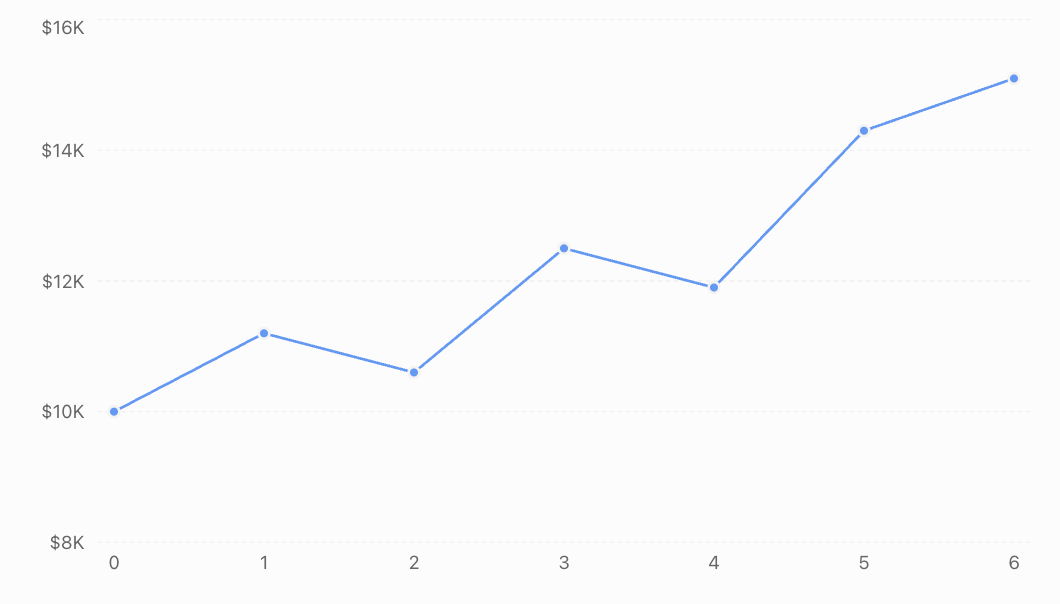
The investment increases overall from $10,000 to $15,100.

Total return:

(15100 − 10000)/10000 × 100%

Total return = 51%

However, the graph shows that growth was not constant.

The investment experienced declines in some years.

This illustrates an important limitation of using a single constant-rate exponential model for investment performance.

Mathematical questions to ask

When interpreting a financial graph, consider:

• Is the vertical axis scaled appropriately?

• Are values nominal or inflation-adjusted?

• Does the graph include fees and dividends?

• Are the time intervals consistent?

• Does the graph show a long enough period?

• Is the reported return an average, a compound annual rate, or a single-period return?

• Does the model account for uncertainty and risk?

A graph showing strong historical growth does not guarantee similar future performance.

Financial Risk and Mathematical Modelling

Financial models often assume that interest rates and investment returns remain constant. Real financial markets are more complicated.

Investment values can fluctuate, interest rates can change, and unexpected events can affect financial outcomes.

Expected Return

Suppose an investment has three possible annual outcomes.

The expected return is calculated using a weighted average:

E(R) = Σ[pᵢ × Rᵢ]

Substitute:

E(R) = 0.25(15%) + 0.50(6%) + 0.25(−8%)

E(R) = 3.75% + 3% − 2%

Expected return = 4.75%

This does not mean the investment will earn exactly 4.75%.

It represents the probability-weighted average return under the assumed outcomes.

Risk and Return

Two investments may have the same expected return but different levels of risk.

For example, one investment might consistently earn returns close to 5%, while another experiences large gains and losses.

Measures such as standard deviation can help describe the variability of returns.

Financial decisions should therefore consider both expected return and uncertainty.

Authentic Application: Comparing Two Savings Plans

A student wants to save money for university expenses over the next 10 years.

Two savings plans are available.

Plan A

• Initial deposit: $5,000

• Nominal annual interest rate: 4.5%

• Compounded annually

• No additional contributions

Plan B

• Initial deposit: $5,000

• Nominal annual interest rate: 4.2%

• Compounded monthly

• No additional contributions

Which plan produces the larger balance after 10 years?

Step 1: Calculate Plan A

A = 5000(1.045)¹⁰

A ≈ 5000(1.55297)

Plan A ≈ $7,764.85

Step 2: Calculate Plan B

A = 5000(1 + 0.042/12)¹²⁰

A = 5000(1.0035)¹²⁰

A ≈ 5000(1.52089)

Plan B ≈ $7,604.45

Step 3: Compare the results

Difference:

7764.85 − 7604.45

Difference ≈ $160.40

Plan A produces approximately $160 more over 10 years under the stated assumptions.

Step 4: Interpret the result

Although Plan B compounds more frequently, Plan A offers a sufficiently higher nominal interest rate to produce a larger final balance.

This demonstrates why comparing compounding frequency alone is not enough.

A complete comparison should consider effective annual rates, fees, account conditions, and whether the advertised rates are guaranteed.

Authentic Application: Comparing Two Loan Offers

A borrower needs $25,000 to purchase a vehicle.

Two lenders offer fixed-rate loans with monthly compounding and payments.

Loan A

Monthly rate:

i = 0.055/12

Number of payments:

n = 60

Monthly repayment:

PMT = 25000(0.055/12)/[1 − (1 + 0.055/12)⁻⁶⁰]

PMT ≈ $477.53

Total repayment:

Approximately $28,651.80

Total interest:

Approximately $3,651.80

Loan B

Monthly rate:

i = 0.062/12

Number of payments:

n = 48

Monthly repayment:

PMT = 25000(0.062/12)/[1 − (1 + 0.062/12)⁻⁴⁸]

PMT ≈ $589.46

Total repayment:

Approximately $28,294.08

Total interest:

Approximately $3,294.08

Comparing the loans

Loan A has a lower monthly repayment.

Loan B has a higher monthly repayment but a lower total interest cost because it is repaid more quickly.

The choice depends on the borrower's budget, financial priorities, and the full loan conditions.

The comparison excludes fees, insurance, and other possible charges.

Common Mistakes

Mistake 1: Confusing simple and compound interest

Simple interest is calculated only on the original principal.

Compound interest includes interest earned on previous interest.

Correction: Identify the interest calculation method before choosing a formula.

Mistake 2: Using a percentage instead of a decimal

Substituting 5 instead of 0.05 produces an incorrect result.

Correction: Divide percentage rates by 100.

Mistake 3: Mixing time units

Using an annual interest rate with monthly periods without conversion gives incorrect results.

Correction: Ensure the interest rate and number of periods use consistent units.

Mistake 4: Assuming more frequent compounding always means a better investment

A higher nominal rate with less frequent compounding may outperform a lower rate with more frequent compounding.

Correction: Compare effective annual rates.

Mistake 5: Confusing loan repayment with interest expense

Each loan repayment generally includes principal and interest.

Correction: Use an amortisation schedule to distinguish the components.

Mistake 6: Comparing loans only by monthly repayment

A longer loan may have smaller monthly payments but greater total interest.

Correction: Compare the full repayment cost and loan conditions.

Mistake 7: Ignoring inflation

An investment may increase in nominal value while gaining little purchasing power.

Correction: Calculate real returns where appropriate.

Mistake 8: Assuming investment returns are guaranteed

Constant-rate models are mathematical simplifications.

Correction: Consider variability, uncertainty, fees, and risk.

Mistake 9: Treating CAGR as the actual return every year

CAGR represents an equivalent constant annual rate.

Correction: Examine individual annual returns as well as overall growth.

Mistake 10: Assuming a lower advertised loan rate always means a cheaper loan

Fees, compounding conventions, and repayment terms can affect the total cost.

Correction: Compare effective rates and total borrowing costs on a consistent basis.

Key Terms

• Principal: The original amount invested or borrowed.

• Simple Interest: Interest calculated only on the original principal.

• Compound Interest: Interest calculated on the principal and accumulated interest.

• Compounding Period: The interval at which interest is added.

• Nominal Interest Rate: The stated annual interest rate before adjusting for compounding frequency.

• Effective Annual Rate (EAR): The actual annual rate after accounting for compounding.

• Continuous Compounding: The limiting form of compounding as the frequency increases without bound.

• Future Value: The value of an investment or series of payments at a future date.

• Present Value: The current equivalent value of a future payment or series of payments under a specified discount rate.

• Annuity: A series of regular payments.

• Ordinary Annuity: An annuity with payments at the end of each period.

• Amortisation: The gradual repayment of a loan through scheduled payments.

• Outstanding Balance: The remaining amount owed on a loan.

• Loan Term: The period over which a loan is repaid.

• Inflation: A general increase in prices over time.

• Purchasing Power: The amount of goods and services that money can buy.

• Nominal Return: Investment return before adjusting for inflation.

• Real Return: Investment return adjusted for inflation.

• Compound Annual Growth Rate (CAGR): The constant annual growth rate equivalent to an observed overall change.

• Expected Return: A probability-weighted average of possible returns.

• Financial Risk: Uncertainty about financial outcomes.

• Discount Rate: The rate used to convert future amounts into present values.

Key Takeaways

• Simple interest produces linear growth, while compound interest produces exponential growth.

• Compound interest allows interest to earn additional interest.

• More frequent compounding increases returns when the nominal rate is fixed and positive.

• Effective annual rates allow fairer comparisons between different compounding frequencies.

• Natural exponential functions model continuous compounding.

• Logarithms can be used to solve for investment time and growth rates.

• Regular contributions can be modelled using annuity formulas.

• Fixed-rate amortising loans involve repayments that cover both interest and principal.

• Longer loan terms generally reduce monthly repayments but increase total interest costs at a fixed rate.

• Present value converts future payments into their equivalent value today.

• Inflation reduces purchasing power.

• CAGR describes equivalent annual growth, not necessarily the actual return in each year.

• Financial decisions should consider mathematical results, assumptions, costs, and uncertainty.

Check Your Understanding

Questions

Question 1: Simple Interest

An investor deposits $3,000 at 4% simple annual interest for five years.

Calculate the interest earned and final amount.

Question 2: Compound Interest

An investment of $4,500 earns 5% interest compounded annually.

Calculate the balance after eight years.

Question 3: Quarterly Compounding

A deposit of $6,000 earns 4.8% annual interest compounded quarterly for three years.

Calculate the final amount.

Question 4: Continuous Compounding

An investment of $8,000 earns 3.5% interest compounded continuously for 12 years.

Calculate its final value.

Question 5: Effective Annual Rate

A bank offers 6% nominal annual interest compounded monthly.

Calculate the effective annual interest rate.

Question 6: Comparing Investments

Investment A earns 5% compounded annually.

Investment B earns 4.9% compounded monthly.

Which has the higher effective annual rate?

Question 7: Investment Growth

An investment grows from $10,000 to $16,000 over seven years.

Calculate its compound annual growth rate.

Question 8: Doubling Time

An investment earns 7% interest compounded annually.

How long will it take to double?

Question 9: Regular Savings

A person deposits $200 at the end of every month into an account earning 6% nominal annual interest compounded monthly.

Calculate the value after 10 years.

Question 10: Loan Repayment

A borrower takes out a $15,000 loan at 6% nominal annual interest compounded monthly.

The loan is repaid over four years through equal monthly payments.

Calculate the monthly repayment.

Question 11: Loan Interest

Using your answer to Question 10, estimate the total interest paid over the four-year term.

Question 12: Amortisation

A borrower owes $12,000 on a loan charging 1% interest per month.

The next monthly repayment is $400.

Calculate the interest, principal repayment, and new outstanding balance.

Question 13: Inflation

An item costs $2,000 today.

If inflation averages 3% annually, calculate its expected price after 15 years.

Question 14: Real Return

An investment earns a nominal effective annual return of 8%.

Inflation is 3% annually.

Calculate the real annual return.

Question 15: Financial Decision-Making

A borrower is offered two loans for $20,000.

Loan A has monthly repayments of $400 for 60 months.

Loan B has monthly repayments of $480 for 48 months.

Which loan has the lower total repayment cost? Explain why the lower monthly repayment is not necessarily the better financial choice.

Fully Worked Answers

Answer 1: Simple Interest

I = Prt

I = 3000 × 0.04 × 5

I = $600

Final amount:

A = 3000 + 600

A = $3,600

Answer 2: Compound Interest

A = P(1 + r)ⁿ

A = 4500(1.05)⁸

A ≈ 4500(1.477455)

A ≈ $6,648.55

Answer 3: Quarterly Compounding

P = 6000

r = 0.048

m = 4

t = 3

A = 6000(1 + 0.048/4)^(4 × 3)

A = 6000(1.012)¹²

A ≈ $6,923.37

Answer 4: Continuous Compounding

A = Peʳᵗ

A = 8000e^(0.035 × 12)

A = 8000e⁰·⁴²

A ≈ 8000(1.521962)

A ≈ $12,175.70

Answer 5: Effective Annual Rate

EAR = (1 + r/m)ᵐ − 1

EAR = (1 + 0.06/12)¹² − 1

EAR = (1.005)¹² − 1

EAR ≈ 0.061678

EAR ≈ 6.168%

Answer 6: Comparing Investments

Investment A:

EAR = 5%

Investment B:

EAR = (1 + 0.049/12)¹² − 1

EAR ≈ 5.012%

Investment B has the higher effective annual rate, although the difference is small.

Answer 7: Investment Growth

CAGR = (Final/Initial)^(1/n) − 1

CAGR = (16000/10000)^(1/7) − 1

CAGR = 1.6^(1/7) − 1

CAGR ≈ 0.06945

CAGR ≈ 6.95% per year

Answer 8: Doubling Time

2P = P(1.07)ᵗ

Divide by P:

2 = (1.07)ᵗ

Take natural logarithms:

ln(2) = t ln(1.07)

t = ln(2)/ln(1.07)

t ≈ 10.24 years

If interest is credited only annually, the balance first doubles after 11 complete years.

Answer 9: Regular Savings

PMT = 200

Monthly interest rate:

i = 0.06/12 = 0.005

Number of payments:

n = 10 × 12 = 120

FV = 200[(1.005)¹²⁰ − 1]/0.005

Since (1.005)¹²⁰ ≈ 1.819397:

FV ≈ 200(0.819397/0.005)

FV ≈ $32,775.87

Total contributions:

200 × 120 = $24,000

Investment growth:

32775.87 − 24000

Growth ≈ $8,775.87

Answer 10: Loan Repayment

PV = 15000

Monthly rate:

i = 0.06/12 = 0.005

Number of payments:

n = 4 × 12 = 48

PMT = 15000(0.005)/[1 − (1.005)⁻⁴⁸]

PMT ≈ $352.28 per month

Answer 11: Loan Interest

Using the rounded payment:

Total repayments = 352.28 × 48

Total repayments = $16,909.44

Total interest:

16909.44 − 15000

Total interest ≈ $1,909.44

The actual final repayment may be adjusted slightly for rounding.

Answer 12: Amortisation

Outstanding balance = $12,000

Monthly interest rate = 0.01

Monthly repayment = $400

Interest:

12000 × 0.01 = $120

Principal repaid:

400 − 120 = $280

New balance:

12000 − 280

New balance = $11,720

Answer 13: Inflation

Future price = 2000(1.03)¹⁵

Since (1.03)¹⁵ ≈ 1.557967:

Future price ≈ 2000(1.557967)

Future price ≈ $3,115.93

Answer 14: Real Return

Real return = (1 + nominal return)/(1 + inflation) − 1

Real return = 1.08/1.03 − 1

Real return ≈ 0.048544

Real return ≈ 4.85%

Answer 15: Financial Decision-Making

Loan A

Total repayment:

400 × 60 = $24,000

Total borrowing cost above principal:

24000 − 20000 = $4,000

Loan B

Total repayment:

480 × 48 = $23,040

Total borrowing cost above principal:

23040 − 20000 = $3,040

Comparison

Loan B costs $960 less overall.

However, Loan A requires smaller monthly repayments.

Loan B is cheaper in total, while Loan A may be more manageable for a borrower with a limited monthly budget.

A complete decision should also consider fees, repayment flexibility, and the borrower's financial circumstances.

Final Reflection

Financial mathematics connects exponential functions, logarithms, geometric sequences, and mathematical modelling to practical decisions involving money.

Compound interest explains how investments grow over time, while loan repayment models reveal how borrowing costs accumulate and how debt is gradually reduced.

Effective interest rates, present value, inflation adjustments, and compound annual growth rates allow financial products and outcomes to be compared on a consistent mathematical basis.

However, financial models depend on assumptions about interest rates, payment schedules, inflation, and investment performance.

The most valuable financial calculation is not simply the one that produces a number. It is the one that helps us understand the consequences of a financial decision, compare alternatives fairly, and recognise the uncertainty involved.