Statistical Inference
2. Hypothesis Testing
Learning outcomes
- I can formulate null and alternative hypotheses.
- I can calculate test statistics.
- I can interpret p-values.
- I can make statistical decisions.
- I can explain the conclusions of hypothesis tests.
Introduction
Suppose a manufacturer claims that its batteries last an average of 500 hours. A researcher tests a sample of batteries and finds an average lifetime of 485 hours.
Does this mean the manufacturer's claim is false?
Not necessarily.
Even if the true population mean is 500 hours, random samples will not always have a mean of exactly 500 hours. Some samples will have higher averages, while others will have lower averages.
The important question is:
Is the observed difference large enough to provide convincing statistical evidence against the manufacturer's claim, or could it reasonably be explained by random sampling variability?
This is the purpose of hypothesis testing.
Hypothesis testing is a statistical procedure that uses sample data to evaluate a claim about a population parameter.
It is widely used in scientific research, education, medicine, engineering, economics, environmental science, and quality control.
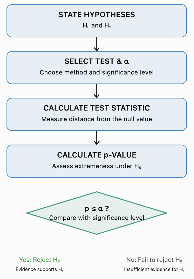
A hypothesis test generally involves five main steps:
-
State the null and alternative hypotheses.
-
Select an appropriate statistical test.
-
Calculate a test statistic.
-
Determine and interpret the p-value.
-
Make a statistical decision and explain the conclusion in context.
A successful hypothesis test requires both accurate calculations and careful interpretation. Statistical evidence is not the same as absolute proof.
What Is a Statistical Hypothesis?
A statistical hypothesis is a statement about a population parameter or probability distribution.
Common population parameters include:
-
μ: population mean.
-
p: population proportion.
-
μ₁ − μ₂: difference between two population means.
-
p₁ − p₂: difference between two population proportions.
Hypothesis testing uses sample statistics to evaluate these population claims.
For example, a school may want to determine whether the population mean test score is different from 70 marks.
The school collects a sample of test scores and evaluates whether the observed sample mean provides sufficient evidence of a difference.
The Null Hypothesis
The null hypothesis, written H₀, is the statement being tested.
In introductory tests, it commonly represents:
-
No change.
-
No difference.
-
No effect.
-
A specified population value.
Examples:
H₀: μ = 70
H₀: p = 0.50
H₀: μ₁ − μ₂ = 0
H₀: p₁ − p₂ = 0
The null hypothesis provides the reference model used to calculate how unusual the observed data would be.
The Alternative Hypothesis
The alternative hypothesis, written H₁ or Hₐ, describes the claim for which we seek evidence against H₀.
It may represent:
-
An increase.
-
A decrease.
-
A difference.
-
A nonzero effect.
Examples:
H₁: μ > 70
H₁: μ < 70
H₁: μ ≠ 70
The alternative hypothesis determines whether the test is one-tailed or two-tailed.
One-Tailed and Two-Tailed Tests
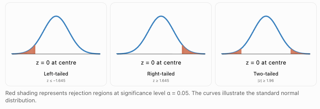
Right-Tailed Test
A right-tailed test investigates whether a population parameter is greater than a specified value.
Example:
H₀: μ = 100
H₁: μ > 100
This test looks for unusually large sample results.
Left-Tailed Test
A left-tailed test investigates whether a population parameter is less than a specified value.
Example:
H₀: μ = 100
H₁: μ < 100
This test looks for unusually small sample results.
Two-Tailed Test
A two-tailed test investigates whether a population parameter differs from a specified value in either direction.
Example:
H₀: μ = 100
H₁: μ ≠ 100
Both unusually large and unusually small results can provide evidence against H₀.
Rejection regions for three types of z-test
Worked Example 1: Formulating Hypotheses
A company claims that the average mass of a cereal packet is 500 g.
A consumer group suspects that the packets are underfilled.
Step 1: Identify the parameter
Let μ be the population mean mass of all packets produced.
Step 2: Write the null hypothesis
H₀: μ = 500 g.
Step 3: Write the alternative hypothesis
H₁: μ < 500 g.
Step 4: Identify the test direction
The alternative hypothesis uses the less-than symbol.
Therefore, this is a left-tailed test.
The consumer group is seeking evidence that the mean packet mass is below 500 g.
Worked Example 2: Choosing a Two-Tailed Test
A school introduces a new teaching method and wants to investigate whether the mean mathematics score differs from the historical mean of 75 marks.
The school is interested in either improvement or decline.
Let μ be the population mean score under the new method.
H₀: μ = 75.
H₁: μ ≠ 75.
Answer: A two-tailed test.
The direction must be selected from the research question before examining the sample results. Choosing the direction after seeing the data can invalidate the reported p-value.
The Logic of Hypothesis Testing
Hypothesis testing begins by temporarily assuming that H₀ is true.
We then ask:
If H₀ were true, how unusual would the observed sample result be?
If the result is very unusual under H₀, it provides evidence against H₀.
If the result is not sufficiently unusual, we do not have enough evidence to reject H₀.
This does not establish that H₀ is true.
The General Process
The Significance Level
The significance level, written α (alpha), is the threshold used to decide whether a result is statistically significant.
Common choices are:
|
Significance level |
Percentage |
|---|---|
|
α = 0.10 |
10% |
|
α = 0.05 |
5% |
|
α = 0.01 |
1% |
The significance level should be chosen before examining the results.
At α = 0.05:
-
If p ≤ 0.05, reject H₀.
-
If p > 0.05, fail to reject H₀.
The value α represents the maximum probability of a Type I error under the test's null model and assumptions.
A smaller α requires stronger evidence before rejecting H₀.
Calculating Test Statistics
A test statistic measures how far a sample result is from the value predicted by H₀, relative to the sampling variability expected under H₀.
A general structure is:
Test statistic = (Observed estimate − Null value) / Standard error
A large absolute test statistic indicates that the observed result is far from the null value relative to its standard error.
Different hypothesis tests use different test statistics.
z-Test for a Population Mean
When the population standard deviation σ is known, a one-sample z-test may be appropriate.
Formula:
z = (x̄ − μ₀)/(σ/√n)
Where:
-
x̄ = sample mean.
-
μ₀ = population mean specified by H₀.
-
σ = known population standard deviation.
-
n = sample size.
The test assumes an appropriate random and independent sampling process and a normal or approximately normal sampling distribution of the mean.
Worked Example 3: Calculating a z-Test Statistic
A factory claims that the mean lifetime of its batteries is 500 hours.
A random sample of 64 batteries has:
x̄ = 485 hours.
σ = 40 hours.
Test whether the population mean is less than 500 hours.
Step 1: State the hypotheses
H₀: μ = 500.
H₁: μ < 500.
Step 2: Identify the information
x̄ = 485.
μ₀ = 500.
σ = 40.
n = 64.
Step 3: Calculate the standard error
SE = σ/√n
= 40/√64
= 40/8
= 5 hours.
Step 4: Calculate z
z = (485 − 500)/5
= −15/5
= −3.00.
Answer: z = −3.00.
The sample mean is three standard errors below the null-hypothesis mean.
A z-value of −3 is unusually low under the standard normal distribution.
The Standard Normal Distribution
Under H₀ and the z-test assumptions, the z-statistic follows a standard normal distribution, exactly or approximately.
The standard normal distribution has:
Mean = 0.
Standard deviation = 1.
Its shape is symmetric and bell-shaped.
Values close to zero are common, while values far from zero are less common.
The p-value is calculated from the appropriate tail area or areas of this distribution.
Understanding p-Values
The p-value is the probability, assuming the null hypothesis and the statistical model are correct, of obtaining a test statistic at least as extreme as the one observed, in the direction or directions specified by the alternative hypothesis.
A small p-value means that the observed result would be relatively unusual under H₀.
A large p-value means that the result is not particularly unusual under H₀.
Importantly:
-
A p-value is not the probability that H₀ is true.
-
A p-value is not the probability that the results occurred purely by chance.
-
A small p-value does not measure the size or practical importance of an effect.
-
A large p-value does not prove that H₀ is true.
Calculating p-Values from z-Statistics
Let Φ(z) represent the cumulative probability to the left of z under the standard normal distribution.
|
Alternative hypothesis |
p-value |
|---|---|
|
H₁: μ < μ₀ |
Φ(z) |
|
H₁: μ > μ₀ |
1 − Φ(z) |
|
H₁: μ ≠ μ₀ |
2Φ(−|z|) |
For a two-tailed test, the probability is calculated using both tails.
Worked Example 4: Completing the Battery Hypothesis Test
Return to the battery investigation.
H₀: μ = 500 hours.
H₁: μ < 500 hours.
Calculated test statistic:
z = −3.00.
Use α = 0.05.
Step 1: Calculate the p-value
Because this is a left-tailed test:
p = P(Z ≤ −3.00)
≈ 0.00135.
Step 2: Compare with α
0.00135 < 0.05.
Therefore, reject H₀.
Step 3: State the conclusion
There is statistically significant evidence at the 5% significance level that the population mean battery lifetime is less than 500 hours.
Step 4: Interpret the p-value
If the population mean really were 500 hours and the model assumptions held, the probability of obtaining a sample mean of 485 hours or less from a sample of 64 batteries would be approximately 0.135%.
This is strong evidence against the manufacturer's claimed mean.
It does not prove that every battery lasts less than 500 hours.
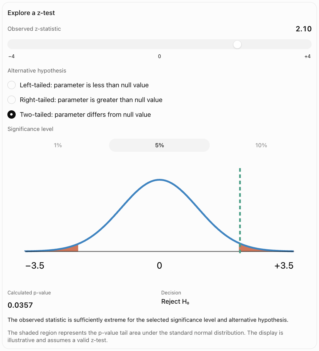
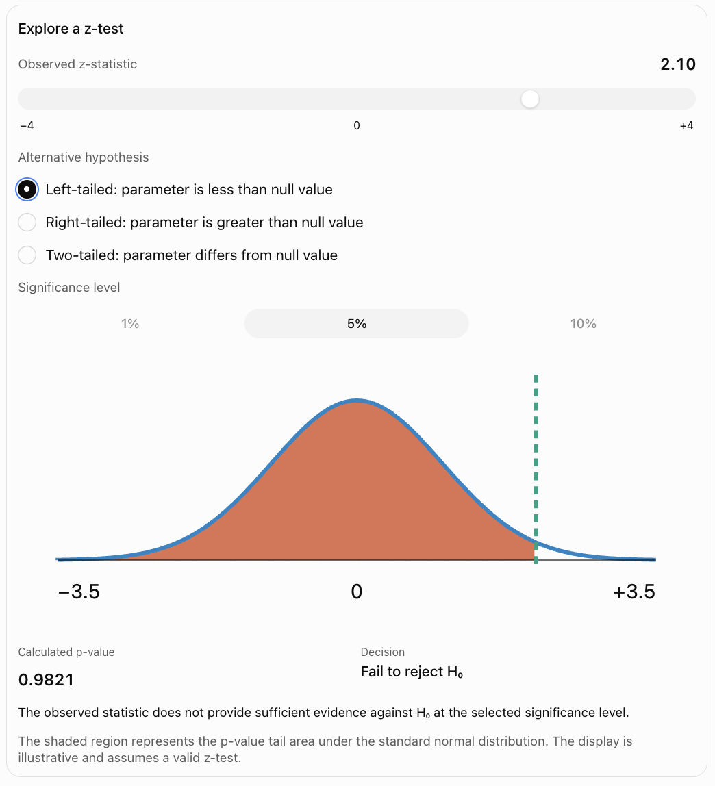
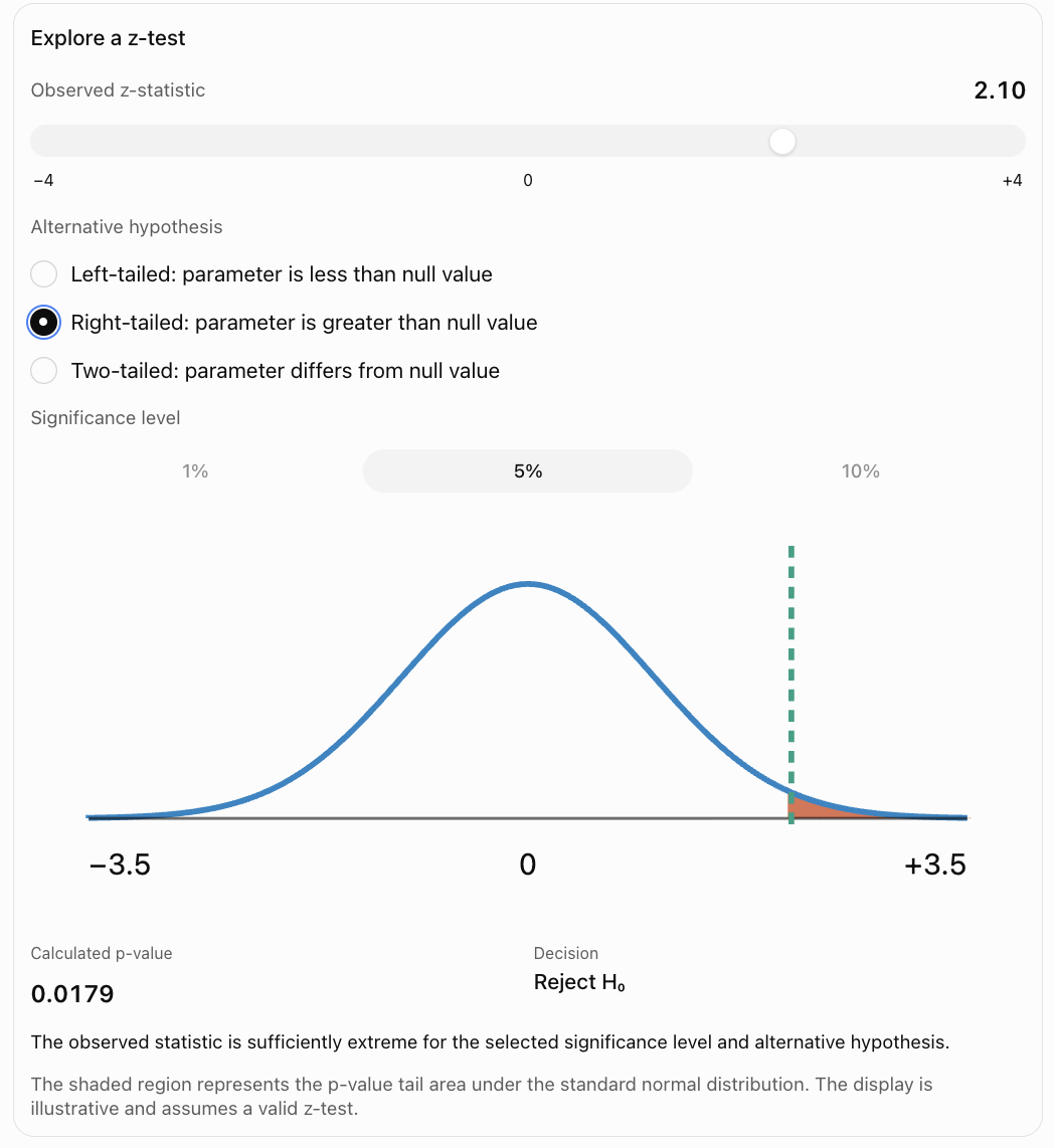
Interactive Hypothesis-Test Explorer
Use the controls to explore how the test statistic, alternative hypothesis, and significance level affect the statistical decision.
Worked Example 5: A Right-Tailed z-Test
A company claims that the mean delivery time is 30 minutes.
A random sample of 100 deliveries gives:
x̄ = 32.4 minutes.
The known population standard deviation is:
σ = 10 minutes.
Test whether the mean delivery time exceeds 30 minutes at α = 0.05.
Step 1: Hypotheses
H₀: μ = 30.
H₁: μ > 30.
Step 2: Standard error
SE = 10/√100 = 1.
Step 3: Test statistic
z = (32.4 − 30)/1
= 2.40.
Step 4: p-value
p = P(Z ≥ 2.40)
≈ 0.0082.
Step 5: Decision
0.0082 < 0.05.
Reject H₀.
Conclusion: There is statistically significant evidence that the population mean delivery time exceeds 30 minutes.
The sample mean suggests an increase of 2.4 minutes. Whether this increase is practically important depends on the business context.
Worked Example 6: A Two-Tailed z-Test
A filling machine is designed to dispense a mean of 250 mL.
A sample of 64 containers has:
x̄ = 247 mL.
σ = 12 mL.
Test whether the mean filling volume differs from 250 mL at α = 0.05.
Step 1: Hypotheses
H₀: μ = 250.
H₁: μ ≠ 250.
Step 2: Standard error
SE = 12/√64
= 1.5 mL.
Step 3: Test statistic
z = (247 − 250)/1.5
= −2.00.
Step 4: Two-tailed p-value
p = 2P(Z ≤ −2.00)
≈ 2(0.02275)
≈ 0.0455.
Step 5: Decision
0.0455 < 0.05.
Reject H₀.
Conclusion: There is statistically significant evidence that the population mean filling volume differs from 250 mL.
The sample indicates that the mean may be lower than the target.
Because this was a two-tailed test, the p-value includes extreme results in both directions.
t-Tests for a Population Mean
In many investigations, the population standard deviation σ is unknown.
Instead, the sample standard deviation s is used.
For a one-sample mean test, the appropriate statistic is usually:
t = (x̄ − μ₀)/(s/√n)
The degrees of freedom are:
df = n − 1
The p-value is calculated using Student's t-distribution.
A t-test requires an appropriate sampling design and distributional conditions. For small samples, the observations should be approximately normally distributed without severe outliers; larger samples allow more flexibility.
Worked Example 7: One-Sample t-Test
A school believes that the population mean mathematics test score is 70 marks.
A random sample of 25 students produces:
x̄ = 74.
s = 10.
Test whether the population mean score is different from 70 at α = 0.05.
Assume the t-test conditions hold.
Step 1: Hypotheses
H₀: μ = 70.
H₁: μ ≠ 70.
Step 2: Degrees of freedom
df = 25 − 1 = 24.
Step 3: Standard error
SE = 10/√25
= 2.
Step 4: Test statistic
t = (74 − 70)/2
= 2.00.
Step 5: p-value
For t = 2.00 with 24 degrees of freedom, using a two-tailed test:
p ≈ 0.057.
Step 6: Decision
0.057 > 0.05.
Fail to reject H₀.
Conclusion: There is insufficient statistical evidence at the 5% significance level that the population mean mathematics score differs from 70 marks.
This does not prove that the population mean is exactly 70.
The result is close to the significance threshold, illustrating why reporting the actual p-value is more informative than reporting only the decision.
Worked Example 8: A Left-Tailed t-Test
A factory claims that its components have a mean breaking strength of 100 N.
A random sample of 16 components has:
x̄ = 94 N.
s = 12 N.
Test whether the population mean breaking strength is less than 100 N.
Assume the population distribution is approximately normal.
Use α = 0.05.
Step 1: Hypotheses
H₀: μ = 100.
H₁: μ < 100.
Step 2: Degrees of freedom
df = 15.
Step 3: Standard error
SE = 12/√16 = 3 N.
Step 4: Test statistic
t = (94 − 100)/3
= −2.00.
Step 5: p-value
For t = −2.00 with df = 15, left-tailed:
p ≈ 0.032.
Step 6: Decision
0.032 < 0.05.
Reject H₀.
Conclusion: There is statistically significant evidence that the population mean breaking strength is below 100 N.
This may justify further quality-control investigation.
Hypothesis Tests for Population Proportions
Hypothesis tests are also used to investigate population proportions.
Examples include the proportion of students who prefer a new timetable, the percentage of defective products, and the proportion of households using renewable energy.
The sample proportion is:
p̂ = x/n
Where x is the number of observations with the characteristic and n is the sample size.
For a one-sample proportion z-test:
z = (p̂ − p₀)/√(p₀(1 − p₀)/n)
Where p₀ is the population proportion specified by H₀.
Notice that the standard error uses p₀, not p̂. This is because the test statistic is calculated under the null hypothesis.
For the normal approximation, common conditions include:
n p₀ ≥ 10
and
n(1 − p₀) ≥ 10.
The observations should also be independent or approximately independent, and the sampling design should be appropriate.
Worked Example 9: Testing a Population Proportion
A school claims that 50% of students prefer digital textbooks.
A random sample of 200 students finds that 120 prefer digital textbooks.
Test whether the population proportion is greater than 50% at α = 0.05.
Step 1: Hypotheses
H₀: p = 0.50.
H₁: p > 0.50.
Step 2: Calculate the sample proportion
p̂ = 120/200
= 0.60.
Step 3: Check the approximation
n p₀ = 200 × 0.50 = 100.
n(1 − p₀) = 100.
Both exceed 10.
Step 4: Calculate standard error under H₀
SE₀ = √(0.50 × 0.50/200)
= √0.00125
≈ 0.03536.
Step 5: Calculate the test statistic
z = (0.60 − 0.50)/0.03536
≈ 2.83.
Step 6: Calculate the p-value
This is a right-tailed test.
p = P(Z ≥ 2.83)
≈ 0.0023.
Step 7: Decision
0.0023 < 0.05.
Reject H₀.
Conclusion: There is statistically significant evidence that more than 50% of students in the population prefer digital textbooks.
Worked Example 10: Testing a Defect Rate
A manufacturer claims that 5% of its products are defective.
A random sample of 400 products contains 30 defective items.
Test whether the population defect rate exceeds 5% at α = 0.05.
Step 1: Hypotheses
H₀: p = 0.05.
H₁: p > 0.05.
Step 2: Sample proportion
p̂ = 30/400
= 0.075.
Step 3: Check conditions
n p₀ = 400 × 0.05 = 20.
n(1 − p₀) = 380.
The normal approximation is reasonable.
Step 4: Standard error
SE₀ = √(0.05 × 0.95/400)
≈ 0.01090.
Step 5: Test statistic
z = (0.075 − 0.05)/0.01090
≈ 2.29.
Step 6: p-value
p ≈ 0.0109.
Step 7: Decision
0.0109 < 0.05.
Reject H₀.
Conclusion: There is statistically significant evidence that the population defect rate exceeds 5%.
This finding could motivate further inspection of the manufacturing process.
Making Statistical Decisions
Once the p-value has been calculated, compare it with the chosen significance level.
|
Comparison |
Decision |
Meaning |
|---|---|---|
|
p ≤ α |
Reject H₀ |
Sufficient statistical evidence against H₀ |
|
p > α |
Fail to reject H₀ |
Insufficient statistical evidence against H₀ |
We generally avoid saying accept H₀.
A failure to reject may occur because the null hypothesis is correct, because the sample is too small, or because the true effect is difficult to detect.
Worked Example 11: Different Significance Levels
A hypothesis test produces:
p = 0.032.
Determine the decision at three significance levels.
|
Significance level |
Comparison |
Decision |
|---|---|---|
|
α = 0.10 |
0.032 < 0.10 |
Reject H₀ |
|
α = 0.05 |
0.032 < 0.05 |
Reject H₀ |
|
α = 0.01 |
0.032 > 0.01 |
Fail to reject H₀ |
The data and p-value have not changed.
Only the decision threshold has changed.
This demonstrates why a statistical report should include the p-value and the chosen significance level rather than simply stating that a result is significant.
Type I and Type II Errors
Hypothesis testing involves the possibility of incorrect decisions.
Type I Error
A Type I error occurs when H₀ is rejected even though it is true.
This is sometimes called a false positive.
The probability of a Type I error is controlled by the significance level α, under the test assumptions.
Type II Error
A Type II error occurs when H₀ is not rejected even though a particular alternative is true.
This is sometimes called a false negative.
The probability of a Type II error is represented by β (beta), for a specified alternative.
|
Reality |
Reject H₀ |
Fail to reject H₀ |
|---|---|---|
|
H₀ is true |
Type I error |
Correct decision |
|
H₀ is false |
Correct rejection |
Type II error |
Statistical Power
The power of a test is the probability of rejecting H₀ when a specified alternative is true.
Power = 1 − β
Higher power means a greater chance of detecting a real effect of the specified size.
Power is affected by:
-
Sample size.
-
Effect size.
-
Population variability.
-
Significance level.
-
Choice of statistical test.
Larger samples generally increase power when other conditions remain unchanged.
Worked Example 12: Understanding Errors in Context
A company tests whether its mean product mass is below the advertised 500 g.
H₀: μ = 500.
H₁: μ < 500.
A Type I error would occur if the company concluded that the population mean was below 500 g when the null value of 500 g was actually correct.
A Type II error would occur if the company failed to detect an actual reduction in mean mass.
The consequences differ.
A Type I error could cause unnecessary investigations or production changes.
A Type II error could allow an underfilling problem to continue.
The appropriate significance level should reflect the consequences of these errors, not merely a conventional choice of 0.05.
Statistical Significance Versus Practical Significance
A statistically significant result is not necessarily important in real life.
Suppose a very large sample finds that a new teaching method increases the mean test score by 0.2 marks.
The result might have a very small p-value because the estimate is extremely precise.
However, an increase of only 0.2 marks may have little practical educational value.
Conversely, a small study might estimate a substantial improvement but fail to reach statistical significance because the estimate is too uncertain.
Worked Example 13: A Large Sample with a Small Effect
A process has a historical mean output of 100 units.
A sample of 10,000 observations produces:
x̄ = 100.5.
Known σ = 10.
Test:
H₀: μ = 100.
H₁: μ ≠ 100.
Step 1: Standard error
SE = 10/√10000
= 0.1.
Step 2: Test statistic
z = (100.5 − 100)/0.1
= 5.00.
Step 3: p-value
The two-tailed p-value is approximately:
p ≈ 0.00000057.
This is statistically significant at α = 0.05.
However, the estimated increase is only 0.5 units, or 0.5% of the historical mean.
Conclusion: The data provide strong statistical evidence of a difference, but the practical importance of that difference must be evaluated separately.
Connecting Hypothesis Tests and Confidence Intervals
Hypothesis testing and confidence intervals are closely related.
For many standard two-sided tests, a hypothesis test at significance level α corresponds to a confidence interval with confidence level:
100(1 − α)%
For example:
A two-sided test at α = 0.05 corresponds to a 95% confidence interval when the test and interval use matching methods and assumptions.
If the null-hypothesis value lies outside the confidence interval, reject H₀.
If the null-hypothesis value lies inside the interval, fail to reject H₀.
This correspondence applies to compatible two-sided procedures; it should not be applied indiscriminately to one-sided tests or intervals constructed using different methods.
Worked Example 14: Testing with a Confidence Interval
A sample gives:
x̄ = 52.
Known σ = 12.
n = 36.
Test:
H₀: μ = 48.
H₁: μ ≠ 48.
Use α = 0.05.
Step 1: Calculate the standard error
SE = 12/√36
= 2.
Step 2: Construct the 95% confidence interval
CI = 52 ± 1.96 × 2
= 52 ± 3.92.
CI = (48.08, 55.92).
Step 3: Compare the null value
The null value is 48.
Since 48 lies outside the interval, reject H₀.
Step 4: Check with a test statistic
z = (52 − 48)/2
= 2.00.
Two-tailed p ≈ 0.0455.
Since p < 0.05, reject H₀.
Conclusion: Both methods agree that there is statistically significant evidence that the population mean differs from 48.
The confidence interval also provides a range of plausible values for the population mean, making it especially useful for communicating the size and uncertainty of the estimated effect.
Choosing the Appropriate Hypothesis Test
The correct test depends on the type of data, the parameter being investigated, and the study design.
|
Research question |
Common statistical test |
|---|---|
|
Is a population mean different from a specified value, with σ known? |
One-sample z-test |
|
Is a population mean different from a specified value, with σ unknown? |
One-sample t-test |
|
Is a population proportion different from a specified value? |
One-proportion z-test |
|
Do two independent population means differ? |
Two-sample t-test |
|
Is the mean difference between paired measurements zero? |
Paired t-test |
|
Do two population proportions differ? |
Two-proportion z-test |
|
Are two categorical variables associated? |
Chi-square test of independence |
Each test has assumptions that must be checked.
For example, a paired t-test is appropriate when the same students are measured before and after an intervention, while a two-sample t-test may be appropriate when comparing independent groups of students.
Worked Example 15: Paired Data
Ten students complete a mathematics assessment before and after a teaching intervention.
For each student, calculate:
Difference = After score − Before score.
The ten differences have:
Mean difference d̄ = 4.5 marks.
Standard deviation of differences s_d = 5 marks.
Test whether the mean improvement is greater than zero.
Assume the differences are approximately normally distributed and students are independently sampled.
Step 1: Hypotheses
Let μ_d be the population mean score difference.
H₀: μ_d = 0.
H₁: μ_d > 0.
Step 2: Standard error
SE = s_d/√n
= 5/√10
≈ 1.581.
Step 3: Test statistic
t = 4.5/1.581
≈ 2.846.
Step 4: Degrees of freedom
df = 10 − 1 = 9.
Step 5: p-value
For a right-tailed test:
p ≈ 0.0096.
Step 6: Decision
0.0096 < 0.05.
Reject H₀.
Conclusion: There is statistically significant evidence that the population mean after-minus-before score difference is positive.
However, without an appropriate comparison group, the improvement cannot automatically be attributed entirely to the teaching intervention. Other influences may have affected the scores.
Communicating the Conclusions of Hypothesis Tests
A complete statistical conclusion should contain four elements:
-
The statistical decision.
-
The significance level.
-
The population parameter and direction of the claim.
-
The strength and limitations of the evidence.
Example: Rejecting H₀
"At the 5% significance level, the test provides statistically significant evidence that the population mean battery lifetime is less than 500 hours (z = −3.00, p ≈ 0.00135)."
Example: Failing to Reject H₀
"At the 5% significance level, there is insufficient statistical evidence that the population mean test score differs from 70 marks (t = 2.00, df = 24, p ≈ 0.057)."
Avoid These Statements
Incorrect: "The null hypothesis is definitely false."
A hypothesis test provides evidence, not certainty.
Incorrect: "The null hypothesis is true because p > 0.05."
Failure to reject H₀ does not establish that H₀ is true.
Incorrect: "There is a 3% chance that the null hypothesis is true."
A p-value of 0.03 does not represent the probability that H₀ is true.
Incorrect: "The result is important because p < 0.05."
Statistical significance does not automatically establish practical importance.
Evaluating the Reliability of a Hypothesis Test
Before accepting a statistical conclusion, consider:
Sampling: Was the sample randomly selected and representative?
Independence: Are the observations independent, or was dependence properly modelled?
Distribution: Are the assumptions of the selected test reasonable?
Sample size: Is the sample large enough to provide useful power and support any approximations?
Measurement: Were the data collected accurately?
Effect size: How large is the observed difference?
Multiple testing: Were many hypotheses tested, increasing the chance of false positives?
Study design: Does the study support a causal conclusion, or only an association?
A small p-value cannot compensate for a fundamentally flawed study design.
Real-World Applications
Scientific research
Researchers test whether experimental results provide evidence of changes, differences, or relationships.
Quality control
Manufacturers test whether production processes meet target values and defect-rate requirements.
Education
Schools investigate whether student achievement differs from benchmarks or changes after interventions.
Environmental science
Scientists test claims about pollution levels, environmental changes, and water quality.
Integrated Investigation: Does a New Study Programme Improve Results?
A school introduces an optional mathematics study programme.
Historically, the mean score on a standardized assessment is 70 marks.
A random sample of 36 participating students obtains:
x̄ = 75 marks.
s = 12 marks.
The school wants to determine whether the population mean score among programme participants exceeds 70 marks.
Assume the observations are independent and the t-test conditions are appropriate.
Step 1: State the Hypotheses
H₀: μ = 70.
H₁: μ > 70.
Step 2: Select the Test
The population standard deviation is unknown.
Therefore, use a one-sample t-test.
Step 3: Choose the Significance Level
α = 0.05.
Step 4: Calculate the Standard Error
SE = 12/√36
= 2 marks.
Step 5: Calculate the Test Statistic
t = (75 − 70)/2
= 2.50.
Step 6: Degrees of Freedom
df = 36 − 1 = 35.
Step 7: Calculate the p-Value
For t = 2.50, df = 35, right-tailed:
p ≈ 0.0086.
Step 8: Make the Decision
0.0086 < 0.05.
Reject H₀.
Step 9: Communicate the Conclusion
There is statistically significant evidence at the 5% significance level that the population mean score among students participating in the programme exceeds 70 marks.
Step 10: Evaluate the Investigation
This does not prove that the programme caused the higher scores.
Students who volunteered for the programme may already be more motivated or better prepared.
A stronger causal investigation would use random assignment to programme and comparison groups, with appropriate analysis of the resulting outcomes.
This example demonstrates how hypothesis testing combines mathematical calculation, statistical interpretation, and critical evaluation.
Common Mistakes
Mistake 1: Confusing H₀ and H₁
The null hypothesis specifies the reference claim. The alternative describes the effect or difference being investigated.
Mistake 2: Using Sample Statistics in Hypotheses
Hypotheses concern population parameters, such as μ or p, rather than observed sample values such as x̄ or p̂.
Mistake 3: Choosing the Test Direction After Seeing the Data
The alternative hypothesis should be determined from the research question before examining the results.
Mistake 4: Using a Two-Tailed p-Value for a One-Tailed Test
The p-value must correspond to the specified alternative hypothesis.
Mistake 5: Forgetting the Standard Error
A test statistic compares a difference with its expected sampling variability, not merely with the raw standard deviation.
Mistake 6: Using σ When It Is Unknown
For a one-sample mean test with unknown σ, the t-test is generally appropriate.
Mistake 7: Forgetting Degrees of Freedom
For a one-sample t-test, df = n − 1.
Mistake 8: Using p̂ Instead of p₀ in a One-Proportion z-Test Standard Error
The test statistic uses the standard error calculated under H₀.
Mistake 9: Misinterpreting the p-Value
The p-value is not the probability that H₀ is true.
Mistake 10: Saying "Accept H₀"
The standard conclusion is "fail to reject H₀" when the evidence is insufficient.
Mistake 11: Treating Statistical Significance as Proof
Even statistically significant findings can be affected by sampling error, bias, or incorrect assumptions.
Mistake 12: Confusing Statistical Significance with Practical Importance
A very small effect may be statistically significant in a large sample.
Mistake 13: Ignoring Type I and Type II Errors
Both false rejection and failure to detect a real effect have consequences.
Mistake 14: Ignoring Sampling Bias
A large biased sample does not automatically support valid population inference.
Mistake 15: Failing to Check Test Assumptions
Independence, distributional conditions, and sampling design matter.
Mistake 16: Assuming a Nonsignificant Result Proves No Effect
The test may have insufficient power to detect a real effect.
Mistake 17: Using Inappropriate Precision
Report calculated values to a sensible number of decimal places without rounding intermediate calculations excessively.
Mistake 18: Making a Causal Claim from an Observational Study
An association or statistically significant difference does not necessarily establish causation.
Mistake 19: Ignoring Multiple Comparisons
Testing many hypotheses without appropriate adjustment increases the chance of obtaining false-positive findings.
Mistake 20: Giving a Decision Without Context
A complete conclusion should explain what the evidence means for the population and research question.
Key Terms
-
Hypothesis Testing: A statistical procedure for evaluating a claim about a population.
-
Statistical Hypothesis: A statement about a population parameter or distribution.
-
Null Hypothesis (H₀): The reference hypothesis evaluated by a statistical test.
-
Alternative Hypothesis (H₁ or Hₐ): The competing claim for which evidence is sought.
-
Population Parameter: A numerical characteristic of a population.
-
Sample Statistic: A numerical characteristic calculated from sample data.
-
Test Statistic: A standardized or otherwise defined measure of evidence against H₀.
-
z-Test: A test using the standard normal distribution under appropriate assumptions.
-
t-Test: A test using Student's t-distribution.
-
One-Tailed Test: A test for an effect in a specified direction.
-
Left-Tailed Test: A test with a less-than alternative.
-
Right-Tailed Test: A test with a greater-than alternative.
-
Two-Tailed Test: A test for a difference in either direction.
-
Significance Level (α): The chosen threshold controlling the Type I error probability.
-
p-Value: The probability under H₀ of a test statistic at least as extreme as the observed one.
-
Statistical Significance: A result meeting the chosen criterion for rejecting H₀.
-
Standard Error: The standard deviation of a statistic's sampling distribution, or an estimate of it.
-
Critical Value: A cutoff defining a rejection region.
-
Rejection Region: Values of a test statistic that lead to rejection of H₀.
-
Degrees of Freedom: A parameter determining the relevant t-distribution.
-
Type I Error: Rejecting a true null hypothesis.
-
Type II Error: Failing to reject a false null hypothesis.
-
Statistical Power: The probability of rejecting H₀ under a specified alternative.
-
Effect Size: A measure of the magnitude of an effect or difference.
-
Practical Significance: The real-world importance of an effect.
-
Confidence Interval: An interval estimate with a specified long-run coverage rate.
-
Sampling Variability: Differences between statistics obtained from different samples.
-
Random Sampling: Selecting observations using a chance-based procedure.
-
Sampling Bias: Systematic distortion caused by an unrepresentative selection process.
-
Normal Approximation: Using a normal distribution to approximate a sampling distribution.
-
Paired t-Test: A t-test applied to differences between paired observations.
-
Two-Sample t-Test: A test comparing the means of two independent populations.
-
One-Proportion z-Test: A test evaluating a population proportion using a normal approximation.
-
Multiple Testing: Conducting several hypothesis tests, potentially increasing false-positive risk.
-
Statistical Inference: Drawing conclusions about populations using sample data.
Key Takeaways
-
Hypothesis testing evaluates claims about population parameters.
-
The null hypothesis provides the reference model.
-
The alternative hypothesis specifies the claim being investigated.
-
Tests may be left-tailed, right-tailed, or two-tailed.
-
The test direction should be selected before examining the data.
-
A test statistic measures the observed difference relative to sampling variability.
-
z-tests and t-tests are used under different conditions.
-
One-proportion z-tests use the null proportion when calculating standard error.
-
A p-value measures how extreme the observed statistic is under H₀.
-
A small p-value provides evidence against H₀.
-
The significance level establishes the rejection threshold.
-
When p ≤ α, reject H₀.
-
When p > α, fail to reject H₀.
-
Failing to reject H₀ does not prove H₀ true.
-
Type I errors involve rejecting true null hypotheses.
-
Type II errors involve failing to detect false null hypotheses.
-
Statistical power describes the probability of detecting a specified real effect.
-
Statistical significance and practical significance are different.
-
Confidence intervals and compatible two-sided hypothesis tests are closely connected.
-
A complete conclusion includes the decision, evidence, context, and limitations.
Check Your Understanding
Use α = 0.05 unless another significance level is stated. Show your calculations and explain your decisions in context.
Question 1: Formulating Hypotheses
A company claims that the mean mass of its cereal packets is 400 g.
A researcher suspects that the mean mass is lower.
State H₀ and H₁, and identify the test direction.
Question 2: Two-Tailed Hypotheses
A school wants to investigate whether its population mean mathematics score differs from 75 marks.
Write the hypotheses and explain why the test is two-tailed.
Question 3: Calculating a z-Statistic
A sample of 100 measurements has:
x̄ = 54.
μ₀ = 50.
σ = 20.
Calculate the z-test statistic.
Question 4: Left-Tailed z-Test
A random sample of 64 products has:
x̄ = 98 g.
μ₀ = 100 g.
σ = 8 g.
Test whether the population mean mass is below 100 g.
Use the standard normal distribution.
Question 5: Right-Tailed z-Test
A sample of 100 observations has:
x̄ = 105.
μ₀ = 100.
σ = 20.
Test whether the population mean exceeds 100.
Question 6: Interpreting a p-Value
A hypothesis test produces p = 0.018.
Explain what the p-value means and state the decision at α = 0.05.
Question 7: Different Significance Levels
A test produces p = 0.034.
Determine the decision at:
a) α = 0.10.
b) α = 0.05.
c) α = 0.01.
Question 8: One-Sample t-Test
A random sample of 16 students has:
x̄ = 78.
s = 8.
Test whether the population mean score exceeds 75.
Assume the t-test conditions hold.
Use the t-distribution with 15 degrees of freedom.
Question 9: Population Proportion
A random sample of 200 students finds that 130 prefer digital learning materials.
Test whether the population proportion exceeds 0.50.
Question 10: Defect Rate
A manufacturer claims that 10% of its products are defective.
A random sample of 300 products contains 42 defective products.
Test whether the population defect proportion exceeds 10%.
Question 11: Type I and Type II Errors
A researcher tests whether the population mean concentration of a pollutant exceeds a specified safety threshold.
Explain Type I and Type II errors in this context.
Question 12: Statistical Versus Practical Significance
A large study finds that a new educational intervention increases average test scores by 0.1 marks, with p = 0.001.
Explain the statistical conclusion and why the result may not be practically important.
Question 13: Confidence Interval Connection
A 95% confidence interval for a population mean is:
(48, 56).
For a compatible two-sided test at α = 0.05, determine whether to reject H₀ when:
a) μ₀ = 50.
b) μ₀ = 45.
Question 14: Identifying Flawed Reasoning
A student writes:
"Because p = 0.12, there is a 12% probability that the null hypothesis is true. Therefore, we should accept the null hypothesis."
Identify and correct the errors.
Question 15: Comprehensive Hypothesis Test
A school claims that the population mean time students spend completing a mathematics assessment is 60 minutes.
A random sample of 36 students gives:
x̄ = 64 minutes.
s = 12 minutes.
Assume the t-test conditions hold.
Test whether the population mean completion time differs from 60 minutes.
Use:
α = 0.05.
For 35 degrees of freedom, the two-tailed p-value for t = 2.00 is approximately 0.053.
Calculate and explain:
a) The hypotheses.
b) The appropriate test.
c) The standard error.
d) The test statistic.
e) The p-value.
f) The statistical decision.
g) The conclusion in context.
h) Two limitations of the investigation.
Fully Worked Answers
Answer 1: Formulating Hypotheses
Let μ be the population mean mass of cereal packets.
H₀: μ = 400 g.
H₁: μ < 400 g.
Answer: Left-tailed test, because the researcher suspects that the mean is below 400 g.
Answer 2: Two-Tailed Hypotheses
Let μ be the population mean mathematics score.
H₀: μ = 75.
H₁: μ ≠ 75.
Answer: Two-tailed test.
The school is interested in differences in either direction, not only higher or lower scores.
Answer 3: Calculating a z-Statistic
Given:
x̄ = 54.
μ₀ = 50.
σ = 20.
n = 100.
Step 1: Standard error
SE = 20/√100
= 2.
Step 2: z-statistic
z = (54 − 50)/2
= 2.00.
Answer: z = 2.00.
The sample mean is two standard errors above the null value.
Answer 4: Left-Tailed z-Test
Step 1: Hypotheses
H₀: μ = 100.
H₁: μ < 100.
Step 2: Standard error
SE = 8/√64
= 1 g.
Step 3: Test statistic
z = (98 − 100)/1
= −2.00.
Step 4: p-value
p = P(Z ≤ −2.00)
≈ 0.0228.
Step 5: Decision
0.0228 < 0.05.
Reject H₀.
Conclusion: There is statistically significant evidence that the population mean product mass is below 100 g.
Answer 5: Right-Tailed z-Test
Step 1: Hypotheses
H₀: μ = 100.
H₁: μ > 100.
Step 2: Standard error
SE = 20/√100
= 2.
Step 3: Test statistic
z = (105 − 100)/2
= 2.50.
Step 4: p-value
p = P(Z ≥ 2.50)
≈ 0.0062.
Step 5: Decision
0.0062 < 0.05.
Reject H₀.
Conclusion: There is statistically significant evidence that the population mean exceeds 100.
Answer 6: Interpreting a p-Value
p = 0.018.
This means that, assuming H₀ and the statistical model are correct, the probability of obtaining a test statistic at least as extreme as the observed one is 1.8%, in the direction or directions specified by H₁.
Since:
0.018 < 0.05,
reject H₀.
Answer: The result is statistically significant at the 5% level.
Answer 7: Different Significance Levels
p = 0.034.
a) α = 0.10
0.034 < 0.10.
Reject H₀.
b) α = 0.05
0.034 < 0.05.
Reject H₀.
c) α = 0.01
0.034 > 0.01.
Fail to reject H₀.
Conclusion: The decision depends on the significance threshold, even though the sample evidence remains unchanged.
Answer 8: One-Sample t-Test
Given:
x̄ = 78.
μ₀ = 75.
s = 8.
n = 16.
Step 1: Hypotheses
H₀: μ = 75.
H₁: μ > 75.
Step 2: Standard error
SE = 8/√16
= 2.
Step 3: Test statistic
t = (78 − 75)/2
= 1.50.
Step 4: Degrees of freedom
df = 15.
Step 5: p-value
For t = 1.50, df = 15, right-tailed:
p ≈ 0.077.
Step 6: Decision
0.077 > 0.05.
Fail to reject H₀.
Conclusion: There is insufficient statistical evidence that the population mean score exceeds 75 marks.
Answer 9: Population Proportion
Given:
x = 130.
n = 200.
Step 1: Hypotheses
H₀: p = 0.50.
H₁: p > 0.50.
Step 2: Sample proportion
p̂ = 130/200
= 0.65.
Step 3: Standard error
SE₀ = √(0.50 × 0.50/200)
≈ 0.03536.
Step 4: Test statistic
z = (0.65 − 0.50)/0.03536
≈ 4.24.
Step 5: p-value
The right-tailed p-value is approximately 0.000011.
Step 6: Decision
p < 0.05.
Reject H₀.
Conclusion: There is strong statistical evidence that more than 50% of students in the population prefer digital learning materials.
Answer 10: Defect Rate
Given:
x = 42.
n = 300.
Step 1: Hypotheses
H₀: p = 0.10.
H₁: p > 0.10.
Step 2: Sample proportion
p̂ = 42/300
= 0.14.
Step 3: Check approximation
n p₀ = 30.
n(1 − p₀) = 270.
Both exceed 10.
Step 4: Standard error
SE₀ = √(0.10 × 0.90/300)
= √0.0003
≈ 0.01732.
Step 5: Test statistic
z = (0.14 − 0.10)/0.01732
≈ 2.31.
Step 6: p-value
Right-tailed p ≈ 0.0105.
Step 7: Decision
0.0105 < 0.05.
Reject H₀.
Conclusion: There is statistically significant evidence that the population defect rate exceeds 10%.
Answer 11: Type I and Type II Errors
Suppose the hypotheses are:
H₀: μ = the safety threshold.
H₁: μ > the safety threshold.
Type I error: Concluding that the population mean pollutant concentration exceeds the threshold when the null value is actually correct.
This could lead to unnecessary warnings or interventions.
Type II error: Failing to detect that the population mean pollutant concentration exceeds the threshold when it actually does.
This could allow a genuine environmental problem to remain undetected.
Both errors matter, but their consequences may differ substantially.
Answer 12: Statistical Versus Practical Significance
Given:
p = 0.001.
Since:
0.001 < 0.05,
the result is statistically significant.
There is evidence that the intervention changes the population mean score, assuming the test and study design are valid.
However, the estimated increase is only 0.1 marks.
This may be too small to produce a meaningful educational benefit.
Conclusion: Statistical significance does not necessarily imply practical significance.
Answer 13: Confidence Interval Connection
95% CI = (48, 56).
Use a compatible two-sided test at α = 0.05.
a) μ₀ = 50
50 lies inside the interval.
Therefore:
Fail to reject H₀.
b) μ₀ = 45
45 lies outside the interval.
Therefore:
Reject H₀.
This illustrates the relationship between compatible two-sided hypothesis tests and confidence intervals.
Answer 14: Identifying Flawed Reasoning
The student's statement contains two errors.
Error 1: A p-value of 0.12 does not mean that H₀ has a 12% probability of being true.
It means that, assuming H₀ and the statistical model are correct, the probability of obtaining a result at least as extreme as the observed one is 12%.
Error 2: The correct decision is not to "accept H₀."
At α = 0.05:
0.12 > 0.05.
Therefore:
Fail to reject H₀.
There is insufficient evidence against the null hypothesis, but this does not establish that it is true.
Answer 15: Comprehensive Hypothesis Test
Given:
x̄ = 64 minutes.
μ₀ = 60 minutes.
s = 12 minutes.
n = 36.
α = 0.05.
a) Hypotheses
H₀: μ = 60.
H₁: μ ≠ 60.
The test is two-tailed because the question asks whether the population mean differs from 60 minutes.
b) Appropriate test
Use a one-sample t-test because the population standard deviation is unknown.
c) Standard error
SE = s/√n
= 12/√36
= 12/6
= 2 minutes.
Answer: SE = 2 minutes.
d) Test statistic
t = (64 − 60)/2
= 2.00.
Answer: t = 2.00.
e) p-value
Degrees of freedom:
df = 36 − 1 = 35.
Given:
Two-tailed p ≈ 0.053.
f) Statistical decision
0.053 > 0.05.
Fail to reject H₀.
g) Conclusion in context
At the 5% significance level, there is insufficient statistical evidence that the population mean mathematics assessment completion time differs from 60 minutes.
The sample mean is 64 minutes, but the observed difference is not statistically significant at the chosen threshold.
This does not prove that the true mean is exactly 60 minutes.
h) Two limitations
-
The sample may not fully represent the school population, especially if some student groups are underrepresented.
-
Completion times may be affected by differences in assessment difficulty, testing conditions, or student preparation.
A larger, representative sample and consistent testing conditions could improve the investigation.
Final Course Connections
Hypothesis testing connects probability distributions, sampling variability, standard errors, confidence intervals, and statistical inference.
It provides a structured way to evaluate claims using evidence rather than relying on individual observations or assumptions.
The essential process is to formulate appropriate hypotheses, select a valid statistical test, calculate the test statistic and p-value, make a decision using the significance level, and communicate the conclusion in the context of the original question.
The most important distinction is that hypothesis testing evaluates the strength of statistical evidence; it does not establish absolute certainty.
This completes Hypothesis Testing, covering all five learning targets with 15 worked examples, explanatory diagrams, an interactive z-test explorer, real-world applications, common mistakes, key terms, key takeaways, and 15 practice questions with fully worked answers.