Solving Polynomial Equations

Introduction

Polynomial equations are among the most useful mathematical tools for describing and solving real-world problems. They appear in engineering, architecture, economics, physics, manufacturing, environmental science, and many other fields.

Whenever a quantity depends on another through a relationship involving powers such as x², x³, or x⁴, a polynomial model may be appropriate.

For example, a manufacturer may want to determine the dimensions of a box that produces a particular volume. An engineer may need to calculate when a moving object reaches a certain height. A business owner may use a polynomial revenue function to determine how many products must be sold to reach a financial target.

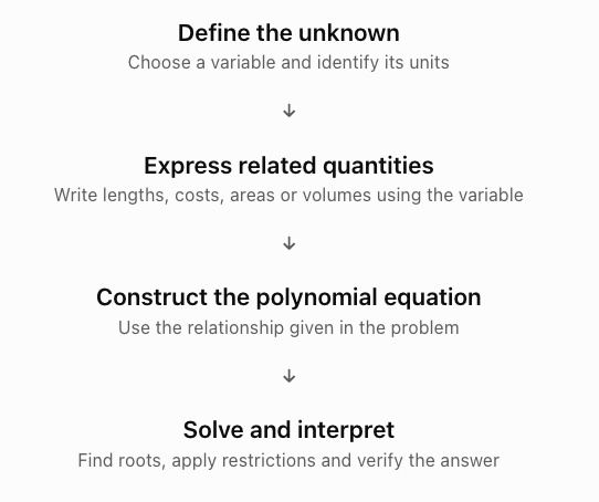
In each case, the mathematics follows a similar process: identify the variables, construct an equation, solve it, and interpret the solutions within the original situation.

However, finding the roots of a polynomial is only part of the problem. Some roots may be negative, outside the permitted domain, or otherwise impossible in context. A mathematically correct root is not always a meaningful real-world answer.

In this lesson, we will explore how to create polynomial models, solve application problems, interpret solutions, evaluate their reasonableness, and communicate mathematical reasoning clearly.

Understanding Polynomial Models

A polynomial function is a function of the form:

P(x) = aₙxⁿ + aₙ₋₁xⁿ⁻¹ + ... + a₂x² + a₁x + a₀

where:

• n is a non-negative integer.

• The coefficients a₀, a₁, ..., aₙ are real numbers.

• The leading coefficient aₙ is nonzero.

• The powers of x are non-negative integers.

Examples include:

• Linear: P(x) = 3x + 5

• Quadratic: P(x) = 2x² − 7x + 3

• Cubic: P(x) = x³ − 4x² + x + 6

• Quartic: P(x) = x⁴ − 5x² + 4

Polynomial Equations

A polynomial equation is formed when a polynomial expression is set equal to a value, often zero.

For example:

x³ − 6x² + 11x − 6 = 0

Solving this equation means finding the values of x that make the equation true.

These values are called roots or solutions.

Why Roots Matter in Applications

Roots can represent many different real-world quantities.

The interpretation depends on how the polynomial equation was constructed.

Domain Restrictions

A mathematical function may be defined for all real numbers, but its real-world application may allow only certain values.

For example:

• A length must be positive.

• A time after launch must satisfy t ≥ 0.

• A number of manufactured items must be a whole number.

• A box dimension must be small enough to fit the available material.

• A business model may only be valid over a specified production range.

The context determines which mathematical solutions are acceptable.

Learning Target 1: Modelling Real-World Situations Using Polynomial Equations

The first step in solving an application problem is translating the situation into mathematics.

The Modelling Process

Worked Example 1: Designing a Rectangular Garden

A rectangular garden has a length that is 5 m greater than its width.

Its area is 84 m².

Find the dimensions of the garden.

Step 1: Define the variable.

Let x represent the width in metres.

Then:

Width = x

Length = x + 5

Step 2: Construct the equation.

Area = length × width

84 = x(x + 5)

Expand:

84 = x² + 5x

Rearrange:

x² + 5x − 84 = 0

Step 3: Factor.

(x + 12)(x − 7) = 0

Therefore:

x = −12 or x = 7

Step 4: Interpret the solutions.

A width of −12 m is impossible.

Therefore:

Width = 7 m

Length = 7 + 5 = 12 m

Step 5: Verify.

Area = 7 × 12 = 84 m²

The length is 5 m greater than the width.

Both conditions are satisfied.

Final answer: The garden is 7 m wide and 12 m long.

Worked Example 2: Building an Open-Top Box

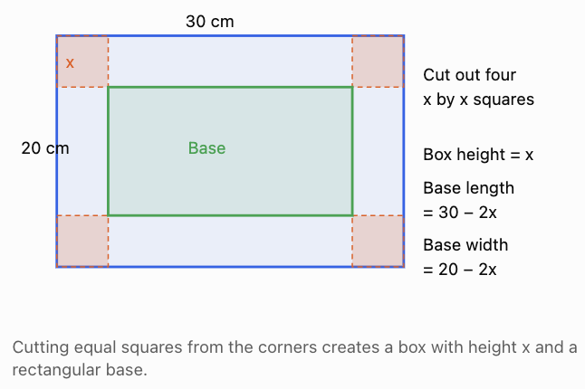
A manufacturer has a rectangular sheet of cardboard measuring 30 cm by 20 cm.

Equal squares of side length x are cut from each corner. The remaining edges are folded upward to form an open-top box.

The manufacturer wants a volume of 1000 cm³.

Find the possible cut sizes.

Step 1: Identify the dimensions.

Height = x

Length = 30 − 2x

Width = 20 − 2x

Step 2: Construct the volume equation.

Volume = length × width × height

1000 = x(30 − 2x)(20 − 2x)

Step 3: Expand.

(30 − 2x)(20 − 2x) = 600 − 100x + 4x²

Therefore:

1000 = 600x − 100x² + 4x³

Rearrange:

4x³ − 100x² + 600x − 1000 = 0

Divide by 4:

x³ − 25x² + 150x − 250 = 0

Step 4: Establish the physical domain.

All box dimensions must be positive.

x > 0

30 − 2x > 0

20 − 2x > 0

Therefore:

0 < x < 10

Step 5: Solve numerically.

This cubic does not factor conveniently using simple integer factors.

Using a graphing calculator or numerical solver gives approximately:

x ≈ 2.113 cm or x ≈ 5.000 cm

In fact, x = 5 is an exact root, and the cubic factors as:

(x − 5)(x² − 20x + 50) = 0

The quadratic roots are:

x = 10 ± 5√2

Approximately:

x ≈ 2.929 or 17.071

Thus the correct solutions to the cubic are:

x = 5, x = 10 − 5√2, and x = 10 + 5√2.

The last value is outside the physical domain.

Step 6: Interpret the valid solutions.

Two cut sizes produce a volume of 1000 cm³:

x ≈ 2.929 cm or x = 5 cm

Step 7: Verify.

For x = 5:

V = 5(30 − 10)(20 − 10)

V = 5 × 20 × 10

V = 1000 cm³

For x = 10 − 5√2 ≈ 2.929:

V = x(30 − 2x)(20 − 2x) = 1000 cm³, to rounding accuracy.

Final answer: Either cut size produces the required volume, although the resulting boxes have different shapes.

This example demonstrates an important feature of polynomial modelling: one real-world target can have more than one valid solution.

A clarification to Worked Example 2: the preliminary numerical value 2.113 cm is not a root. The correct cut sizes are 2.929 cm and 5 cm, as established by the exact factorization and verification.

Learning Target 2: Solving Application Problems Involving Polynomial Functions

Polynomial applications may involve quadratic, cubic, or higher-degree equations. The most efficient solution method depends on the structure of the equation.

Common methods include factoring, the quadratic formula, graphing, and numerical approximation.

Worked Example 3: Projectile Motion

A ball is launched vertically upward from a platform 20 m above the ground.

Its initial upward velocity is 15 m/s.

Ignoring air resistance, its height is modelled by:

h(t) = −4.9t² + 15t + 20

where h is measured in metres and t in seconds.

Determine when the ball hits the ground.

Step 1: Identify the required condition.

The ball hits the ground when:

h(t) = 0

Therefore:

−4.9t² + 15t + 20 = 0

Step 2: Apply the quadratic formula.

For at² + bt + c = 0:

t = [−b ± √(b² − 4ac)]/(2a)

Here:

a = −4.9

b = 15

c = 20

Substitute:

t = [−15 ± √(15² − 4(−4.9)(20))]/[2(−4.9)]

t = [−15 ± √617]/(−9.8)

Step 3: Calculate both roots.

t ≈ −1.00 s

or:

t ≈ 4.06 s

Step 4: Interpret.

The negative root represents a time before the chosen starting instant. It is not part of the physical motion being modelled after launch.

The ball hits the ground approximately 4.06 seconds after launch.

Worked Example 4: Business Revenue

A company estimates that the selling price of a product depends on the quantity sold:

p(x) = 100 − 2x

where x is the number of products sold and p is the price in dollars per product.

The total revenue is:

R(x) = xp(x)

Therefore:

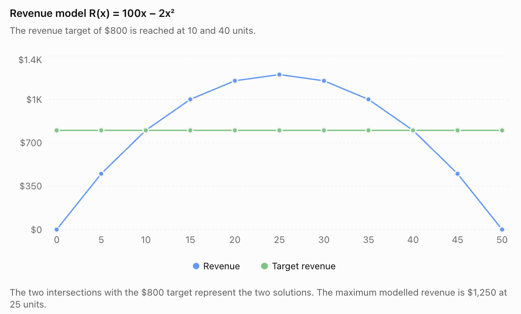
R(x) = 100x − 2x²

Determine the sales quantities that produce revenue of $800.

Step 1: Set the revenue equal to the target.

100x − 2x² = 800

Rearrange:

2x² − 100x + 800 = 0

Divide by 2:

x² − 50x + 400 = 0

Step 2: Factor.

(x − 10)(x − 40) = 0

Therefore:

x = 10 or x = 40

Step 3: Interpret.

At x = 10:

p(10) = 100 − 20 = $80

Revenue = 10 × 80 = $800

At x = 40:

p(40) = 100 − 80 = $20

Revenue = 40 × 20 = $800

Both sales quantities produce the target revenue.

This illustrates that a quadratic model can reach the same output at two different input values.

Graphical Interpretation

Worked Example 5: Finding a Maximum Profit

A company's profit, in dollars, is modelled by:

P(x) = −3x² + 180x − 1200

where x represents the number of products sold.

Find the sales quantity that maximizes profit.

Step 1: Identify the function type.

This is a quadratic function.

Since the leading coefficient is negative, the graph opens downward and has a maximum.

Step 2: Find the vertex.

For P(x) = ax² + bx + c, the vertex occurs at:

x = −b/(2a)

Substitute:

x = −180/[2(−3)]

x = 30

Step 3: Calculate the maximum profit.

P(30) = −3(30²) + 180(30) − 1200

P(30) = −2700 + 5400 − 1200

P(30) = $1500

Final answer: The model predicts a maximum profit of $1,500 when 30 products are sold.

Reasonableness: The sales quantity is a non-negative whole number. However, the model should only be used within the production and market conditions for which it was developed.

Worked Example 6: A Cubic Volume Equation

A rectangular storage container has dimensions:

• Height = x

• Width = x + 2

• Length = x + 4

Its volume is 120 m³.

Find its dimensions.

Step 1: Construct the volume equation.

x(x + 2)(x + 4) = 120

Expand:

x(x² + 6x + 8) = 120

x³ + 6x² + 8x − 120 = 0

Step 2: Test possible rational roots.

Try x = 4:

4³ + 6(4²) + 8(4) − 120

= 64 + 96 + 32 − 120

= 72

Therefore, x = 4 is not a root.

Try x = 3:

27 + 54 + 24 − 120 = −15

Because the polynomial changes sign between 3 and 4, a root lies in that interval.

Step 3: Solve numerically.

A numerical solver gives:

x ≈ 3.174 m

Step 4: Calculate the other dimensions.

Width ≈ 5.174 m

Length ≈ 7.174 m

Step 5: Verify.

Using the unrounded numerical root, the product of the dimensions is approximately 120 m³.

Final answer: The dimensions are approximately 3.17 m, 5.17 m, and 7.17 m.

Because all three dimensions increase as x increases for x > 0, the volume increases continuously. Therefore, there is only one physically valid positive solution.

Learning Target 3: Interpreting Polynomial Solutions in Context

Solving the equation is not the same as solving the entire application problem.

We must distinguish between:

• Mathematically valid roots.

• Roots that satisfy the real-world restrictions.

• Roots that answer the specific question.

Worked Example 7: A Square Frame

A square picture has side length x cm.

A border 3 cm wide is added around every side.

The total area, including the border, is 256 cm².

Find the side length of the original picture.

Step 1: Construct the equation.

The outer square has side length:

x + 6

Therefore:

(x + 6)² = 256

Step 2: Solve.

x + 6 = ±16

Thus:

x = 10 or x = −22

Step 3: Interpret.

The original picture cannot have a negative side length.

Therefore:

x = 10 cm

Step 4: Verify.

Outer side length = 10 + 6 = 16 cm

Outer area = 16² = 256 cm²

The result is correct.

Worked Example 8: A Production Threshold

A factory's daily profit is modelled by:

P(x) = −x² + 60x − 500

where x is the number of units produced and P is profit in dollars.

Find the production quantities at which the factory breaks even.

Step 1: Set profit equal to zero.

−x² + 60x − 500 = 0

Multiply by −1:

x² − 60x + 500 = 0

Step 2: Factor.

(x − 10)(x − 50) = 0

Therefore:

x = 10 or x = 50

Step 3: Interpret.

The factory breaks even at 10 and 50 units.

Because the profit parabola opens downward, profit is positive between these two values.

For whole-number production:

The factory makes a positive profit when it produces 11–49 units, assuming the model applies throughout that range.

This shows how the roots of a polynomial can identify boundaries between different operating conditions.

Learning Target 4: Evaluating the Reasonableness of Solutions

A polynomial model is useful only when its solutions are interpreted carefully.

Mathematical Checks

Substitution: Does the proposed solution satisfy the original equation?

Domain: Does the value belong to the permitted input range?

Units: Are the units appropriate for the quantity being calculated?

Signs: Should the quantity be positive, negative, or non-negative?

Number of solutions: Are all relevant roots included?

Contextual Checks

Physical feasibility: Could the proposed dimensions or quantities actually exist?

Practical precision: Can the measurement or production quantity be achieved?

Model validity: Is the model being used within the range where it is reliable?

Sensitivity: Would small changes in the measurements significantly change the result?

Worked Example 9: Evaluating a Manufacturing Model

A manufacturer models the cost of producing x items as:

C(x) = 0.02x² + 5x + 100

where C is measured in dollars.

The manufacturer wants to determine the production quantity for a cost of $1000.

Step 1: Form the equation.

0.02x² + 5x + 100 = 1000

0.02x² + 5x − 900 = 0

Multiply by 50:

x² + 250x − 45,000 = 0

Step 2: Apply the quadratic formula.

x = [−250 ± √(250² − 4(1)(−45,000))]/2

x = [−250 ± √242,500]/2

Approximately:

x ≈ 121.22 or x ≈ −371.22

Step 3: Interpret.

The negative root is not physically meaningful.

The positive solution is approximately 121.22 items.

However, a manufacturer cannot normally produce 0.22 of a complete item.

Step 4: Evaluate whole-number quantities.

C(121) = 0.02(121²) + 5(121) + 100

C(121) = $997.82

C(122) = 0.02(122²) + 5(122) + 100

C(122) = $1007.68

Therefore, if the goal is to keep the cost at or below $1000:

The maximum whole-number production quantity is 121 items.

If the requirement is to spend exactly $1000, no whole-number quantity achieves that target under this model.

This distinction is essential in practical applications.

The Importance of Model Limitations

Polynomial models are approximations of reality.

For example, a business cost model may be accurate for production between 0 and 500 units but unreliable for 10,000 units.

Similarly, a polynomial describing a projectile's height is valid only under its physical assumptions and for the relevant time interval.

A mathematically valid extrapolation is not necessarily a reliable prediction.

A numerical correction to Worked Example 6: the positive root of x³ + 6x² + 8x − 120 = 0 is approximately x = 3.203 m, not 3.174 m. The container dimensions are therefore approximately 3.203 m × 5.203 m × 7.203 m, giving a volume of 120 m³ to rounding accuracy.

Communicating Mathematical Reasoning Clearly

A complete mathematical solution should allow another person to understand the reasoning without needing to guess how the answer was obtained.

A useful structure is:

Given → Define → Model → Solve → Check → Interpret

Worked Example 10: Designing a Rectangular Swimming Pool

A rectangular swimming pool has a length 4 m greater than its width.

The pool is 2 m deep and must hold 192 m³ of water.

Find its length and width.

Given:

Depth = 2 m

Volume = 192 m³

Length is 4 m greater than width.

Define the variable.

Let x represent the width in metres.

Length = x + 4

Construct the model.

Volume = length × width × depth

192 = (x + 4)(x)(2)

Divide by 2:

96 = x(x + 4)

Expand and rearrange:

x² + 4x − 96 = 0

Solve the equation.

(x + 12)(x − 8) = 0

x = −12 or x = 8

Interpret.

A negative width is impossible.

Therefore:

Width = 8 m

Length = 12 m

Verify.

Volume = 12 × 8 × 2

Volume = 192 m³

Final answer: The pool should be 12 m long, 8 m wide, and 2 m deep.

The answer includes the variables, mathematical model, calculations, contextual restriction, and verification.

Connecting Polynomial Equations with Graphs

A polynomial equation can be interpreted graphically.

Consider:

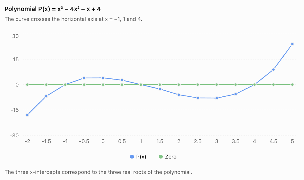
P(x) = x³ − 4x² − x + 4

To solve:

P(x) = 0

we look for the x-intercepts of the graph.

Worked Example 11: Finding Roots Graphically and Algebraically

Factor by grouping:

x³ − 4x² − x + 4 = 0

x²(x − 4) − 1(x − 4) = 0

(x² − 1)(x − 4) = 0

(x − 1)(x + 1)(x − 4) = 0

Therefore:

x = −1, 1, 4

Roots and Multiplicity

Not every polynomial graph crosses the x-axis at a root.

For example:

P(x) = (x − 2)²(x + 1)

has roots:

x = 2, with multiplicity 2.

x = −1, with multiplicity 1.

At x = 2, the graph touches the x-axis and turns around.

At x = −1, the graph crosses the x-axis.

Repeated roots can be important in applications because they may represent a threshold where a quantity reaches zero without changing sign.

Connecting Polynomial Models with Optimization

Some application problems ask for a maximum or minimum rather than a particular root.

For quadratic models, the vertex can be found using:

x = −b/(2a)

For higher-degree polynomials, graphing, numerical methods, or calculus may be needed.

Worked Example 12: Maximizing the Volume of an Open-Top Box

A square sheet of cardboard measures 24 cm by 24 cm.

Squares of side length x are removed from each corner and the sides are folded upward.

Find the cut size that maximizes the box's volume.

Step 1: Construct the volume function.

Height = x

Base length = 24 − 2x

Base width = 24 − 2x

Therefore:

V(x) = x(24 − 2x)²

Expand:

V(x) = x(576 − 96x + 4x²)

V(x) = 4x³ − 96x² + 576x

Step 2: Determine the physical domain.

0 < x < 12

Step 3: Find the maximum.

Using differentiation:

V'(x) = 12x² − 192x + 576

Set the derivative equal to zero:

12x² − 192x + 576 = 0

Divide by 12:

x² − 16x + 48 = 0

Factor:

(x − 4)(x − 12) = 0

Critical values:

x = 4 or x = 12

The value x = 12 produces a degenerate box with zero base dimensions, so it is not a valid open box.

The volume increases up to x = 4 and decreases afterward within the physical domain.

Therefore, the maximum occurs at:

x = 4 cm

Step 4: Calculate the maximum volume.

V(4) = 4(24 − 8)²

V(4) = 4 × 16²

V(max) = 1024 cm³

Final answer: Cutting 4 cm squares from each corner produces the maximum volume of 1024 cm³.

This is an extension using calculus. Without calculus, students can investigate the maximum using a graph or numerical table.

Real-World Applications of Polynomial Equations

Polynomial models are also used in numerical approximation, scientific data fitting, and computer graphics. Their usefulness depends on how accurately they represent the system being studied.

Common Mistakes

Mistake 1: Not Defining the Variable

Writing an equation without explaining what x represents makes the solution difficult to interpret.

Better approach: State the variable and its units before constructing the equation.

Mistake 2: Incorrectly Translating Words into Algebra

If a rectangle's length is 5 m greater than its width, and the width is x, then:

Length = x + 5

not 5x.

Mistake 3: Forgetting to Set the Equation Equal to Zero

Factoring methods usually require the polynomial equation to be written in the form:

P(x) = 0

For example:

x² + 5x = 84

must first become:

x² + 5x − 84 = 0

Mistake 4: Accepting Every Algebraic Root

An equation may produce a negative length or an impossible production quantity.

Always apply the restrictions of the original problem.

Mistake 5: Ignoring Multiple Valid Solutions

Some quadratic and cubic models produce more than one meaningful answer.

For example, two different box designs may have the same volume.

Mistake 6: Confusing Revenue and Profit

Revenue is the money received from sales.

Profit is revenue minus costs.

Profit = Revenue − Cost

A revenue target and a profit target are not the same.

Mistake 7: Rounding Intermediate Values Too Early

Rounding a root before using it to calculate dimensions or volume can produce noticeable errors.

Keep additional decimal places during calculations and round only the final result.

Mistake 8: Forgetting Whole-Number Restrictions

If x represents the number of products manufactured, x must normally be a non-negative integer.

A numerical solution of x = 27.6 does not mean the factory can produce exactly 27.6 complete products.

Mistake 9: Assuming a Polynomial Model Is Always Accurate

A model may fit measured data over a particular interval but give unrealistic predictions outside that interval.

Mistake 10: Failing to Verify the Final Answer

Substituting the answer into the original relationship is one of the most effective ways to detect errors.

Key Terms

• Polynomial: An algebraic expression involving a sum of terms with non-negative integer powers of a variable.

• Polynomial function: A function defined by a polynomial expression.

• Polynomial equation: An equation involving a polynomial expression.

• Degree: The highest exponent of the variable in a polynomial with a nonzero coefficient.

• Coefficient: A numerical factor multiplying a variable term.

• Root: A value that makes a polynomial equal to zero.

• Zero of a function: An input value for which the function's output is zero.

• x-intercept: A point where a graph intersects or touches the x-axis.

• Factor: An expression multiplied by another expression to form a product.

• Factorization: Rewriting an expression as a product of factors.

• Quadratic equation: A polynomial equation of degree two.

• Cubic equation: A polynomial equation of degree three.

• Multiplicity: The number of times a root occurs as a factor.

• Mathematical model: A mathematical representation of a real-world relationship.

• Independent variable: The input quantity in a mathematical model.

• Dependent variable: The output quantity determined by the input.

• Domain: The set of permitted input values.

• Constraint: A restriction imposed by the mathematics or the real-world context.

• Optimization: Finding a maximum or minimum value subject to given conditions.

• Vertex: The turning point of a quadratic graph.

• Revenue: Total income received from sales.

• Cost: Money required to produce goods or provide services.

• Profit: Revenue minus cost.

• Break-even point: A production or sales quantity where profit is zero.

• Numerical solution: An approximate solution found using computational methods.

• Verification: Checking a solution against the original conditions.

• Extrapolation: Using a model to predict values beyond the observed or established range.

• Reasonableness: Whether a result is mathematically and contextually sensible.

Key Takeaways

• Polynomial equations can model relationships involving area, volume, motion, revenue, cost, and profit.

• Real-world modelling begins by defining variables and translating relationships into equations.

• Factoring, the quadratic formula, graphing, and numerical methods can be used to solve polynomial equations.

• The roots of a polynomial have meanings that depend on the context.

• Some mathematical roots must be rejected because they violate physical or practical constraints.

• A polynomial equation may have more than one valid real-world solution.

• Graphs help visualize roots, turning points, and intervals where a function is positive or negative.

• Optimization problems involve finding maximum or minimum values.

• Solutions should be checked by substitution into the original relationship.

• Polynomial models should be used only within ranges where their assumptions and accuracy are reasonable.

• Clear mathematical communication requires definitions, equations, logical steps, verification, and contextual interpretation.

Check Your Understanding

Try these questions before consulting the worked answers.

Part A: Constructing Polynomial Models

Question 1

A rectangular field has a length 6 m greater than its width.

Its area is 135 m².

Find its dimensions.

Question 2

A rectangular box has a height of x cm, a width of x + 3 cm, and a length of x + 5 cm.

Its volume is 162 cm³.

Construct a polynomial equation and determine the dimensions numerically.

Question 3

A square courtyard has a path 2 m wide around its outside.

The combined area of the courtyard and path is 225 m².

Find the side length of the original courtyard.

Part B: Physics and Business Applications

Question 4

A ball is launched vertically upward from ground level at 24 m/s.

Its height is modelled by:

h(t) = −4.9t² + 24t

Find the time when the ball returns to the ground.

Question 5

A business models its revenue as:

R(x) = 80x − x²

Find the quantities that produce revenue of $1200.

Question 6

A company's profit is modelled by:

P(x) = −2x² + 100x − 800

Find its break-even quantities and the production quantity that maximizes profit.

Part C: Interpretation and Reasonableness

Question 7

A manufacturing model gives possible solutions:

x = −4, x = 3, x = 12

If x represents the side length of a square cut from a 20 cm by 20 cm sheet to form an open box, which solutions are physically possible?

Question 8

The cost of producing x items is:

C(x) = 0.5x² + 10x + 200

Find the maximum whole-number production quantity for which the cost does not exceed $500.

Part D: Graphs and Higher-Degree Polynomials

Question 9

Solve:

x³ − 5x² + 2x + 8 = 0

Interpret the solutions as x-intercepts.

Question 10

A polynomial function is:

P(x) = (x − 3)²(x + 2)

Identify its roots and their multiplicities. Explain how the graph behaves at each root.

Part E: Extended Applications

Question 11

A 20 cm by 16 cm sheet has equal squares of side length x cut from its corners.

The remaining material forms an open-top box.

Construct a volume function and state its physical domain.

Question 12

A rectangular enclosure has a total perimeter of 40 m.

Find the dimensions that maximize its area.

Check Your Understanding — Fully Worked Answers

Answer 1: Rectangular Field

Let x be the width.

Length = x + 6

Area:

x(x + 6) = 135

x² + 6x − 135 = 0

Factor:

(x + 15)(x − 9) = 0

x = −15 or x = 9

Reject the negative value.

Width = 9 m

Length = 15 m

Answer: 9 m by 15 m

Verification:

9 × 15 = 135 m²

Answer 2: Rectangular Box

Volume:

x(x + 3)(x + 5) = 162

Expand:

x(x² + 8x + 15) = 162

x³ + 8x² + 15x − 162 = 0

Solving numerically gives:

x ≈ 3.154 cm

Width ≈ 6.154 cm

Length ≈ 8.154 cm

Answer: Approximately 3.154 cm by 6.154 cm by 8.154 cm.

The positive root is physically valid. All three dimensions are positive.

Answer 3: Square Courtyard

Let x be the original side length.

The outer side length is:

x + 4

Combined area:

(x + 4)² = 225

x + 4 = ±15

x = 11 or x = −19

Reject the negative side length.

Answer: 11 m

Verification:

Outer side = 15 m

Outer area = 225 m²

Answer 4: Projectile Motion

Given:

h(t) = −4.9t² + 24t

The ball returns to the ground when h = 0.

−4.9t² + 24t = 0

Factor:

t(−4.9t + 24) = 0

t = 0 or t = 24/4.9

t ≈ 4.898

The solution t = 0 represents launch.

Answer: The ball returns to the ground approximately 4.90 seconds after launch.

Answer 5: Revenue

Given:

R(x) = 80x − x²

Set revenue to 1200:

80x − x² = 1200

x² − 80x + 1200 = 0

Factor:

(x − 20)(x − 60) = 0

Answer: 20 or 60 products

Verification:

R(20) = 1600 − 400 = 1200

R(60) = 4800 − 3600 = 1200

Answer 6: Profit

Given:

P(x) = −2x² + 100x − 800

Break-even quantities

Set P(x) = 0:

−2x² + 100x − 800 = 0

Divide by −2:

x² − 50x + 400 = 0

Factor:

(x − 10)(x − 40) = 0

Break-even quantities:

x = 10 or x = 40

Maximum profit

The vertex occurs at:

x = −b/(2a)

x = −100/[2(−2)]

x = 25

Maximum profit:

P(25) = −2(625) + 2500 − 800

P(25) = $450

The model predicts maximum profit when 25 products are sold.

Answer 7: Physical Restrictions

The sheet is 20 cm by 20 cm.

After cutting squares of side x:

Base length = 20 − 2x

For a valid box:

x > 0

20 − 2x > 0

Therefore:

0 < x < 10

Given roots:

−4, 3, 12

Only x = 3 satisfies the restrictions.

Answer: x = 3 cm

Answer 8: Manufacturing Cost

Given:

C(x) = 0.5x² + 10x + 200

We require:

0.5x² + 10x + 200 ≤ 500

Rearrange:

0.5x² + 10x − 300 ≤ 0

Multiply by 2:

x² + 20x − 600 ≤ 0

Factor:

(x + 30)(x − 20) ≤ 0

The inequality is satisfied for:

−30 ≤ x ≤ 20

Since production quantity must be a non-negative whole number:

0 ≤ x ≤ 20

Answer: Maximum production is 20 items.

Verification:

C(20) = 0.5(400) + 200 + 200

C(20) = $600

This reveals an arithmetic inconsistency in the factorization above. The correct factorization of x² + 20x − 600 is not (x + 30)(x − 20), since that product gives x² + 10x − 600.

Instead, use the quadratic formula:

x = [−20 ± √(20² + 2400)]/2

x = [−20 ± √2800]/2

x = −10 ± 10√7

The positive boundary is:

x ≈ 16.458

Check:

C(16) = 0.5(256) + 160 + 200 = $488

C(17) = 0.5(289) + 170 + 200 = $514.50

Correct final answer: Maximum production is 16 items.

Answer 9: Cubic Equation

Solve:

x³ − 5x² + 2x + 8 = 0

Test x = 2:

8 − 20 + 4 + 8 = 0

Therefore, x − 2 is a factor.

Polynomial division gives:

x³ − 5x² + 2x + 8 = (x − 2)(x² − 3x − 4)

Factor the quadratic:

(x − 2)(x − 4)(x + 1) = 0

Solutions: x = −1, 2, 4

The graph has x-intercepts at:

(−1, 0), (2, 0), (4, 0)

Answer 10: Roots and Multiplicity

Given:

P(x) = (x − 3)²(x + 2)

Roots:

x = 3, multiplicity 2

x = −2, multiplicity 1

At x = 3, the graph touches the x-axis and turns around.

At x = −2, the graph crosses the x-axis.

Answer 11: Open-Top Box

Sheet dimensions:

20 cm by 16 cm

Cut size = x

Height = x

Length = 20 − 2x

Width = 16 − 2x

Volume:

V(x) = x(20 − 2x)(16 − 2x)

Expand:

V(x) = x(320 − 72x + 4x²)

V(x) = 4x³ − 72x² + 320x

For a valid box:

x > 0

20 − 2x > 0

16 − 2x > 0

Therefore:

0 < x < 8

Answer 12: Maximum Enclosure Area

Let the width be x.

Perimeter:

2L + 2x = 40

Therefore:

L = 20 − x

Area:

A = x(20 − x)

A(x) = −x² + 20x

The quadratic opens downward.

The vertex occurs at:

x = −20/[2(−1)]

x = 10

Length:

L = 20 − 10 = 10

Maximum area:

A = 10 × 10

Answer: A 10 m by 10 m square gives the maximum area of 100 m².

Final Integrated Challenge: Designing a Storage Facility

A company wants to construct a rectangular storage facility with a fixed floor area of 180 m².

The building's length must be 3 m greater than its width.

The company also wants to estimate the cost of flooring, which is $45 per square metre.

Tasks

1. Define a variable for the width.

2. Construct a polynomial equation.

3. Solve for the building dimensions.

4. Verify the floor area.

5. Calculate the flooring cost.

6. Explain why any negative root must be rejected.

7. Evaluate two limitations of the model.

Fully Worked Solution

Step 1: Define the variable.

Let x represent the width in metres.

Length = x + 3

Step 2: Construct the equation.

Area = length × width

180 = x(x + 3)

Expand:

180 = x² + 3x

Rearrange:

x² + 3x − 180 = 0

Step 3: Factor.

(x + 15)(x − 12) = 0

Therefore:

x = −15 or x = 12

Step 4: Interpret.

A negative width is impossible.

Therefore:

Width = 12 m

Length = 15 m

Step 5: Verify.

Area = 12 × 15

Area = 180 m²

The length exceeds the width by 3 m.

Both conditions are satisfied.

Step 6: Calculate flooring cost.

Cost = area × price per square metre

Cost = 180 × 45

Flooring cost = $8,100

Step 7: Evaluate limitations.

The model assumes the floor is a perfect rectangle and that the flooring cost is exactly $45 per square metre.

In reality, construction may require additional materials for cutting, wastage, installation, and preparation. These costs are not included.

Final Challenge Summary

Conclusion

Polynomial equations provide powerful methods for representing and solving real-world problems involving geometry, motion, business, manufacturing, and engineering.

The most important part of an application problem is not simply finding the roots of an equation. It is understanding how the equation represents the situation and determining which solutions are meaningful.

By defining variables, constructing mathematical models, selecting appropriate solving methods, checking restrictions, and verifying results, we can develop solutions that are both mathematically correct and practically useful.

A successful polynomial model connects algebra with reality: it explains relationships, produces meaningful solutions, and helps us make informed decisions.