Polynomial Graph Analysis

Introduction

Polynomial graphs provide a visual way to understand how mathematical functions behave. By examining a graph, we can identify where a function equals zero, where it reaches high or low values, where it increases or decreases, and how its values change over different intervals.

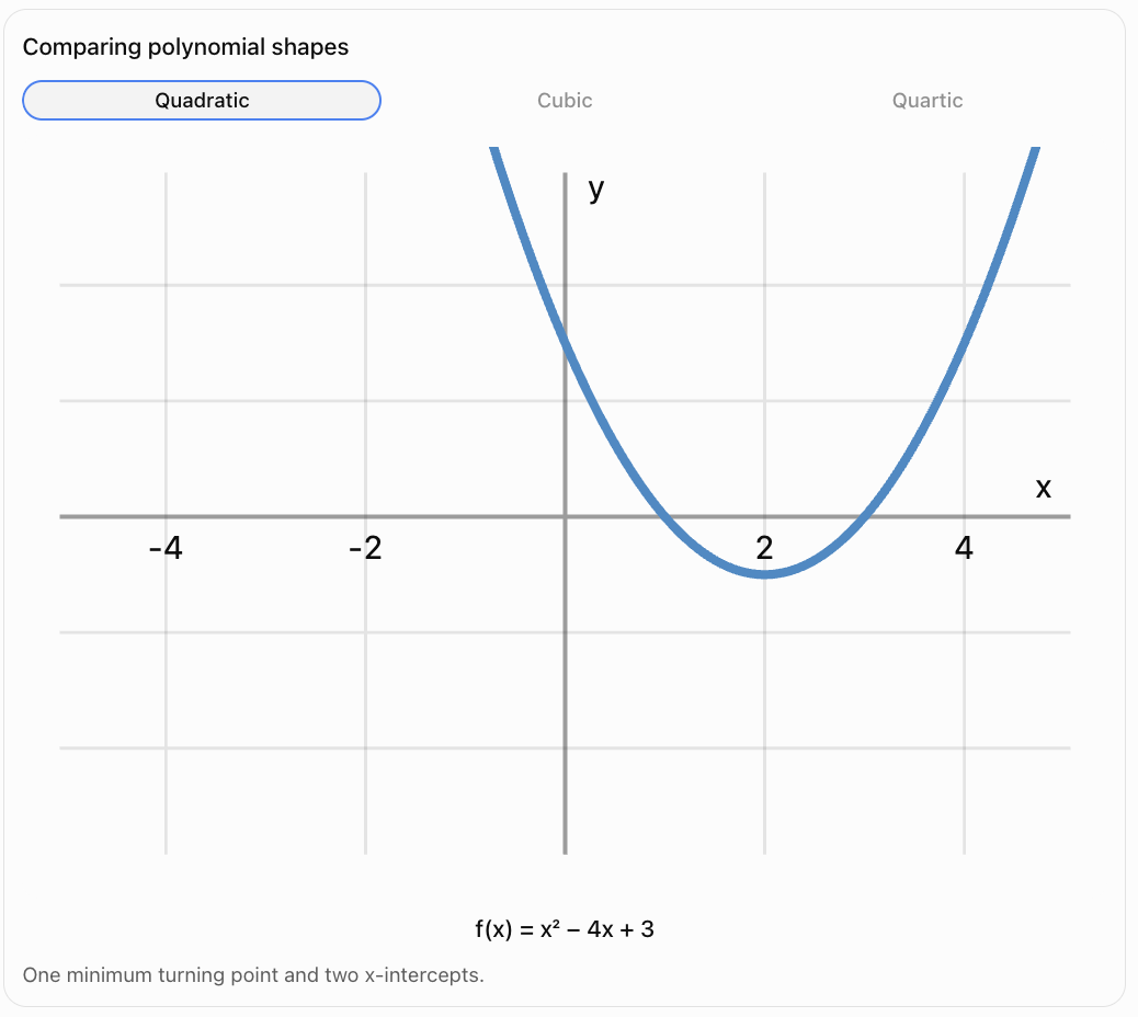
For example, consider the quadratic function:

f(x) = x² − 4x + 3

Factoring gives:

f(x) = (x − 1)(x − 3)

From the equation, we can determine that the graph:

• Crosses the x-axis at x = 1 and x = 3.

• Crosses the y-axis at y = 3.

• Opens upward because the leading coefficient is positive.

• Has a minimum turning point at (2, −1).

• Decreases before x = 2 and increases after x = 2.

These features allow us to sketch the graph accurately without plotting a large number of points.

Polynomial graph analysis is important in algebra, calculus, physics, economics, engineering, and mathematical modelling.

What Is a Polynomial Function?

A polynomial function is a function that can be written in the form:

f(x) = aₙxⁿ + aₙ₋₁xⁿ⁻¹ + ... + a₂x² + a₁x + a₀

where:

• n is a nonnegative integer.

• The coefficients are real numbers for the graphs considered here.

• aₙ ≠ 0.

• The highest exponent n is the degree of the polynomial.

Examples include:

• Linear: f(x) = 2x + 1

• Quadratic: f(x) = x² − 4x + 3

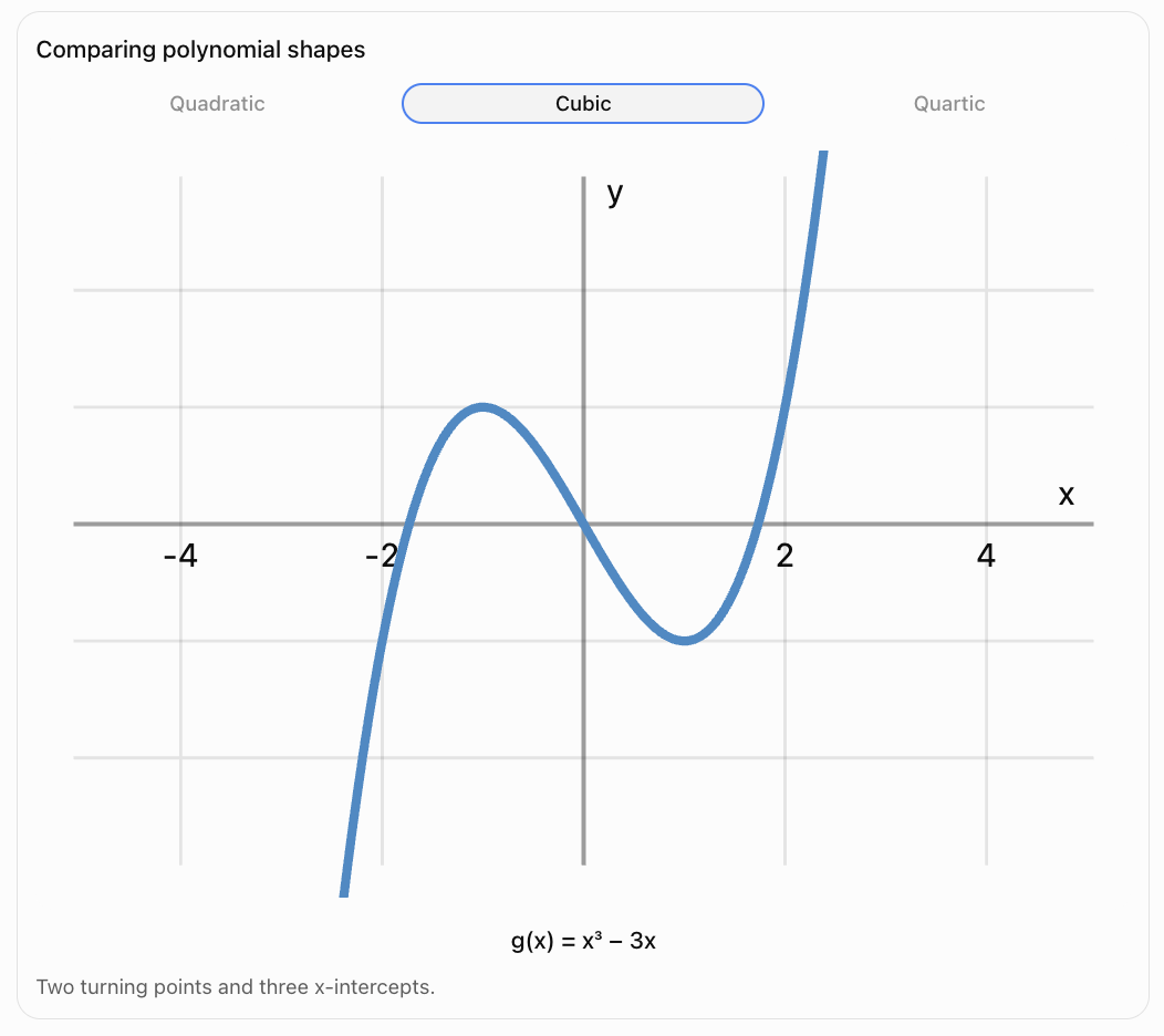
• Cubic: f(x) = x³ − 3x

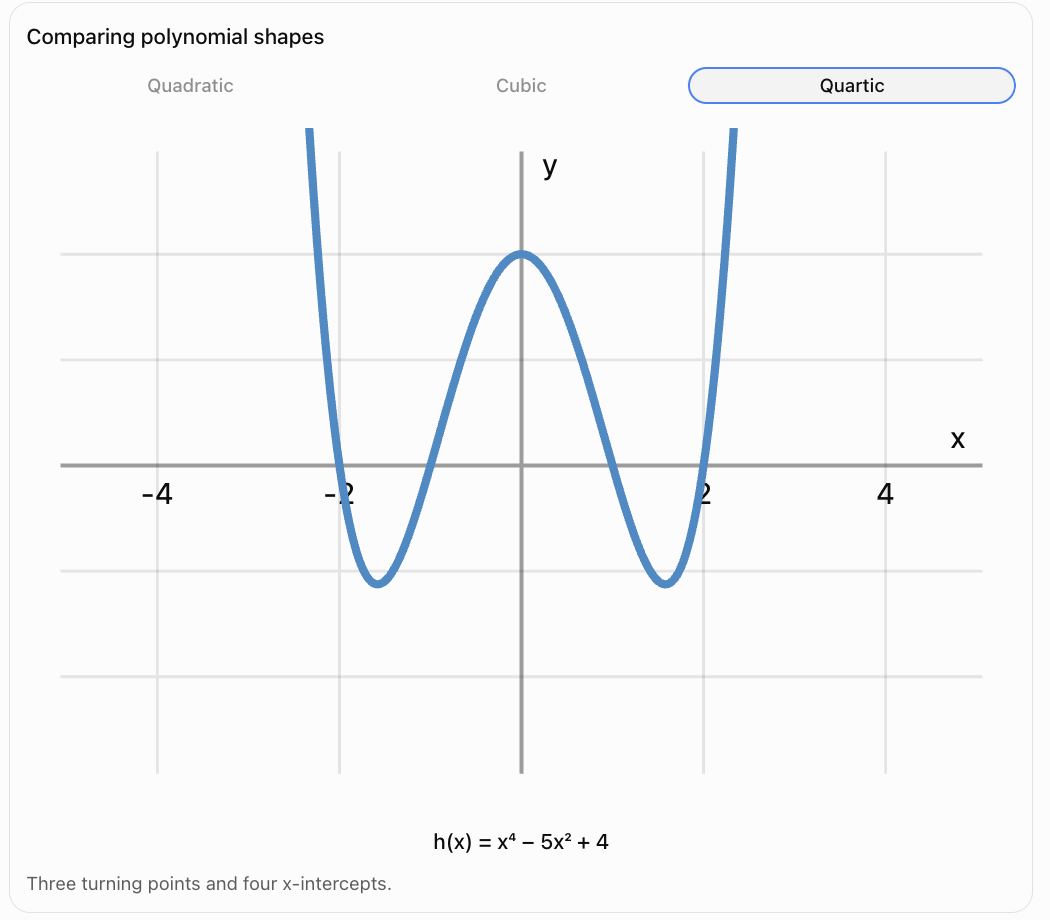
• Quartic: f(x) = x⁴ − 5x² + 4

• Quintic: f(x) = x⁵ − 4x³

Polynomial graphs are continuous and smooth. They have no breaks, holes, jumps, or sharp corners.

Every polynomial function has a domain of all real numbers.

Understanding the Key Features of a Polynomial Graph

When analysing a polynomial graph, we usually examine several important features.

These features work together to help us sketch and interpret polynomial functions.

Finding the y-Intercept

The y-intercept is the point where the graph crosses the y-axis.

At every point on the y-axis:

x = 0

Therefore, to find the y-intercept, substitute x = 0 into the function.

Worked Example

Find the y-intercept of:

f(x) = 2x³ − 5x² + 4x − 7

Substitute x = 0:

f(0) = 2(0)³ − 5(0)² + 4(0) − 7

f(0) = −7

Therefore:

The y-intercept is (0, −7).

Another Example

Find the y-intercept of:

f(x) = −3x⁴ + 2x² + 8

Substitute x = 0:

f(0) = 8

Therefore:

The y-intercept is (0, 8).

Shortcut

For a polynomial written in standard form, the y-intercept is the constant term.

For example:

f(x) = 5x⁴ − 3x² + 2x + 9

The y-intercept is:

(0, 9)

This shortcut works because all terms containing x become zero when x = 0.

Finding the x-Intercepts

The x-intercepts are the points where the graph meets the x-axis.

At every point on the x-axis:

y = 0

Therefore, to find the x-intercepts, solve:

f(x) = 0

Worked Example

Find the x-intercepts of:

f(x) = x² − 5x + 6

Set the function equal to zero:

x² − 5x + 6 = 0

Factor:

(x − 2)(x − 3) = 0

Apply the zero product property:

x − 2 = 0

or:

x − 3 = 0

Therefore:

x = 2 or x = 3

The x-intercepts are:

(2, 0) and (3, 0)

Another Example

Find the x-intercepts of:

f(x) = x³ − 4x

Set equal to zero:

x³ − 4x = 0

Factor out x:

x(x² − 4) = 0

Factor the difference of squares:

x(x − 2)(x + 2) = 0

Therefore:

x = 0, 2, or −2

The x-intercepts are:

(−2, 0), (0, 0), and (2, 0)

Important Observation

A polynomial of degree n can have at most n distinct real x-intercepts.

Some polynomials have fewer.

For example:

f(x) = x² + 4

has no real roots and therefore no x-intercepts.

Roots, Zeros, and x-Intercepts

These terms describe related concepts.

Consider:

f(x) = (x − 1)(x + 3)

The roots or zeros are:

x = 1 and x = −3

The x-intercepts are:

(1, 0) and (−3, 0)

The distinction is:

• A root or zero is an x-value.

• An x-intercept is a point on the graph.

Why This Matters

When asked for roots, write:

x = 1, −3

When asked for x-intercepts, write:

(1, 0), (−3, 0)

Both describe where the polynomial equals zero, but the notation is different.

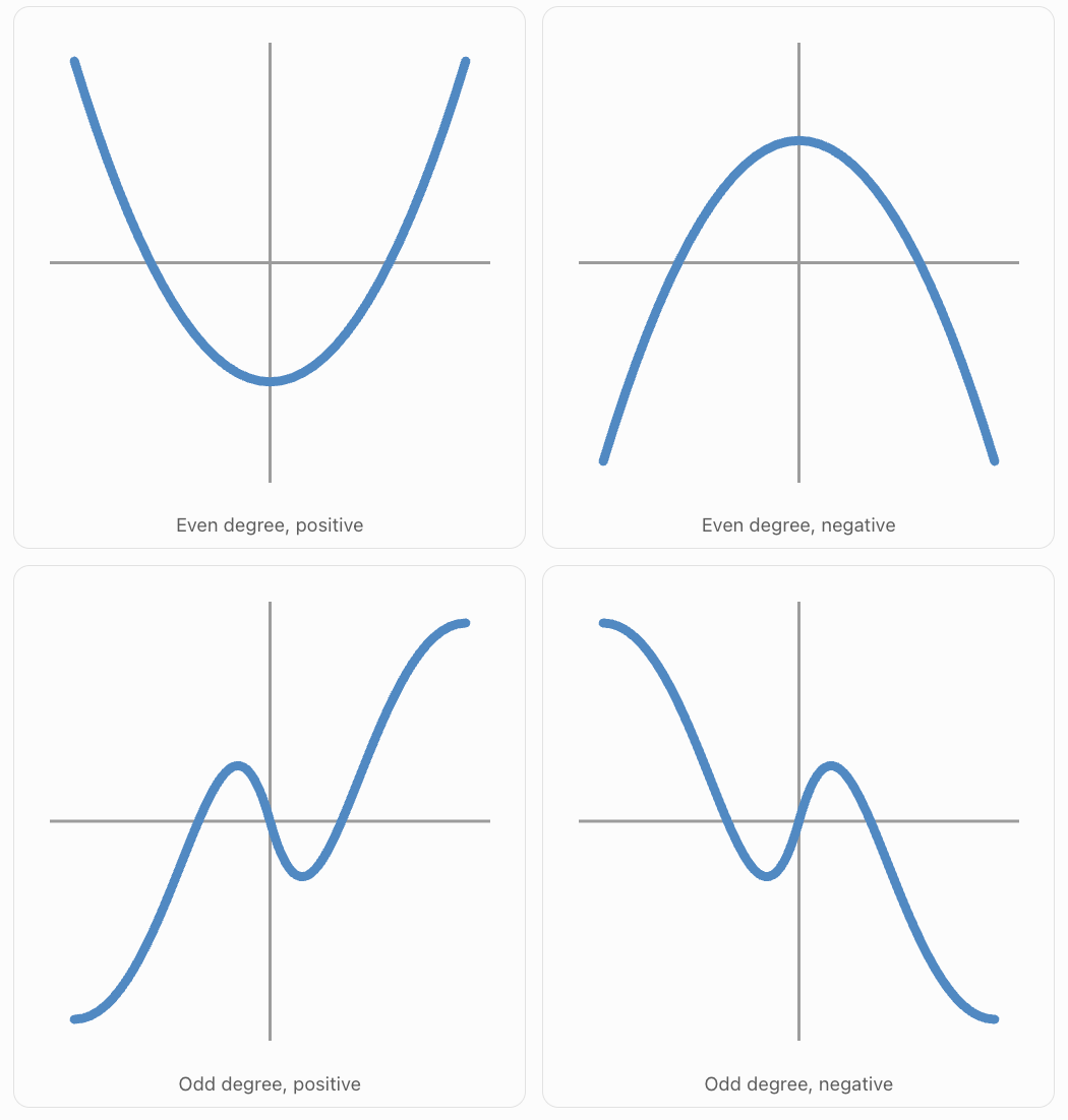
Understanding End Behaviour

The end behaviour of a polynomial describes what happens to the graph as x approaches positive or negative infinity.

The degree and leading coefficient determine the end behaviour.

Even Degree with a Positive Leading Coefficient

Examples:

f(x) = x²

f(x) = 2x⁴ − 3x² + 1

Both ends rise.

As x → −∞, f(x) → +∞.

As x → +∞, f(x) → +∞.

Even Degree with a Negative Leading Coefficient

Examples:

f(x) = −x²

f(x) = −3x⁴ + 2x

Both ends fall.

As x → −∞, f(x) → −∞.

As x → +∞, f(x) → −∞.

Odd Degree with a Positive Leading Coefficient

Examples:

f(x) = x³

f(x) = 2x⁵ − 3x²

The left end falls and the right end rises.

As x → −∞, f(x) → −∞.

As x → +∞, f(x) → +∞.

Odd Degree with a Negative Leading Coefficient

Examples:

f(x) = −x³

f(x) = −4x⁵ + x

The left end rises and the right end falls.

As x → −∞, f(x) → +∞.

As x → +∞, f(x) → −∞.

Polynomial Graph Analysis

Introduction

Polynomial graphs provide a visual way to understand how mathematical functions behave. By examining a graph, we can identify where a function equals zero, where it reaches high or low values, where it increases or decreases, and how its values change over different intervals.

For example, consider the quadratic function:

f(x) = x² − 4x + 3

Factoring gives:

f(x) = (x − 1)(x − 3)

From the equation, we can determine that the graph:

• Crosses the x-axis at x = 1 and x = 3.

• Crosses the y-axis at y = 3.

• Opens upward because the leading coefficient is positive.

• Has a minimum turning point at (2, −1).

• Decreases before x = 2 and increases after x = 2.

These features allow us to sketch the graph accurately without plotting a large number of points.

Polynomial graph analysis is important in algebra, calculus, physics, economics, engineering, and mathematical modelling.

What Is a Polynomial Function?

A polynomial function is a function that can be written in the form:

f(x) = aₙxⁿ + aₙ₋₁xⁿ⁻¹ + ... + a₂x² + a₁x + a₀

where:

• n is a nonnegative integer.

• The coefficients are real numbers for the graphs considered here.

• aₙ ≠ 0.

• The highest exponent n is the degree of the polynomial.

Examples include:

• Linear: f(x) = 2x + 1

• Quadratic: f(x) = x² − 4x + 3

• Cubic: f(x) = x³ − 3x

• Quartic: f(x) = x⁴ − 5x² + 4

• Quintic: f(x) = x⁵ − 4x³

Polynomial graphs are continuous and smooth. They have no breaks, holes, jumps, or sharp corners.

Every polynomial function has a domain of all real numbers.

Understanding the Key Features of a Polynomial Graph

When analysing a polynomial graph, we usually examine several important features.

These features work together to help us sketch and interpret polynomial functions.

Finding the y-Intercept

The y-intercept is the point where the graph crosses the y-axis.

At every point on the y-axis:

x = 0

Therefore, to find the y-intercept, substitute x = 0 into the function.

Worked Example

Find the y-intercept of:

f(x) = 2x³ − 5x² + 4x − 7

Substitute x = 0:

f(0) = 2(0)³ − 5(0)² + 4(0) − 7

f(0) = −7

Therefore:

The y-intercept is (0, −7).

Another Example

Find the y-intercept of:

f(x) = −3x⁴ + 2x² + 8

Substitute x = 0:

f(0) = 8

Therefore:

The y-intercept is (0, 8).

Shortcut

For a polynomial written in standard form, the y-intercept is the constant term.

For example:

f(x) = 5x⁴ − 3x² + 2x + 9

The y-intercept is:

(0, 9)

This shortcut works because all terms containing x become zero when x = 0.

Finding the x-Intercepts

The x-intercepts are the points where the graph meets the x-axis.

At every point on the x-axis:

y = 0

Therefore, to find the x-intercepts, solve:

f(x) = 0

Worked Example

Find the x-intercepts of:

f(x) = x² − 5x + 6

Set the function equal to zero:

x² − 5x + 6 = 0

Factor:

(x − 2)(x − 3) = 0

Apply the zero product property:

x − 2 = 0

or:

x − 3 = 0

Therefore:

x = 2 or x = 3

The x-intercepts are:

(2, 0) and (3, 0)

Another Example

Find the x-intercepts of:

f(x) = x³ − 4x

Set equal to zero:

x³ − 4x = 0

Factor out x:

x(x² − 4) = 0

Factor the difference of squares:

x(x − 2)(x + 2) = 0

Therefore:

x = 0, 2, or −2

The x-intercepts are:

(−2, 0), (0, 0), and (2, 0)

Important Observation

A polynomial of degree n can have at most n distinct real x-intercepts.

Some polynomials have fewer.

For example:

f(x) = x² + 4

has no real roots and therefore no x-intercepts.

Roots, Zeros, and x-Intercepts

These terms describe related concepts.

Consider:

f(x) = (x − 1)(x + 3)

The roots or zeros are:

x = 1 and x = −3

The x-intercepts are:

(1, 0) and (−3, 0)

The distinction is:

• A root or zero is an x-value.

• An x-intercept is a point on the graph.

Why This Matters

When asked for roots, write:

x = 1, −3

When asked for x-intercepts, write:

(1, 0), (−3, 0)

Both describe where the polynomial equals zero, but the notation is different.

Understanding End Behaviour

The end behaviour of a polynomial describes what happens to the graph as x approaches positive or negative infinity.

The degree and leading coefficient determine the end behaviour.

Even Degree with a Positive Leading Coefficient

Examples:

f(x) = x²

f(x) = 2x⁴ − 3x² + 1

Both ends rise.

As x → −∞, f(x) → +∞.

As x → +∞, f(x) → +∞.

Even Degree with a Negative Leading Coefficient

Examples:

f(x) = −x²

f(x) = −3x⁴ + 2x

Both ends fall.

As x → −∞, f(x) → −∞.

As x → +∞, f(x) → −∞.

Odd Degree with a Positive Leading Coefficient

Examples:

f(x) = x³

f(x) = 2x⁵ − 3x²

The left end falls and the right end rises.

As x → −∞, f(x) → −∞.

As x → +∞, f(x) → +∞.

Odd Degree with a Negative Leading Coefficient

Examples:

f(x) = −x³

f(x) = −4x⁵ + x

The left end rises and the right end falls.

As x → −∞, f(x) → +∞.

As x → +∞, f(x) → −∞.

Questions to Consider

How does the maximum possible number of turning points change as the degree increases?

Why do the quadratic and quartic examples have both ends pointing in the same direction?

Why does the cubic example have opposite end behaviour?

How does the number of x-intercepts compare with the degree?

Using Tables of Values to Estimate Graph Features

Sometimes the polynomial cannot be factored easily, or its turning points are difficult to calculate exactly.

A table of values can help.

Worked Example

Consider:

f(x) = x³ − 2x² − x + 2

Construct a table.

The table reveals several useful features:

• The function has zeros at x = −1, 1, and 2.

• The y-intercept is (0, 2).

• The graph rises from x = −1 to x = 0.

• The graph eventually rises again after x = 2.

However, the table alone does not show the exact locations of turning points.

Improve the Estimate

We can calculate more values between the known points.

For example:

f(−0.5) = 1.875

f(0.5) = 1.125

This suggests that a local maximum occurs between −0.5 and 0.5.

To identify the turning points more accurately, use smaller intervals or graphing technology.

Important Limitation

A table shows selected points, not every point on the graph.

Turning points or roots can occur between the values in the table.

Recognising Symmetry in Polynomial Graphs

Symmetry can make graph analysis much easier.

Even Functions

A function is even if:

f(−x) = f(x)

Its graph is symmetric about the y-axis.

Example:

f(x) = x⁴ − 5x² + 4

All powers of x are even.

Therefore:

f(−x) = f(x)

Odd Functions

A function is odd if:

f(−x) = −f(x)

Its graph has rotational symmetry of 180° about the origin.

Example:

f(x) = x³ − 4x

Substitute −x:

f(−x) = −x³ + 4x

= −(x³ − 4x)

= −f(x)

Therefore, the function is odd.

Important Observation

A polynomial containing only even powers of x, including a constant term, is an even function.

A polynomial containing only odd powers of x is an odd function.

A polynomial containing both even and odd powers is generally neither.

Interpreting Positive and Negative Function Values

Polynomial graphs also show where a function is positive or negative.

Positive Intervals

The function is positive where:

f(x) > 0

The graph lies above the x-axis.

Negative Intervals

The function is negative where:

f(x) < 0

The graph lies below the x-axis.

Worked Example

Consider:

f(x) = (x − 1)(x − 3)

The roots are:

x = 1 and x = 3

These roots divide the number line into three intervals.

Therefore:

f(x) > 0 when x < 1 or x > 3.

f(x) < 0 when 1 < x < 3.

The function equals zero at x = 1 and x = 3.

Connection to Graphs

This matches the upward-opening parabola:

• Above the x-axis before x = 1.

• Below the x-axis between the roots.

• Above the x-axis after x = 3.

Polynomial Graphs and Inequalities

Graph analysis is useful for solving polynomial inequalities.

Worked Example

Solve:

x² − 4x + 3 ≤ 0

Step 1: Factor

x² − 4x + 3 = (x − 1)(x − 3)

Step 2: Find the Roots

x = 1 and x = 3

Step 3: Determine Where the Graph Is Nonpositive

The parabola opens upward.

It lies below the x-axis between its roots.

The inequality also includes points where the function equals zero.

Final Answer

1 ≤ x ≤ 3

Another Example

Solve:

x³ − 4x > 0

Factor:

x(x − 2)(x + 2) > 0

The critical values are:

−2, 0, 2

A sign analysis gives:

−2 < x < 0 or x > 2

This demonstrates how roots divide the number line into intervals where a polynomial has a consistent sign.

Real-World Application: Projectile Motion

A ball is launched upward from a platform. Its height is modelled by:

h(t) = −5t² + 20t + 25

where:

• h is height above the ground in metres.

• t is time in seconds.

We can use the graph's key features to understand the ball's motion.

Initial Height

The initial height occurs when t = 0.

h(0) = 25

Therefore, the ball starts:

25 metres above the ground.

This is the vertical intercept.

Maximum Height

For a quadratic:

t = −b/(2a)

Here:

a = −5 and b = 20

t = −20/[2(−5)]

t = 2

Find the height:

h(2) = −5(2²) + 20(2) + 25

= −20 + 40 + 25

= 45

The maximum height is:

45 metres at t = 2 seconds.

Time When the Ball Reaches the Ground

Set h(t) = 0:

−5t² + 20t + 25 = 0

Divide by −5:

t² − 4t − 5 = 0

Factor:

(t − 5)(t + 1) = 0

Therefore:

t = 5 or t = −1

The negative time is outside the physical interval after launch.

The ball reaches the ground after:

5 seconds.

Increasing and Decreasing Intervals

For the physical motion:

• Height increases from t = 0 to t = 2.

• Height decreases from t = 2 to t = 5.

The graph tells the complete story of the ball's motion, from launch to maximum height to landing.

Real-World Application: Business Profit

A company's profit is modelled by:

P(x) = −x² + 8x − 12

where x represents thousands of units sold and P(x) represents profit in thousands of dollars.

Break-Even Points

The company breaks even when:

P(x) = 0

Therefore:

−x² + 8x − 12 = 0

Multiply by −1:

x² − 8x + 12 = 0

Factor:

(x − 2)(x − 6) = 0

Thus:

x = 2 or x = 6

The company breaks even at:

2,000 and 6,000 units sold.

Maximum Profit

The turning point occurs at:

x = −b/(2a)

x = −8/[2(−1)]

x = 4

Calculate:

P(4) = −16 + 32 − 12

= 4

The maximum profit predicted by the model is:

$4,000 when 4,000 units are sold.

Interpreting the Graph

Within the model:

• Profit increases until sales reach 4,000 units.

• Profit decreases after 4,000 units.

• Profit is positive between 2,000 and 6,000 units.

• Profit is zero at the two break-even points.

This illustrates how intercepts and turning points can support business decisions.

Real-World Application: Water Level Changes

Suppose the water level in a reservoir is modelled by:

H(t) = t³ − 6t² + 9t + 10

where t represents time in hours and H represents water height in metres.

Initial Water Level

H(0) = 10

Therefore:

The initial water level is 10 metres.

Changes in Water Level

Evaluate several values:

The values suggest that:

• The water level initially rises.

• It reaches a local maximum near t = 1.

• It falls to a local minimum near t = 3.

• It rises again after t = 3.

In fact, the local maximum occurs at t = 1 and the local minimum at t = 3.

Interpretation

The graph could represent a simplified model of changing inflow and outflow.

The turning points identify times when the water level changes from rising to falling or from falling to rising.

Model Limitations

The function may not remain realistic over a long period.

Polynomial models must be interpreted within the time interval for which they are intended.

A Complete Strategy for Polynomial Graph Analysis

When given a polynomial equation, use the following approach.

1. Identify the degree. Determine the maximum possible number of turning points and x-intercepts.

2. Find the leading coefficient. Use its sign and the degree to determine end behaviour.

3. Find the y-intercept. Calculate f(0).

4. Find the x-intercepts. Solve f(x) = 0 using factoring or another suitable method.

5. Identify multiplicities. Determine whether the graph crosses or touches the x-axis at each root.

6. Look for symmetry. Test whether f(−x) = f(x) or f(−x) = −f(x).

7. Locate turning points. Use algebra, tables, or graphing technology.

8. Determine increasing and decreasing intervals. Read the graph from left to right.

9. Identify positive and negative intervals. Determine where the graph lies above or below the x-axis.

10. Sketch a smooth graph. Ensure it passes through the key points and has the correct end behaviour.

11. Interpret the results. Connect the graph's features to the problem being studied.

Common Mistakes

Confusing x-intercepts and y-intercepts

• Find x-intercepts by setting y = 0.

• Find the y-intercept by setting x = 0.

Assuming the degree equals the number of x-intercepts

A quartic can have fewer than four distinct real x-intercepts.

Assuming every stationary point is a turning point

For example, f(x) = x³ has a horizontal tangent at x = 0 but does not change from increasing to decreasing or vice versa.

Confusing maximum turning points with actual turning points

A cubic can have at most two turning points, but some cubic functions have none.

Reading increasing and decreasing intervals from right to left

Always analyse the graph as x increases.

Ignoring repeated roots

Even-multiplicity roots touch the x-axis, while odd-multiplicity roots cross it.

Incorrectly determining end behaviour

Use both the degree and the sign of the leading coefficient.

Assuming all turning points are global maxima or minima

A local maximum may not be the highest value of the entire function.

Connecting points with straight lines

Polynomial graphs are smooth. A table of values should guide a smooth curve rather than a collection of straight segments.

Ignoring real-world restrictions

A negative time or impossible physical measurement may be mathematically valid but irrelevant to the context.

Key Terms

• Polynomial Function: Function consisting of a sum of nonnegative integer powers of a variable multiplied by coefficients.

• Degree: Highest exponent in a nonzero polynomial.

• Leading Coefficient: Coefficient of the highest-degree term.

• x-Intercept: Point where a graph meets the x-axis.

• y-Intercept: Point where a graph meets the y-axis.

• Root: Value of x that makes a polynomial equal zero.

• Zero: Input at which a function equals zero.

• Multiplicity: Number of times a root appears as a factor.

• Turning Point: Point where a function changes between increasing and decreasing.

• Local Maximum: Point with a function value greater than nearby values.

• Local Minimum: Point with a function value less than nearby values.

• Global Maximum: Greatest function value over the entire domain or specified interval.

• Global Minimum: Smallest function value over the entire domain or specified interval.

• Increasing Interval: Interval where function values rise as x increases.

• Decreasing Interval: Interval where function values fall as x increases.

• End Behaviour: Behaviour of a graph as x approaches positive or negative infinity.

• Axis of Symmetry: Line dividing a graph into mirror-image halves.

• Even Function: Function satisfying f(−x) = f(x).

• Odd Function: Function satisfying f(−x) = −f(x).

• Domain: Set of allowed input values.

• Range: Set of output values produced by a function.

• Positive Interval: Interval where f(x) > 0.

• Negative Interval: Interval where f(x) < 0.

• Interval Notation: Notation used to describe sets of real numbers.

• Polynomial Inequality: Inequality involving a polynomial expression.

• Graph Sketch: Approximate drawing that preserves important mathematical features.

Key Takeaways

• Polynomial graphs can be analysed using intercepts, turning points, intervals, and end behaviour.

• The y-intercept is found by calculating f(0).

• The x-intercepts are found by solving f(x) = 0.

• A polynomial of degree n can have at most n distinct real x-intercepts.

• A polynomial of degree n can have at most n − 1 turning points.

• Even-degree polynomials have ends pointing in the same vertical direction.

• Odd-degree polynomials have ends pointing in opposite vertical directions.

• The sign of the leading coefficient determines which way the ends point.

• Roots with odd multiplicity cross the x-axis.

• Roots with even multiplicity touch the x-axis without crossing.

• A local maximum occurs when a function changes from increasing to decreasing.

• A local minimum occurs when a function changes from decreasing to increasing.

• Increasing and decreasing intervals are read from left to right.

• Tables of values and graphing technology can help estimate turning points.

• Symmetry can simplify graph analysis.

• Graphs help solve polynomial inequalities and interpret real-world models.

• An accurate sketch should show all known intercepts, turning points, and correct end behaviour.

Check Your Understanding

Intercepts and Roots

1. Find the y-intercept of f(x) = 3x³ − 2x² + 5x − 7.

2. Find the x-intercepts of f(x) = x² − 7x + 12.

3. Find all intercepts of f(x) = x³ − 9x.

4. Find the x-intercepts of f(x) = x⁴ − 5x² + 4.

5. Determine whether f(x) = x² + 16 has any real x-intercepts.

Degree and End Behaviour

6. State the degree and leading coefficient of f(x) = −4x⁵ + 3x² − 1.

7. Describe the end behaviour of f(x) = 2x⁴ − 3x + 1.

8. Describe the end behaviour of f(x) = −x³ + 5x.

9. What is the maximum number of turning points of a degree-6 polynomial?

10. What is the maximum number of distinct real x-intercepts of a degree-5 polynomial?

Turning Points and Intervals

11. Find the turning point of f(x) = x² − 8x + 12.

12. Find the turning point of f(x) = −x² + 6x − 5.

13. Determine the increasing and decreasing intervals of f(x) = (x − 3)².

14. Identify the turning points of f(x) = x³ − 3x.

15. Determine the increasing and decreasing intervals of f(x) = x³ − 3x.

Sketching and Interpretation

16. Sketch f(x) = x² − 4 using its intercepts and turning point.

17. Sketch f(x) = −x² + 4x using its intercepts and turning point.

18. Explain how the graph behaves at the roots of f(x) = (x − 2)²(x + 3).

19. Solve x² − 5x + 6 < 0 using graph analysis.

20. A projectile has height h(t) = −5t² + 20t + 25. Find its initial height, maximum height, and landing time.

Answer Key

Extended Challenge

Polynomial Intercepts

1. Find all intercepts of f(x) = 2x³ − 8x.

2. Find all intercepts of f(x) = x⁴ − 10x² + 9.

3. Find all intercepts of f(x) = (x − 2)²(x + 1).

4. Determine the roots and multiplicities of f(x) = (x + 3)³(x − 1)².

5. Construct a cubic polynomial with x-intercepts at −2, 1, and 4.

Turning Points and Intervals

6. Find the turning point of f(x) = 2x² − 12x + 7.

7. Find the turning point of f(x) = −3x² + 18x − 20.

8. Determine the increasing and decreasing intervals of f(x) = −(x + 2)² + 5.

9. Use a table to estimate the turning points of f(x) = x³ − 6x.

10. Explain why f(x) = x³ has no turning points.

Graph Sketching

11. Sketch f(x) = x³ − x using intercepts and end behaviour.

12. Sketch f(x) = x⁴ − 4x² using roots and symmetry.

13. Sketch f(x) = (x − 1)²(x + 2).

14. Sketch f(x) = −(x + 1)(x − 2)(x − 4).

15. Sketch f(x) = (x² − 1)² and describe its repeated roots.

Polynomial Inequalities

16. Solve x² − 9 > 0.

17. Solve x² − 6x + 8 ≤ 0.

18. Solve x³ − 9x < 0.

19. Determine where f(x) = (x − 2)²(x + 1) is positive.

20. Explain how repeated roots affect sign changes across x-intercepts.

Real-World Applications

21. A ball's height is h(t) = −5t² + 30t. Find its maximum height and landing time.

22. A company's profit is P(x) = −2x² + 16x − 24. Find its break-even points and maximum profit.

23. A reservoir's water level is modelled by H(t) = t³ − 6t² + 9t + 10. Describe when it rises and falls for 0 ≤ t ≤ 5.

24. A rectangular garden has area A(x) = x(12 − x). Find the value of x that maximises its area.

25. Explain why a graph may be mathematically accurate but unsuitable for predicting a real-world situation outside a particular interval.

Final Challenge: Complete Polynomial Graph Investigation

Consider:

f(x) = x⁴ − 5x² + 4

Complete the following investigation.

1. Identify the degree.

2. Identify the leading coefficient.

3. Determine the end behaviour.

4. Find the y-intercept.

5. Solve f(x) = 0.

6. Identify all x-intercepts.

7. State the multiplicity of each root.

8. Determine whether the graph crosses or touches the x-axis at each root.

9. Determine whether the function is even, odd, or neither.

10. Explain its symmetry.

11. Construct a table of values from x = −3 to x = 3.

12. Use additional values to estimate the turning points.

13. Identify the local maximum.

14. Identify the local minima.

15. Estimate the increasing intervals.

16. Estimate the decreasing intervals.

17. Determine where the function is positive.

18. Determine where the function is negative.

19. Sketch the graph, showing all key features.

20. Explain how the equation and graph provide different but complementary information.

Further Investigation: Designing a Polynomial Graph

Construct a polynomial function that satisfies these conditions:

• It has degree 4.

• Both ends rise.

• It crosses the x-axis at x = −3.

• It touches the x-axis at x = 1.

• It crosses the x-axis at x = 4.

Then:

1. Write a possible equation in factored form.

2. Explain why its degree is 4.

3. Determine the multiplicity of each root.

4. Determine the y-intercept.

5. Describe its end behaviour.

6. Predict the maximum possible number of turning points.

7. Sketch the graph.

8. Identify approximate increasing and decreasing intervals.

9. Identify intervals where the polynomial is positive or negative.

10. Explain how changing the leading coefficient would affect the graph.