Solving Polynomial Equations
2. Higher-Degree Polynomial Equations
Learning outcomes
- I can solve cubic and quartic equations by factoring.
- I can identify multiple roots.
- I can determine the number of possible solutions.
- I can apply algebraic methods to higher-degree equations.
- I can solve real-world problems involving higher-degree equations.
Higher-Degree Polynomial Equations
Introduction
Higher-degree polynomial equations are equations in which the highest power of the variable is greater than 2.
While quadratic equations have degree 2, cubic equations have degree 3, quartic equations have degree 4, and higher-degree equations may have even larger exponents.
Examples include:
-
Cubic: x³ − 6x² + 11x − 6 = 0
-
Quartic: x⁴ − 5x² + 4 = 0
-
Quintic: x⁵ − 4x³ = 0
-
Sixth-degree: x⁶ − 9x⁴ = 0
Higher-degree polynomial equations are used in physics, engineering, economics, geometry, and mathematical modelling.
Although these equations can appear complicated, many can be solved using familiar algebraic methods such as factoring, substitution, synthetic division, and the Factor Theorem.
The key is to recognise the structure of the polynomial and choose an appropriate solving strategy.


Understanding Polynomial Degree
The degree of a polynomial is the highest exponent of the variable after the polynomial has been simplified.
For example:
P(x) = 3x⁴ − 2x³ + 5x − 7
The highest exponent is 4.
Therefore, the polynomial has degree 4.
Classification by Degree
|
Degree |
Name |
Example |
|---|---|---|
|
1 |
Linear |
2x − 5 |
|
2 |
Quadratic |
x² + 3x − 4 |
|
3 |
Cubic |
x³ − 4x |
|
4 |
Quartic |
x⁴ − 5x² + 4 |
|
5 |
Quintic |
x⁵ − 3x³ |
|
6 |
Sextic |
x⁶ − 7x² + 6 |
The degree provides important information about the possible number of roots and the general behaviour of the polynomial graph.
How Many Solutions Can a Polynomial Have?
A polynomial equation of degree n has exactly n complex roots when multiplicities are counted.
This result is known as the Fundamental Theorem of Algebra.
For example:
-
A quadratic has 2 complex roots, counting multiplicity.
-
A cubic has 3 complex roots, counting multiplicity.
-
A quartic has 4 complex roots, counting multiplicity.
-
A fifth-degree polynomial has 5 complex roots, counting multiplicity.
However, not all roots are necessarily real, and some may be repeated.
Maximum Number of Distinct Real Solutions
|
Polynomial degree |
Maximum distinct real solutions |
|---|---|
|
2 |
2 |
|
3 |
3 |
|
4 |
4 |
|
5 |
5 |
|
6 |
6 |
A polynomial may have fewer distinct real solutions than its degree.
Example: Three Real Roots
Consider:
x³ − 4x = 0
Factor:
x(x² − 4) = 0
x(x − 2)(x + 2) = 0
Solutions:
x = −2, 0, 2
There are three distinct real roots.
Example: One Real Root
Consider:
x³ + 8 = 0
Factor:
(x + 2)(x² − 2x + 4) = 0
The first factor gives:
x = −2
The quadratic factor has no real roots because its discriminant is negative.
Therefore:
The only real solution is x = −2.
Important Observation
Every polynomial of odd degree with real coefficients has at least one real root.
An even-degree polynomial may have no real roots.
Review: The Zero Product Property
The zero product property states:
If a product equals zero, at least one factor must equal zero.
For example:
(x − 2)(x + 3)(x − 5) = 0
Therefore:
x − 2 = 0
or:
x + 3 = 0
or:
x − 5 = 0
Solutions:
x = 2, −3, or 5
This property is the foundation of solving higher-degree polynomial equations by factoring.
Important Reminder
Before applying the zero product property, the equation must be written with zero on one side.
For example:
x³ − 4x = 12
must first be rearranged as:
x³ − 4x − 12 = 0
Only then can factoring methods be applied.
Solving Cubic Equations Using a Greatest Common Factor
A cubic equation has degree 3.
One of the simplest approaches is to factor out a common factor.
Worked Example
Solve:
x³ − 9x = 0
Step 1: Factor Out x
x(x² − 9) = 0
Step 2: Factor the Difference of Squares
x² − 9 = (x − 3)(x + 3)
Therefore:
x(x − 3)(x + 3) = 0
Step 3: Solve Each Factor
x = 0
x − 3 = 0 → x = 3
x + 3 = 0 → x = −3
Final Answer
x = −3, 0, or 3
Verification
For x = −3:
(−3)³ − 9(−3) = −27 + 27 = 0
For x = 0:
0³ − 9(0) = 0
For x = 3:
3³ − 9(3) = 27 − 27 = 0
All three solutions are correct.
Solving Cubic Equations by Grouping
Factoring by grouping is useful when a polynomial has four terms.
Worked Example
Solve:
x³ + 3x² − 4x − 12 = 0
Step 1: Group Terms
(x³ + 3x²) + (−4x − 12) = 0
Step 2: Factor Each Group
x²(x + 3) − 4(x + 3) = 0
Step 3: Factor the Common Binomial
(x + 3)(x² − 4) = 0
Step 4: Factor the Difference of Squares
(x + 3)(x − 2)(x + 2) = 0
Step 5: Solve
x + 3 = 0 → x = −3
x − 2 = 0 → x = 2
x + 2 = 0 → x = −2
Final Answer
x = −3, −2, or 2
Solving Cubic Equations Using the Factor Theorem
Some cubic polynomials do not factor easily by inspection.
The Factor Theorem states:
x − a is a factor of P(x) if and only if P(a) = 0.
This means we can test possible roots and then use synthetic division to reduce the degree of the polynomial.
Worked Example
Solve:
x³ − 6x² + 11x − 6 = 0
Step 1: Test Possible Roots
Possible integer roots include:
±1, ±2, ±3, ±6
Test x = 1:
P(1) = 1 − 6 + 11 − 6
= 0
Therefore:
x − 1 is a factor.
Step 2: Use Synthetic Division
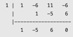
The quotient is:
x² − 5x + 6
Step 3: Factor the Quadratic
x² − 5x + 6 = (x − 2)(x − 3)
Therefore:
(x − 1)(x − 2)(x − 3) = 0
Final Answer
x = 1, 2, or 3

Solving Cubic Equations Using Special Products
Some cubic expressions can be factored using the sum or difference of cubes.
Difference of Cubes
a³ − b³ = (a − b)(a² + ab + b²)
Sum of Cubes
a³ + b³ = (a + b)(a² − ab + b²)
Worked Example: Difference of Cubes
Solve:
x³ − 27 = 0
Recognise:
27 = 3³
Factor:
(x − 3)(x² + 3x + 9) = 0
The first factor gives:
x = 3
For the quadratic:
x² + 3x + 9 = 0
Calculate the discriminant:
Δ = 3² − 4(1)(9)
= 9 − 36
= −27
The quadratic has no real roots.
Final Answer
The only real solution is x = 3.
Worked Example: Sum of Cubes
Solve:
8x³ + 125 = 0
Recognise:
8x³ = (2x)³
125 = 5³
Factor:
(2x + 5)(4x² − 10x + 25) = 0
The first factor gives:
2x + 5 = 0
x = −5/2
The quadratic factor has discriminant:
Δ = (−10)² − 4(4)(25)
= 100 − 400
= −300
Therefore, it has no real roots.
The only real solution is x = −5/2.
Solving Quartic Equations
A quartic equation is a polynomial equation of degree 4.
Quartic equations can have up to four distinct real roots.
Some quartic equations can be solved by factoring directly, while others require substitution or grouping.
Worked Example: Difference of Squares
Solve:
x⁴ − 16 = 0
Recognise:
x⁴ = (x²)²
16 = 4²
Factor:
(x² − 4)(x² + 4) = 0
Factor the first expression:
(x − 2)(x + 2)(x² + 4) = 0
Set each factor equal to zero.
From the linear factors:
x = 2 or x = −2
From:
x² + 4 = 0
we obtain:
x² = −4
This has no real solutions.
Final Answer
x = −2 or x = 2
Although the polynomial has degree 4, it has only two distinct real roots.
Solving Biquadratic Equations
A biquadratic equation is a quartic equation containing powers of x⁴, x², and a constant.
It has the form:
ax⁴ + bx² + c = 0
These equations can often be solved using substitution.
Let:
u = x²
Then:
x⁴ = u²
The quartic becomes a quadratic equation in u.
Worked Example
Solve:
x⁴ − 5x² + 4 = 0
Step 1: Substitute
Let:
u = x²
Then:
u² − 5u + 4 = 0
Step 2: Factor
(u − 1)(u − 4) = 0
Therefore:
u = 1 or u = 4
Step 3: Substitute Back
Since u = x²:
x² = 1
or:
x² = 4
Step 4: Solve
x = ±1
or:
x = ±2
Final Answer
x = −2, −1, 1, or 2
Verification
Substitute x = 2:
2⁴ − 5(2²) + 4
= 16 − 20 + 4
= 0
Substitute x = 1:
1 − 5 + 4 = 0
Because the equation contains only even powers of x, the corresponding negative values also satisfy it.
Biquadratic Equations with No Real Solutions
Not every biquadratic equation has real roots.
Worked Example
Solve:
x⁴ + 5x² + 4 = 0
Let:
u = x²
Then:
u² + 5u + 4 = 0
Factor:
(u + 1)(u + 4) = 0
Therefore:
u = −1 or u = −4
Substitute back:
x² = −1
or:
x² = −4
Neither equation has real solutions.
Final Answer
There are no real solutions.
Important Observation
Because x² ≥ 0 for all real x, a negative value of u cannot produce a real value of x.
This restriction must be considered when using substitution.
Quartic Equations with Repeated Roots
Some quartic equations contain repeated factors.
Worked Example
Solve:
x⁴ − 6x² + 9 = 0
Recognise the perfect square:
(x² − 3)² = 0
Therefore:
x² − 3 = 0
x² = 3
Final Answer
x = ±√3
Each root has multiplicity 2 because:
(x² − 3)² = (x − √3)²(x + √3)²
There are two distinct real roots, each repeated twice.
Solving Quartic Equations by Grouping
Some quartic equations can be factored by grouping or by recognising a common polynomial factor.
Worked Example
Solve:
x⁴ + 2x³ − 9x² − 18x = 0
Step 1: Factor Out x
x(x³ + 2x² − 9x − 18) = 0
Step 2: Group the Cubic
x[(x³ + 2x²) + (−9x − 18)] = 0
Step 3: Factor Each Group
x[x²(x + 2) − 9(x + 2)] = 0
Step 4: Factor the Common Binomial
x(x + 2)(x² − 9) = 0
Step 5: Factor the Difference of Squares
x(x + 2)(x − 3)(x + 3) = 0
Final Answer
x = −3, −2, 0, or 3
The quartic has four distinct real roots.
Understanding Multiple and Repeated Roots
A polynomial can have several different roots, and some roots may appear more than once.
The multiplicity of a root is the number of times its corresponding linear factor appears.
Example
Consider:
P(x) = (x − 2)²(x + 1)³
The roots are:
x = 2, multiplicity 2
x = −1, multiplicity 3
The polynomial has degree:
2 + 3 = 5
However, it has only two distinct real roots.
Types of Multiplicity
|
Multiplicity |
Name |
Typical graph behaviour |
|---|---|---|
|
1 |
Simple root |
Crosses the x-axis |
|
2 |
Double root |
Touches and turns around |
|
3 |
Triple root |
Crosses with flattening |
|
4 |
Quadruple root |
Touches with greater flattening |
|
5 |
Quintuple root |
Crosses with greater flattening |
Important Principle
For a polynomial with real coefficients:
-
Odd-multiplicity roots cause the graph to cross the x-axis.
-
Even-multiplicity roots cause the graph to touch the x-axis without crossing.

Identifying the Number of Possible Solutions
The degree of a polynomial determines the maximum number of distinct real roots.
However, additional information can help us determine how many real roots are possible.
Odd-Degree Polynomials
A polynomial of odd degree with real coefficients must have at least one real root.
Examples:
-
Cubic: at least one distinct real root.
-
Quintic: at least one distinct real root.
-
Seventh-degree: at least one distinct real root.
This occurs because the graph extends in opposite vertical directions as x approaches positive and negative infinity.
Even-Degree Polynomials
An even-degree polynomial may have:
-
No real roots.
-
One or more distinct real roots.
-
Up to as many distinct real roots as its degree.
Example
Consider:
P(x) = x⁴ + 1
For every real x:
x⁴ ≥ 0
Therefore:
x⁴ + 1 > 0
The equation:
x⁴ + 1 = 0
has no real solutions.
Another Example
Consider:
P(x) = (x − 2)⁴
The equation:
(x − 2)⁴ = 0
has only one distinct real root:
x = 2
Its multiplicity is 4.
The Fundamental Theorem of Algebra
The Fundamental Theorem of Algebra states that every nonconstant polynomial of degree n has exactly n complex roots when multiplicities are counted.
For example:
P(x) = x⁴ − 16
Factor:
(x − 2)(x + 2)(x² + 4)
The real roots are:
x = 2 and x = −2
The remaining roots come from:
x² + 4 = 0
x² = −4
Therefore:
x = 2i or x = −2i
The four complex roots are:
−2, 2, −2i, 2i
This accounts for all four roots of the quartic.
Complex Roots in Conjugate Pairs
For a polynomial with real coefficients, nonreal complex roots occur in conjugate pairs.
For example, if:
2 + 3i
is a root, then:
2 − 3i
must also be a root.
This property is useful when determining the remaining roots of higher-degree polynomials.
Using the Rational Root Theorem
The Rational Root Theorem helps identify possible rational roots of polynomials with integer coefficients.
For:
P(x) = aₙxⁿ + ... + a₁x + a₀
a rational root p/q, written in lowest terms, must satisfy:
-
p is a factor of the constant term.
-
q is a factor of the leading coefficient.
Worked Example
Solve:
2x³ − 3x² − 8x + 12 = 0
The constant term is 12.
The leading coefficient is 2.
Possible rational roots include:
±1/2, ±1, ±3/2, ±2, ±3, ±4, ±6, ±12
Step 1: Test x = 2
P(2) = 2(8) − 3(4) − 8(2) + 12
= 16 − 12 − 16 + 12
= 0
Therefore, x − 2 is a factor.
Step 2: Synthetic Division
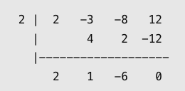
The quotient is:
2x² + x − 6
Step 3: Factor
2x² + x − 6 = (2x − 3)(x + 2)
Therefore:
(x − 2)(2x − 3)(x + 2) = 0
Final Answer
x = −2, 3/2, or 2
Using Synthetic Division to Solve Quartic Equations
Synthetic division can reduce a quartic equation to a cubic equation.
Repeated division can then reduce it further.
Worked Example
Solve:
x⁴ − 5x³ + 5x² + 5x − 6 = 0
Step 1: Test x = 1
P(1) = 1 − 5 + 5 + 5 − 6
= 0
Therefore, x − 1 is a factor.
Step 2: Synthetic Division
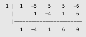
The quotient is:
x³ − 4x² + x + 6
Step 3: Factor the Cubic
Test x = 2:
8 − 16 + 2 + 6 = 0
Therefore, x − 2 is a factor.
Synthetic division:
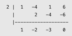
The quotient is:
x² − 2x − 3
Factor:
(x − 3)(x + 1)
Final Factorization
(x − 1)(x − 2)(x − 3)(x + 1) = 0
Final Answer
x = −1, 1, 2, or 3
Solving Equations with Substitution
Some higher-degree equations have repeated exponent patterns.
These can often be simplified by substitution.
Worked Example
Solve:
x⁶ − 7x³ + 6 = 0
Notice that:
x⁶ = (x³)²
Let:
u = x³
Then:
u² − 7u + 6 = 0
Factor:
(u − 1)(u − 6) = 0
Therefore:
u = 1 or u = 6
Substitute back:
x³ = 1
or:
x³ = 6
Final Answer
x = 1 or x = ∛6
Both are real solutions.
Important Observation
Substitution is especially useful when the exponents follow a pattern such as:
-
x⁴ and x²
-
x⁶ and x³
-
x⁸ and x⁴
The goal is to transform a higher-degree equation into a simpler quadratic equation.
Solving Equations with Repeated Factors
Worked Example
Solve:
x⁵ − 6x⁴ + 9x³ = 0
Step 1: Factor Out the GCF
x³(x² − 6x + 9) = 0
Step 2: Factor the Quadratic
x² − 6x + 9 = (x − 3)²
Therefore:
x³(x − 3)² = 0
Step 3: Solve
x³ = 0
or:
(x − 3)² = 0
Therefore:
x = 0 or x = 3
Multiplicities
-
x = 0 has multiplicity 3.
-
x = 3 has multiplicity 2.
There are two distinct real solutions, but five roots when multiplicities are counted.
Interpreting Polynomial Graphs
The graph of a polynomial function provides useful information about its roots.
A root occurs wherever the graph meets the x-axis.
Cubic Functions
A cubic function can have:
-
One distinct real root.
-
Two distinct real roots, with one repeated.
-
Three distinct real roots.
Quartic Functions
A quartic function can have:
-
No real roots.
-
One distinct real root.
-
Two distinct real roots.
-
Three distinct real roots.
-
Four distinct real roots.
Example
Consider:
P(x) = (x + 2)(x − 1)²(x − 3)
The roots are:
x = −2
x = 1
x = 3
The root x = 1 has multiplicity 2.
Therefore:
-
The graph crosses the x-axis at x = −2.
-
The graph touches the x-axis at x = 1.
-
The graph crosses the x-axis at x = 3.

End Behaviour of Higher-Degree Polynomials
The degree and leading coefficient determine the end behaviour of a polynomial.
Even Degree with Positive Leading Coefficient
Both ends of the graph rise.
Example:
y = x⁴
Even Degree with Negative Leading Coefficient
Both ends fall.
Example:
y = −x⁴
Odd Degree with Positive Leading Coefficient
The left end falls and the right end rises.
Example:
y = x³
Odd Degree with Negative Leading Coefficient
The left end rises and the right end falls.
Example:
y = −x³
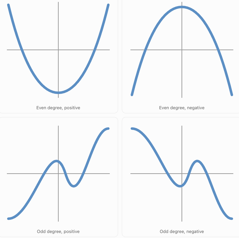
Why End Behaviour Matters
End behaviour helps us:
-
Predict the general shape of polynomial graphs.
-
Determine whether the ends rise or fall.
-
Understand why odd-degree polynomials have at least one real root.
-
Check whether a graph is consistent with its equation.
Real-World Application: Designing a Rectangular Container
A rectangular container has a square base.
Its height is 3 cm greater than the side length of the base.
The container has a volume of 100 cm³.
Find its dimensions.
Step 1: Define the Variable
Let x represent the side length of the square base.
Then:
Length = x
Width = x
Height = x + 3
Step 2: Write the Volume Equation
Volume = Length × Width × Height
Therefore:
x²(x + 3) = 100
Expand:
x³ + 3x² = 100
Rearrange:
x³ + 3x² − 100 = 0
Step 3: Test Possible Roots
Try x = 4:
4³ + 3(4²) − 100
= 64 + 48 − 100
= 12
So x = 4 is not a root.
Try x = 5:
125 + 75 − 100 = 100
So x = 5 is not a root.
There is no simple integer root between 4 and 5.
Step 4: Approximate the Solution
Numerical calculation gives:
x ≈ 3.98 cm
More precisely, x ≈ 3.982.
Step 5: Interpret
The dimensions are approximately:
Length = 3.98 cm
Width = 3.98 cm
Height = 6.98 cm
These values give a volume close to 100 cm³.
Important Lesson
Not every higher-degree polynomial equation can be solved by simple factoring.
When factoring does not produce convenient roots, graphical or numerical methods may be necessary.

Real-World Application: Projectile Motion
A projectile's height is modelled by:
h(t) = −5t³ + 20t² + 25t
where h is measured in metres and t in seconds.
Determine when the projectile is at ground level.
Step 1: Set Height Equal to Zero
−5t³ + 20t² + 25t = 0
Step 2: Factor Out the GCF
−5t(t² − 4t − 5) = 0
Step 3: Factor the Quadratic
t² − 4t − 5 = (t − 5)(t + 1)
Therefore:
−5t(t − 5)(t + 1) = 0
Step 4: Solve
t = 0
t = 5
t = −1
Step 5: Interpret
The negative time is outside the physical interval after launch.
Therefore:
-
t = 0 represents the initial position.
-
t = 5 represents the return to ground level.
The model predicts that the projectile returns to the ground after 5 seconds.
This is an illustrative polynomial model rather than the usual constant-gravity projectile model, which is quadratic.
Real-World Application: Manufacturing and Profit
A manufacturer models profit using:
P(x) = −x³ + 7x² − 14x + 8
where x represents production in thousands of units and P(x) represents profit in thousands of dollars.
The company breaks even when:
P(x) = 0
Step 1: Rearrange and Factor
−x³ + 7x² − 14x + 8 = 0
Multiply by −1:
x³ − 7x² + 14x − 8 = 0
Test x = 1:
1 − 7 + 14 − 8 = 0
Therefore, x − 1 is a factor.
Synthetic division gives:
x² − 6x + 8
Factor:
(x − 2)(x − 4)
Therefore:
(x − 1)(x − 2)(x − 4) = 0
Step 2: Solve
x = 1, 2, or 4
Step 3: Interpret
Because x represents thousands of units, the break-even production levels are:
-
1,000 units.
-
2,000 units.
-
4,000 units.
This illustrates how higher-degree equations can describe several break-even points in a mathematical business model.
Real-World Application: Open-Top Box Design
A rectangular sheet of cardboard measures 20 cm by 14 cm.
Equal squares of side length x are cut from each corner.
The sides are folded upward to create an open-top box.
The resulting dimensions are:
Length = 20 − 2x
Width = 14 − 2x
Height = x
The volume is:
V(x) = x(20 − 2x)(14 − 2x)

Expanding the Volume
First multiply:
(20 − 2x)(14 − 2x)
= 280 − 40x − 28x + 4x²
= 280 − 68x + 4x²
Multiply by x:
V(x) = 4x³ − 68x² + 280x
Suppose the required volume is 288 cm³.
Set:
4x³ − 68x² + 280x = 288
Rearrange:
4x³ − 68x² + 280x − 288 = 0
Divide by 4:
x³ − 17x² + 70x − 72 = 0
Test x = 2:
8 − 68 + 140 − 72
= 8
So x = 2 is not a root.
Test x = 3:
27 − 153 + 210 − 72
= 12
So x = 3 is not a root.
Test x = 4:
64 − 272 + 280 − 72
= 0
Therefore, x − 4 is a factor.
Synthetic division gives:
x² − 13x + 18
The remaining quadratic has solutions:
x = (13 ± √97)/2
Approximately:
x ≈ 1.576
or:
x ≈ 11.424
Physical Restrictions
For the box to exist:
x > 0
20 − 2x > 0
14 − 2x > 0
Therefore:
0 < x < 7
The solution x ≈ 11.424 is invalid because it would produce negative dimensions.
The physically valid solutions are:
x = 4 cm or x ≈ 1.576 cm
Both cut sizes produce a box with volume 288 cm³.
This example demonstrates why solving higher-degree equations requires both algebraic work and interpretation.
Common Mistakes
Forgetting to set the equation equal to zero
The zero product property applies only when a product equals zero.
Stopping before factoring completely
For example:
x³ − 9x = 0
must be factored as:
x(x − 3)(x + 3) = 0
Losing the solution x = 0
Dividing by x can remove a valid solution.
Ignoring repeated roots
The equation:
(x − 2)³ = 0
has one distinct root, x = 2, with multiplicity 3.
Assuming every polynomial has as many distinct real roots as its degree
A quartic may have fewer than four distinct real roots.
Confusing real and complex roots
The equation x² + 4 = 0 has no real roots but two complex roots.
Forgetting to substitute back after using a new variable
If u = x², solutions for u must be converted back into solutions for x.
Accepting negative values of x²
For real x:
x² ≥ 0
Therefore, x² = −3 has no real solution.
Using the wrong synthetic division value
For x + 3, use −3.
Ignoring contextual restrictions
A mathematically valid root may represent an impossible physical length, negative time, or invalid production quantity.
Key Terms
-
Higher-Degree Polynomial: Polynomial with degree greater than 2.
-
Cubic Polynomial: Polynomial of degree 3.
-
Quartic Polynomial: Polynomial of degree 4.
-
Quintic Polynomial: Polynomial of degree 5.
-
Degree: Highest exponent in a nonzero polynomial.
-
Root: Value that satisfies a polynomial equation.
-
Zero: Input value that makes a polynomial function equal zero.
-
Real Root: Root belonging to the real number system.
-
Complex Root: Root belonging to the complex number system.
-
Distinct Roots: Different values that satisfy the equation.
-
Repeated Root: Root that occurs more than once in the factorization.
-
Multiplicity: Number of times a root appears as a factor.
-
Zero Product Property: If a product equals zero, at least one factor equals zero.
-
Greatest Common Factor: Largest factor shared by all terms.
-
Factoring by Grouping: Method of factoring terms in groups.
-
Difference of Squares: Expression of the form a² − b².
-
Sum of Cubes: Expression of the form a³ + b³.
-
Difference of Cubes: Expression of the form a³ − b³.
-
Biquadratic Equation: Quartic equation involving x⁴, x², and a constant.
-
Substitution: Replacing an expression with a new variable to simplify an equation.
-
Factor Theorem: x − a is a factor of P(x) if and only if P(a) = 0.
-
Rational Root Theorem: Theorem identifying possible rational roots of integer-coefficient polynomials.
-
Synthetic Division: Efficient method for dividing by suitable linear factors.
-
Fundamental Theorem of Algebra: Every degree-n nonconstant polynomial has n complex roots, counting multiplicity.
-
Discriminant: Expression used to determine the nature of quadratic roots.
-
End Behaviour: Behaviour of a polynomial graph as x approaches positive or negative infinity.
-
Verification: Checking a proposed solution by substitution.
-
Contextual Restriction: Condition limiting which mathematical solutions are meaningful in a real-world problem.
Key Takeaways
-
Higher-degree polynomial equations have degree 3 or greater.
-
Cubic equations have degree 3 and quartic equations have degree 4.
-
The degree determines the maximum number of distinct real roots.
-
A degree-n polynomial has exactly n complex roots when multiplicities are counted.
-
Odd-degree polynomials with real coefficients always have at least one real root.
-
Even-degree polynomials may have no real roots.
-
Factoring is one of the most effective methods for solving higher-degree polynomial equations.
-
Always check for a greatest common factor first.
-
Grouping and special-product identities can simplify cubic and quartic equations.
-
Synthetic division and the Factor Theorem help find factors of higher-degree polynomials.
-
Biquadratic equations can often be solved by substituting u = x².
-
Repeated roots affect how graphs behave at x-intercepts.
-
Even-multiplicity roots touch the x-axis, while odd-multiplicity roots cross it.
-
Some polynomial equations require numerical or graphical methods.
-
Real-world problems may impose restrictions that eliminate mathematically valid solutions.
-
Every proposed solution should be verified by substitution.
Check Your Understanding
Solve each equation. Give all distinct real solutions unless otherwise stated.
Cubic Equations
-
x³ − 4x = 0
-
x³ − 9x = 0
-
x³ + 3x² − 4x − 12 = 0
-
x³ − 6x² + 11x − 6 = 0
Quartic Equations
-
x⁴ − 16 = 0
-
x⁴ − 5x² + 4 = 0
-
x⁴ − 10x² + 9 = 0
-
x⁴ + 5x² + 4 = 0
Repeated Roots
-
(x − 2)²(x + 3) = 0
-
(x + 1)³(x − 4)² = 0
-
x⁴ − 6x² + 9 = 0
-
x⁵ − 6x⁴ + 9x³ = 0
Higher-Degree Methods
-
x⁶ − 7x³ + 6 = 0
-
x⁶ − 9x⁴ = 0
-
x³ − 27 = 0
-
8x³ + 125 = 0
Reasoning and Applications
-
How many complex roots does a quartic polynomial have when multiplicities are counted?
-
Explain why a cubic polynomial with real coefficients must have at least one real root.
-
A box has a square base of side x and height x + 3. Write an equation for a volume of 100 cm³.
-
Explain why some mathematical roots must be rejected in real-world problems.
Answer Key
|
Question |
Answer |
|---|---|
|
1 |
x = −2, 0, 2 |
|
2 |
x = −3, 0, 3 |
|
3 |
x = −3, −2, 2 |
|
4 |
x = 1, 2, 3 |
|
5 |
x = −2, 2 |
|
6 |
x = −2, −1, 1, 2 |
|
7 |
x = −3, −1, 1, 3 |
|
8 |
No real solutions |
|
9 |
x = 2 (multiplicity 2), −3 |
|
10 |
x = −1 (multiplicity 3), 4 (multiplicity 2) |
|
11 |
x = ±√3, each multiplicity 2 |
|
12 |
x = 0 (multiplicity 3), 3 (multiplicity 2) |
|
13 |
x = 1, ∛6 |
|
14 |
x = −3, 0, 3 |
|
15 |
x = 3 |
|
16 |
x = −5/2 |
|
17 |
Four |
|
18 |
Its graph has opposite end behaviour and must cross the x-axis |
|
19 |
x²(x + 3) = 100 |
|
20 |
Some roots may violate physical restrictions such as positive lengths or nonnegative time |
Extended Challenge
Cubic Equations
-
x³ − 16x = 0
-
2x³ − 8x² + 6x = 0
-
x³ − 4x² − 9x + 36 = 0
-
x³ + 2x² − 5x − 6 = 0
-
3x³ − 12x² + 9x = 0
Quartic Equations
-
x⁴ − 13x² + 36 = 0
-
x⁴ − 25 = 0
-
x⁴ − 8x² + 16 = 0
-
x⁴ + 2x³ − 9x² − 18x = 0
-
x⁴ − 5x³ + 5x² + 5x − 6 = 0
Higher-Degree Substitution
-
x⁶ − 10x³ + 9 = 0
-
x⁸ − 17x⁴ + 16 = 0
-
x⁶ − 5x⁴ + 4x² = 0
-
x⁶ + 5x³ + 4 = 0
-
x⁸ − 81 = 0
Roots and Multiplicity
-
Construct a quartic equation with roots x = −2 and x = 3, each with multiplicity 2.
-
Construct a fifth-degree polynomial with roots x = 1 (multiplicity 3) and x = −4 (multiplicity 2).
-
Explain why a fourth-degree polynomial may have only one distinct real root.
-
Determine the roots and multiplicities of (x² − 9)² = 0.
-
Sketch the general behaviour of y = (x + 2)²(x − 1)³.
Real-World Applications
-
A container has a square base and height 2 cm greater than its side length. Its volume is 48 cm³. Form and solve the cubic equation for its dimensions.
-
A manufacturer's profit is P(x) = −x³ + 6x² − 11x + 6. Determine the break-even production levels.
-
A rectangular prism has dimensions x, x + 1, and x + 2. Its volume is 60 cm³. Determine its dimensions.
-
An open-top box is formed by cutting equal squares from the corners of a rectangular sheet. Derive a cubic expression for its volume.
-
Explain why a higher-degree equation may require numerical methods even when factoring is the preferred first strategy.
Final Challenge: Investigating a Quartic Polynomial
Consider:
P(x) = x⁴ − 5x³ + 5x² + 5x − 6
Complete the investigation.
-
Identify the degree of the polynomial.
-
State the maximum number of distinct real roots.
-
List possible rational roots using the Rational Root Theorem.
-
Test x = 1 using the Factor Theorem.
-
Determine whether x − 1 is a factor.
-
Use synthetic division to divide P(x) by x − 1.
-
Write the resulting cubic polynomial.
-
Test another possible rational root.
-
Use synthetic division again.
-
Factor the remaining quadratic.
-
Write P(x) in completely factored form.
-
Identify all real roots.
-
State the multiplicity of each root.
-
Verify each root by substitution.
-
Determine the x-intercepts of the graph.
-
Describe the end behaviour of the polynomial.
-
Predict whether the graph crosses or touches the x-axis at each root.
-
Sketch the general graph.
-
Explain how the Factor Theorem and synthetic division simplify higher-degree equations.
-
Summarise the relationship between polynomial degree, roots, multiplicity, and graph behaviour.
Further Investigation: Constructing a Polynomial
Create a polynomial equation that satisfies these conditions:
-
It has degree 6.
-
It has a root at x = −3 with multiplicity 2.
-
It has a root at x = 1 with multiplicity 3.
-
It has a root at x = 4 with multiplicity 1.
Then:
-
Write the polynomial in factored form.
-
Determine its degree.
-
Identify all distinct real roots.
-
State the multiplicity of each root.
-
Predict how the graph behaves at each root.
-
Determine the end behaviour if the leading coefficient is positive.
-
Expand the polynomial into standard form.
-
Verify the roots by substitution.
-
Explain why the polynomial has fewer distinct real roots than its degree.
-
Investigate how changing the multiplicity of one root affects the graph.