Applications of Sequences and Series

Introduction

Many events in the world occur repeatedly. A pendulum swings back and forth, a wheel completes rotations, a machine produces items in cycles, and a bouncing ball repeatedly rises and falls. Even when motion appears complicated, mathematical patterns can help us describe and predict what happens.

Consider a car travelling at a constant speed of 15 metres per second.

After one second, it has travelled 15 metres. After two seconds, it has travelled 30 metres. After three seconds, it has travelled 45 metres.

The distances form the sequence:

0, 15, 30, 45, 60, 75, ...

This is an arithmetic sequence because the distance increases by the same amount during every second.

Now consider a bouncing ball that reaches 80% of its previous maximum height after every bounce.

If its first maximum height is 2 metres, the following heights are:

2, 1.6, 1.28, 1.024, 0.8192, ...

This is a geometric sequence because each height is multiplied by 0.8.

Both situations involve motion, but they follow different mathematical patterns.

By identifying these patterns, we can construct mathematical models, calculate future values, and explain how repeated physical processes behave.

In this lesson, we will explore connections between sequences, motion, repeated events, physics, engineering, and technology.

Understanding Repeated Processes

A repeated process is an event or action that occurs more than once according to a recognisable rule.

Repeated processes may involve:

• Equal changes during each time interval

• Repeated multiplication by a constant

• Cycles that repeat after fixed intervals

• Changes that depend on previous values

• Repeated movements or mechanical operations

• Accumulation of distance, energy, or material

• Gradual decreases caused by friction or energy losses

Mathematical sequences are useful because they describe quantities at separate stages of a process.

For example, a machine that produces 12 components every minute creates the cumulative production sequence:

12, 24, 36, 48, 60, ...

A rotating wheel completing five revolutions every second produces:

5, 10, 15, 20, 25, ...

Both sequences increase by a constant amount.

However, not every repeated process produces an arithmetic sequence. The mathematical model depends on how the quantity changes.

Discrete and Continuous Models

Motion usually occurs continuously, but we often record measurements at regular intervals.

For example, a car's position may be recorded every second.

These measurements form a discrete sequence.

The underlying motion may be described by a continuous function:

x(t) = 10t

where:

• x is position in metres.

• t is time in seconds.

At whole-number times, the function generates the sequence:

0, 10, 20, 30, 40, ...

This connection between continuous functions and discrete sequences is important in physics, engineering, and computer simulations.

A sequence model describes selected time steps, while a continuous model describes the quantity at every time within its domain.

Constant Velocity and Arithmetic Sequences

An object moving at constant velocity travels equal displacements during equal time intervals.

For motion in a straight line:

Displacement = Velocity × Time

or:

Δx = vt

If the initial position is x₀, the position after time t is:

x = x₀ + vt

When positions are measured at equal time intervals Δt, the sequence follows:

xₙ = x₀ + nvΔt

This is an arithmetic sequence because the difference between consecutive positions is constant.

Worked Example 1: A Train Moving at Constant Velocity

A train begins at position 200 m and travels east at 25 m/s.

Find its position every two seconds for the first ten seconds.

Step 1: Identify the values.

Initial position:

x₀ = 200 m

Velocity:

v = 25 m/s

Time interval:

Δt = 2 s

Step 2: Calculate the displacement during each interval.

Δx = vΔt

= 25 × 2

= 50 m

Step 3: Write the sequence.

200, 250, 300, 350, 400, 450

Step 4: Write an explicit rule.

xₙ = 200 + 50n

where n is the number of two-second intervals.

Step 5: Verify.

After five intervals:

x₅ = 200 + 50(5)

= 450 m

Answer: The train is at position 450 m after ten seconds.

Visualising constant velocity

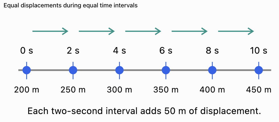
The equal spacing illustrates the constant difference between consecutive terms.

Acceleration and Quadratic Patterns

Not all objects move at constant velocity.

When an object accelerates, its velocity changes over time.

For constant acceleration:

v = u + at

where:

• v = final velocity

• u = initial velocity

• a = acceleration

• t = time

The displacement from the initial position is:

s = ut + ½at²

The term t² creates a quadratic relationship between displacement and time.

Worked Example 2: Motion from Rest

A car starts from rest and accelerates uniformly at 2 m/s².

Calculate its displacement after each of the first five seconds.

Given:

u = 0

a = 2 m/s²

Use:

s = ut + ½at²

Since u = 0:

s = ½(2)t²

s = t²

Calculate:

The sequence is:

0, 1, 4, 9, 16, 25, ...

These are square numbers.

The first differences are:

1, 3, 5, 7, 9

The second differences are:

2, 2, 2, 2

This shows that uniformly accelerated motion produces a quadratic position sequence when measured at equally spaced times.

Why do the differences increase?

The car's velocity increases by 2 m/s every second.

Therefore, it travels a greater distance during each successive second.

The sequence of distances travelled during individual seconds is:

1, 3, 5, 7, 9, ...

This is an arithmetic sequence of odd numbers.

The total displacement is the sum of these distances.

Thus:

1 + 3 + 5 + ... + (2n − 1) = n²

This connects motion, arithmetic sequences, square numbers, and algebra.

Visualising quadratic displacement

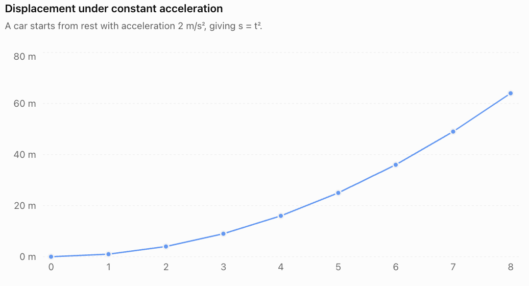
The upward-curving graph shows that displacement increases more rapidly as time passes.

Velocity as an Arithmetic Sequence

For constant acceleration:

v = u + at

At equal time intervals, the velocity increases or decreases by a constant amount.

Worked Example 3: Velocity of an Accelerating Object

A cyclist begins at 4 m/s and accelerates at 1.5 m/s².

Find the velocity after each of the first five seconds.

Use:

v = 4 + 1.5t

The velocity sequence is:

4, 5.5, 7, 8.5, 10, 11.5, ...

This is an arithmetic sequence with common difference 1.5.

The recursive rule is:

vₙ₊₁ = vₙ + 1.5

The explicit rule is:

vₙ = 4 + 1.5n

where n represents elapsed seconds.

This demonstrates an important distinction:

• Velocity under constant acceleration follows an arithmetic sequence.

• Position under constant acceleration follows a quadratic sequence.

Repeated Motion and Geometric Sequences

Some repeated processes involve multiplying a quantity by the same factor after each event.

A bouncing ball provides a useful example.

When a ball strikes the ground, some mechanical energy is dissipated through sound, heating, and deformation.

As a result, the ball generally rebounds to a lower height.

A simplified model assumes that each rebound reaches a fixed fraction of the previous maximum height.

If the rebound factor is r, then:

hₙ = h₀rⁿ

where:

• h₀ = initial height

• hₙ = height after n rebounds

• r = rebound-height ratio, with 0 ≤ r < 1

Worked Example 4: Bouncing Ball

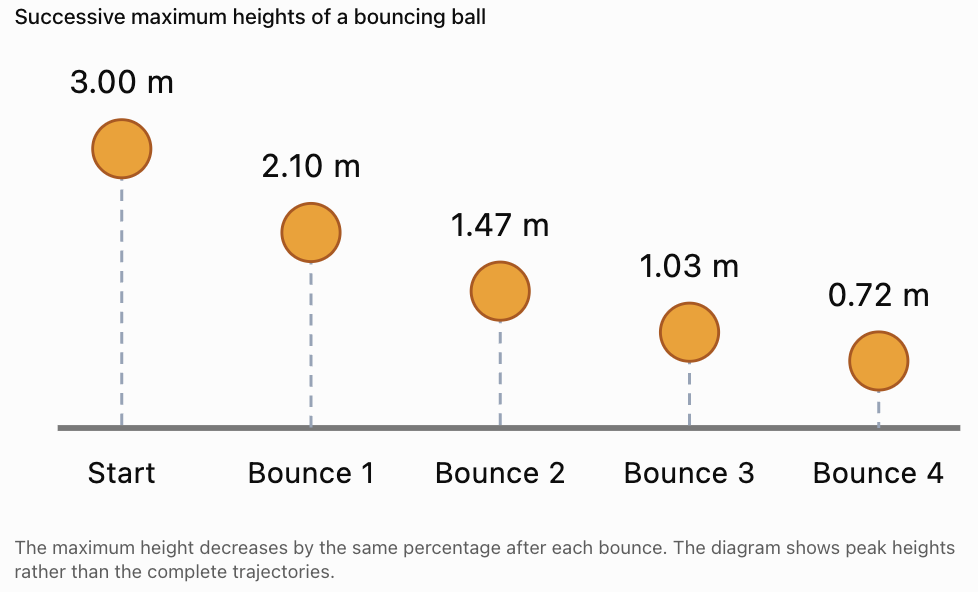
A ball is dropped from a height of 3 m.

After each bounce, it reaches 70% of its previous maximum height.

Calculate the first four rebound heights.

Initial height:

h₀ = 3 m

Rebound factor:

r = 0.70

First bounce

h₁ = 3(0.70)

= 2.10 m

Second bounce

h₂ = 3(0.70)²

= 1.47 m

Third bounce

h₃ = 3(0.70)³

= 1.029 m

Fourth bounce

h₄ = 3(0.70)⁴

= 0.7203 m

The sequence is:

3, 2.1, 1.47, 1.029, 0.7203, ...

This is a geometric sequence with common ratio 0.70.

Visualising successive bounces

Total Distance Travelled by a Bouncing Ball

Geometric sequences can also help calculate the total distance travelled during repeated bouncing.

Suppose a ball is dropped from height H and rebounds to a constant fraction r of its previous height.

The ball first travels downward through distance H.

After the first bounce, it travels upward through distance Hr and downward through another Hr.

After the second bounce, it travels upward through Hr² and downward through Hr².

The total distance is:

D = H + 2Hr + 2Hr² + 2Hr³ + ...

The geometric series is:

r + r² + r³ + ... = r/(1 − r)

for 0 ≤ r < 1.

Therefore:

D = H + 2Hr/(1 − r)

This is the total distance predicted by the idealised model over infinitely many bounces.

Worked Example 5: Total Bouncing Distance

A ball is dropped from 2 m and rebounds to 60% of its previous maximum height.

Find the total distance travelled in the idealised infinite-bounce model.

Given:

H = 2

r = 0.60

Use:

D = H + 2Hr/(1 − r)

D = 2 + [2(2)(0.60)]/(1 − 0.60)

= 2 + 2.4/0.4

= 2 + 6

Answer: 8 m

This result assumes the same rebound-height ratio for every bounce. Real balls eventually stop bouncing, and the ratio may change.

Periodic Motion and Repeating Cycles

A periodic process repeats after a fixed interval.

Examples include:

• Pendulum oscillations

• Wheel rotations

• Vibrations of a spring

• Alternating electrical signals

• Rotating machinery

• Repeating mechanical cycles

Two important quantities are:

Period (T): Time required for one complete cycle.

Frequency (f): Number of cycles completed per second.

Their relationship is:

f = 1/T

or:

T = 1/f

Frequency is measured in hertz (Hz).

Worked Example 6: Pendulum Oscillations

A pendulum completes one oscillation every 2.5 seconds.

Calculate:

a) Its frequency.

b) The number of complete oscillations in 60 seconds.

Part a: Frequency

f = 1/T

= 1/2.5

f = 0.4 Hz

Part b: Number of oscillations

Number of cycles = Time/Period

= 60/2.5

Answer: 24 complete oscillations

The completion times form an arithmetic sequence:

2.5, 5.0, 7.5, 10.0, 12.5, ...

The nth completion time is:

tₙ = 2.5n

This illustrates how periodic motion can be represented using arithmetic sequences.

Rotational Motion and Repeated Events

Rotating objects are particularly suitable for sequence models.

Examples include:

• Wheels

• Gears

• Turbines

• Fans

• Motors

• Conveyor rollers

If a wheel rotates at a constant rate, the total number of completed revolutions increases linearly with time.

Worked Example 7: Wheel Revolutions

A wheel completes 12 revolutions every second.

Calculate:

a) The number of revolutions after 5 seconds.

b) The number of revolutions after 20 seconds.

c) The general rule for the number of revolutions after t seconds.

Part a

N = 12 × 5

N = 60 revolutions

Part b

N = 12 × 20

N = 240 revolutions

Part c

N(t) = 12t

At whole-second intervals, the sequence is:

12, 24, 36, 48, 60, ...

This is an arithmetic sequence.

Connecting rotations to distance

If a wheel rolls without slipping, the distance travelled during one complete revolution equals its circumference.

Circumference:

C = 2πr

If a wheel has radius 0.35 m:

C = 2π(0.35)

= 0.7π m

After 100 revolutions:

Distance = 100(0.7π)

= 70π m

Distance ≈ 219.91 m

This connects sequences, circular geometry, and motion.

Recursive Models in Motion

A recursive model calculates a new value using a previous value.

In motion, recursive models are useful when velocity, position, or another quantity changes repeatedly.

For example:

vₙ₊₁ = vₙ + aΔt

xₙ₊₁ = xₙ + vₙΔt

These rules form a simple numerical method for modelling motion.

The second rule uses the velocity at the beginning of the time interval, so it is an approximation when the object accelerates.

This method is known as forward Euler integration.

Worked Example 8: Numerical Motion Model

An object begins with:

Initial position = 0 m

Initial velocity = 2 m/s

Acceleration = 1 m/s²

Time step = 1 s

Use:

vₙ₊₁ = vₙ + 1

xₙ₊₁ = xₙ + vₙ

Calculate the first four time steps.

The position sequence is:

0, 2, 5, 9, 14, ...

The first differences are:

2, 3, 4, 5

The second differences are:

1, 1, 1

The position sequence is quadratic.

Comparing the numerical model with exact motion

The exact displacement after four seconds is:

s = ut + ½at²

= 2(4) + ½(1)(4²)

= 8 + 8

s = 16 m

The numerical model predicts 14 m.

The difference occurs because the model uses the velocity at the beginning of each time step and does not account for the increase in velocity within that step.

Smaller time steps generally improve the approximation for this situation.

This is an important example of how mathematical sequences are used in scientific computing.

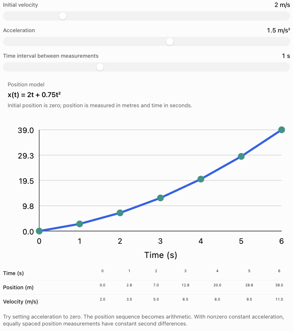
Interactive Motion Sequence Explorer

Explore how the sequence of positions changes when an object moves with different initial velocities and constant accelerations.

Repeated Processes in Technology

Mathematical sequences are widely used in technology because machines and computers frequently perform repeated operations.

1. Manufacturing systems

A machine produces 40 components every minute.

The cumulative number of components after n minutes is:

Cₙ = 40n

This is an arithmetic sequence.

2. Computer simulations

A computer repeatedly updates position and velocity using numerical rules.

For example:

vₙ₊₁ = vₙ + aΔt

xₙ₊₁ = xₙ + vₙΔt

This allows computers to approximate the motion of vehicles, projectiles, and other objects.

3. Mechanical vibrations

Machines may vibrate repeatedly.

If the amplitude decreases by a fixed factor after each cycle, the peak amplitudes may follow a geometric sequence.

4. Automated systems

Robots often perform repeated movements.

If a robotic arm moves 0.25 m during each cycle, its cumulative travel distance after n cycles is:

Dₙ = 0.25n

5. Digital signals

Computers record sound, motion, and other signals at regular time intervals.

These measurements form sequences that can be analysed mathematically.

Damped Oscillations and Geometric Decay

A vibrating system may gradually lose energy because of friction or resistance.

As a result, its amplitude may decrease over time.

A simplified discrete model is:

Aₙ = A₀rⁿ

where:

• A₀ = initial amplitude

• r = amplitude reduction factor

• n = number of completed cycles

Worked Example 9: Damped Vibration

A vibrating system begins with an amplitude of 10 cm.

After each cycle, the amplitude becomes 85% of its previous value.

Calculate the amplitude after six cycles.

Given:

A₀ = 10 cm

r = 0.85

n = 6

Use:

A₆ = 10(0.85)⁶

≈ 10(0.3771495)

Answer: Approximately 3.77 cm

The sequence is:

10, 8.5, 7.225, 6.14125, ...

This is a geometric decay pattern.

Why is this useful?

Damping models are important when studying:

• Vehicle suspension systems

• Building vibrations

• Mechanical springs

• Industrial machinery

• Measuring instruments

• Electronic oscillators

The fixed-ratio model is an approximation. Real damping may depend on velocity, amplitude, and other physical conditions.

Repeated Processes and Cumulative Change

Some processes involve repeatedly adding quantities.

Others involve repeatedly multiplying quantities.

This distinction helps us choose the correct model.

Recognising the type of pattern is often the most important step in constructing a useful model.

Predicting Future Outcomes

Mathematical patterns allow us to predict values beyond the observations already collected.

However, a prediction is only as reliable as the assumptions behind the model.

Worked Example 10: Predicting Future Motion

A vehicle's position is recorded every two seconds.

The positions are:

5, 17, 29, 41, 53, ...

Find its position at the tenth measurement, counting the initial position as the first term.

Step 1: Identify the common difference.

17 − 5 = 12

29 − 17 = 12

The sequence is arithmetic.

Step 2: Write the general formula.

aₙ = a₁ + (n − 1)d

aₙ = 5 + 12(n − 1)

Step 3: Calculate the tenth term.

a₁₀ = 5 + 12(9)

= 5 + 108

Answer: 113 m

Interpreting the result

The vehicle moves 12 m every two seconds.

Therefore, its velocity is:

v = 12/2

v = 6 m/s

The prediction assumes the vehicle continues moving at constant velocity.

If the vehicle accelerates or brakes, the model will no longer accurately describe its position.

Evaluating Motion and Repeated-Process Models

Mathematical models simplify real-world processes.

This makes them useful, but it also creates limitations.

Constant velocity assumptions

A constant-velocity model ignores acceleration, braking, and changes in direction.

Constant acceleration assumptions

A constant-acceleration model assumes acceleration does not change during the time interval.

Real acceleration may vary because of friction, drag, or changing forces.

Energy losses

Bouncing-ball and vibration models may assume a constant reduction factor.

Actual energy losses can change with speed, temperature, and material properties.

Measurement errors

Recorded positions, times, and velocities may contain uncertainty.

Discrete approximations

Numerical models use finite time steps.

Large time steps may produce inaccurate predictions.

Long-term predictions

A model that describes a few cycles accurately may not remain valid indefinitely.

Physical constraints

Mathematical models must respect physical limits.

For example, a bouncing ball cannot continue bouncing indefinitely with perfectly predictable behaviour.

A good mathematical model should be tested against observations and revised when necessary.

Real-World Applications

Common Mistakes

Mistake 1: Assuming every repeated process is arithmetic

Some repeated processes are geometric, quadratic, periodic, or recursive.

Mistake 2: Confusing distance and displacement

Distance measures total path length, while displacement measures the change in position.

Mistake 3: Confusing constant velocity with constant acceleration

Constant velocity means velocity does not change. Constant acceleration means velocity changes at a constant rate.

Mistake 4: Assuming position and velocity follow the same sequence

Under constant acceleration, velocity is arithmetic at equal time intervals, while position is quadratic.

Mistake 5: Using the wrong common ratio

A 20% reduction corresponds to a multiplier of 0.80, not 0.20.

Mistake 6: Confusing period and frequency

Period is time per cycle. Frequency is cycles per second.

Mistake 7: Forgetting the initial value

A recursive model requires a starting position, velocity, amplitude, or other initial quantity.

Mistake 8: Ignoring units

Position, velocity, acceleration, time, and frequency have different units.

Mistake 9: Assuming a numerical approximation is exact

Recursive numerical methods may introduce approximation errors.

Mistake 10: Extending a model beyond realistic conditions

A mathematical rule may no longer describe a physical process after conditions change.

Mistake 11: Confusing cumulative distance with distance per cycle

A sequence of total distances may follow a different pattern from the distances travelled during individual cycles.

Mistake 12: Assuming a prediction is guaranteed

Predictions depend on the accuracy of the model and its assumptions.

Key Terms

• Motion: Change in position over time.

• Repeated Process: Event or action occurring multiple times according to a rule.

• Sequence: Ordered list of values.

• Arithmetic Sequence: Sequence with a constant difference between consecutive terms.

• Geometric Sequence: Sequence with a constant ratio between consecutive terms.

• Quadratic Sequence: Sequence described by a quadratic expression.

• Recursive Rule: Rule calculating a term from previous terms.

• Explicit Formula: Formula calculating a term directly from its position.

• Discrete Model: Model describing values at separate points or time steps.

• Continuous Model: Model describing quantities continuously over an interval.

• Position: Location of an object relative to a reference point.

• Displacement: Change in position.

• Distance: Total length of the path travelled.

• Velocity: Rate of change of displacement.

• Speed: Rate at which distance is travelled.

• Acceleration: Rate of change of velocity.

• Constant Velocity: Motion with unchanged velocity.

• Constant Acceleration: Motion with a constant rate of change of velocity.

• Periodic Motion: Motion that repeats after equal time intervals.

• Period: Time required for one complete cycle.

• Frequency: Number of cycles completed per second.

• Oscillation: Repeated movement around an equilibrium position.

• Amplitude: Maximum displacement from equilibrium.

• Damping: Reduction in oscillation amplitude caused by energy losses.

• Rebound Factor: Ratio between consecutive rebound heights.

• Rotation: Turning movement around an axis.

• Revolution: One complete rotation.

• Circumference: Distance around a circle.

• Numerical Model: Model using numerical calculations to approximate a process.

• Time Step: Interval between successive calculations or measurements.

• Prediction: Estimated future outcome based on a model.

• Extrapolation: Using a model to predict beyond observed values.

• Mathematical Simulation: Computational representation of a process using mathematical rules.

• Model Limitation: Condition restricting the accuracy or usefulness of a model.

Key Takeaways

• Repeated processes occur in motion, engineering, technology, and many natural systems.

• Mathematical sequences describe quantities measured at successive stages.

• Constant velocity produces an arithmetic position sequence at equal time intervals.

• Constant acceleration produces an arithmetic velocity sequence.

• Constant acceleration produces a quadratic position sequence.

• Repeated percentage reductions produce geometric decay sequences.

• Bouncing-ball heights can be modelled using geometric sequences.

• Periodic motion repeats after a fixed time interval.

• Frequency and period are reciprocals.

• Constant-rate rotations can be represented using arithmetic sequences.

• Recursive rules are useful for modelling motion step by step.

• Numerical models approximate continuous motion using discrete calculations.

• Mathematical patterns help predict future positions, velocities, amplitudes, and event counts.

• Real-world models depend on assumptions that must be evaluated.

• Recognising mathematical structures helps connect sequences with physics and technology.

Check Your Understanding

Questions

Question 1: Identifying a Motion Pattern

A vehicle's position is recorded every second:

0, 8, 16, 24, 32, ...

Identify the type of sequence and determine the vehicle's velocity.

Question 2: Constant Velocity

A train begins at position 100 m and moves at 20 m/s.

Find its position after six seconds.

Question 3: Arithmetic Velocity Sequence

A car begins at 5 m/s and accelerates at 2 m/s².

Write the velocity sequence for the first five seconds, including the initial velocity.

Question 4: Quadratic Motion

An object starts from rest and accelerates at 4 m/s².

Calculate its displacement after three seconds.

Question 5: First Differences

The positions of an object are:

0, 2, 8, 18, 32, ...

Find the first and second differences.

What type of sequence is this?

Question 6: Bouncing Ball

A ball is dropped from 4 m and rebounds to 75% of its previous height.

Calculate the maximum height after three bounces.

Question 7: Geometric Decay

A vibrating system begins with an amplitude of 12 cm.

The amplitude decreases by 10% after each cycle.

Calculate the amplitude after five cycles.

Question 8: Pendulum Frequency

A pendulum completes one oscillation every 4 seconds.

Calculate its frequency.

Question 9: Counting Oscillations

A pendulum has a period of 1.5 seconds.

How many complete oscillations does it make in 60 seconds?

Question 10: Wheel Revolutions

A wheel completes 8 revolutions per second.

Calculate the number of revolutions after 25 seconds.

Question 11: Wheel Distance

A wheel has radius 0.4 m.

It rolls without slipping for 50 revolutions.

Calculate the distance travelled.

Question 12: Recursive Motion Model

An object begins with velocity 3 m/s.

Its velocity increases by 2 m/s during every one-second interval.

Write a recursive model and calculate its velocity after five seconds.

Question 13: Numerical Approximation

An object begins at position 0 m with velocity 4 m/s.

Its acceleration is 2 m/s².

Using a one-second time step and the rules:

vₙ₊₁ = vₙ + 2

xₙ₊₁ = xₙ + vₙ

calculate its approximate position after three seconds.

Question 14: Evaluating Models

Explain three limitations of using a fixed rebound factor to model a bouncing ball over many bounces.

Question 15: Integrated Challenge

A car starts from rest and accelerates uniformly at 3 m/s².

a) Write the velocity formula.

b) Calculate the velocity after five seconds.

c) Write the displacement formula.

d) Calculate the displacement after five seconds.

e) Generate the displacement sequence at times 0, 1, 2, 3, 4, and 5 seconds.

f) Explain why the displacement sequence is quadratic.

Fully Worked Answers

Answer 1: Identifying a Motion Pattern

Sequence:

0, 8, 16, 24, 32, ...

Common difference:

8

The sequence is arithmetic.

The position increases by 8 m every second.

Velocity:

v = 8/1

Answer: 8 m/s

Answer 2: Constant Velocity

Initial position:

x₀ = 100 m

Velocity:

v = 20 m/s

Time:

t = 6 s

Use:

x = x₀ + vt

x = 100 + 20(6)

= 100 + 120

Answer: 220 m

Answer 3: Arithmetic Velocity Sequence

Initial velocity:

u = 5 m/s

Acceleration:

a = 2 m/s²

Use:

v = u + at

At t = 0:

v = 5 m/s

At t = 1:

v = 7 m/s

At t = 2:

v = 9 m/s

At t = 3:

v = 11 m/s

At t = 4:

v = 13 m/s

At t = 5:

v = 15 m/s

Sequence: 5, 7, 9, 11, 13, 15

Answer 4: Quadratic Motion

Initial velocity:

u = 0

Acceleration:

a = 4 m/s²

Time:

t = 3 s

Use:

s = ut + ½at²

s = 0 + ½(4)(3²)

= 2(9)

Answer: 18 m

Answer 5: First Differences

Position sequence:

0, 2, 8, 18, 32

First differences:

2, 6, 10, 14

Second differences:

4, 4, 4

Because the second differences are constant, the sequence is quadratic.

Answer: Quadratic sequence

Answer 6: Bouncing Ball

Initial height:

h₀ = 4 m

Rebound factor:

r = 0.75

Number of bounces:

n = 3

Use:

hₙ = h₀rⁿ

h₃ = 4(0.75)³

= 4(0.421875)

Answer: 1.6875 m

Answer 7: Geometric Decay

Initial amplitude:

A₀ = 12 cm

Reduction:

10%

Remaining factor:

r = 0.90

Number of cycles:

n = 5

Use:

Aₙ = A₀rⁿ

A₅ = 12(0.90)⁵

= 12(0.59049)

Answer: Approximately 7.09 cm

Answer 8: Pendulum Frequency

Period:

T = 4 s

Use:

f = 1/T

f = 1/4

Answer: 0.25 Hz

Answer 9: Counting Oscillations

Period:

T = 1.5 s

Time:

t = 60 s

Number of cycles:

N = t/T

N = 60/1.5

Answer: 40 complete oscillations

Answer 10: Wheel Revolutions

Rotation rate:

8 revolutions per second

Time:

25 seconds

Number of revolutions:

N = 8 × 25

Answer: 200 revolutions

Answer 11: Wheel Distance

Radius:

r = 0.4 m

Circumference:

C = 2πr

= 2π(0.4)

= 0.8π m

Number of revolutions:

50

Distance:

D = 50(0.8π)

= 40π

Answer: Approximately 125.66 m

Answer 12: Recursive Motion Model

Initial velocity:

v₀ = 3 m/s

Increase per second:

2 m/s

Recursive rule:

vₙ₊₁ = vₙ + 2

After five seconds:

v₅ = 3 + 5(2)

= 13

Answer: 13 m/s

Answer 13: Numerical Approximation

Initial values:

x₀ = 0 m

v₀ = 4 m/s

Acceleration:

2 m/s²

Time step:

1 s

Rules:

vₙ₊₁ = vₙ + 2

xₙ₊₁ = xₙ + vₙ

First step

x₁ = 0 + 4 = 4

v₁ = 4 + 2 = 6

Second step

x₂ = 4 + 6 = 10

v₂ = 6 + 2 = 8

Third step

x₃ = 10 + 8 = 18

v₃ = 8 + 2 = 10

Answer: Approximate position = 18 m

For comparison, the exact constant-acceleration model gives:

s = 4(3) + ½(2)(3²)

= 12 + 9

= 21 m

The numerical model underestimates the exact displacement by 3 m.

Answer 14: Evaluating Models

Three limitations are:

1. Changing energy losses

The proportion of energy lost during each bounce may change as the ball slows.

2. Surface conditions

The rebound behaviour depends on the material and condition of the ball and surface.

3. Real stopping behaviour

A mathematical geometric sequence predicts smaller and smaller rebounds indefinitely, but a real ball eventually stops bouncing.

Therefore, the fixed-ratio model is useful as an approximation but does not describe every detail of real bouncing motion.

Answer 15: Integrated Challenge

Initial velocity:

u = 0

Acceleration:

a = 3 m/s²

Part a: Velocity formula

v = u + at

Since u = 0:

v = 3t

Part b: Velocity after five seconds

v = 3(5)

Answer: 15 m/s

Part c: Displacement formula

s = ut + ½at²

Since u = 0:

s = ½(3)t²

s = 1.5t²

Part d: Displacement after five seconds

s = 1.5(5²)

= 1.5(25)

Answer: 37.5 m

Part e: Displacement sequence

At t = 0:

s = 0

At t = 1:

s = 1.5

At t = 2:

s = 6

At t = 3:

s = 13.5

At t = 4:

s = 24

At t = 5:

s = 37.5

Sequence: 0, 1.5, 6, 13.5, 24, 37.5

Part f: Explain the quadratic pattern

First differences:

1.5, 4.5, 7.5, 10.5, 13.5

Second differences:

3, 3, 3, 3

Because the second differences are constant, the sequence is quadratic.

This agrees with the displacement formula:

s = 1.5t²

The quadratic pattern occurs because the car's velocity increases at a constant rate, causing it to travel greater distances during successive equal time intervals.

Final Reflection

Motion and repeated processes provide important real-world applications of mathematical sequences.

Constant velocity creates arithmetic position patterns, while constant acceleration produces arithmetic velocity patterns and quadratic position patterns. Bouncing balls and damped vibrations can be represented using geometric decay, while periodic motion creates predictable cycles.

Recursive models extend these ideas by allowing computers and engineers to calculate changing quantities one step at a time.

Recognising the mathematical structure of a repeated process helps us select appropriate formulas, interpret observations, and predict future outcomes.

The most important lesson is that sequences provide a powerful connection between mathematics, physics, and technology. By understanding how quantities change during repeated processes, we can construct models that explain motion, support scientific calculations, and help predict the behaviour of real systems.