Special Sequences and Mathematical Patterns
4. Recursive Models
Learning outcomes
- I can explain how recursive models describe repeated processes.
- I can use recursive rules to model real-world situations.
- I can generate terms in recursive sequences.
- I can interpret recursive models involving population growth or financial situations.
- I can compare recursive and explicit approaches to modeling patterns.
Introduction
Many situations in mathematics and everyday life involve processes that repeat over time.
A bank account earns interest each year. A population changes from one generation to the next. A person saves a fixed amount of money every month. A medicine gradually leaves the bloodstream, while new doses may be added at regular intervals.
In each situation, the next value depends on what happened previously.
These processes can often be described using recursive models.
A recursive model is a mathematical rule that calculates a new value using one or more previous values. Instead of describing a quantity only in terms of time, a recursive model describes how that quantity changes from one step to the next.
Recursive models are especially useful when studying sequences, population growth, compound interest, savings, loans, and other repeated processes.
Understanding recursion helps us recognise patterns, predict future values, and connect mathematical sequences with real-world applications.
What Is a Recursive Model?
A recursive model is a mathematical relationship in which each new value is calculated using an earlier value or values.
For example, consider the sequence:
3, 7, 11, 15, 19, 23, ...
Each term is obtained by adding 4 to the previous term.
We can describe the pattern using:
aₙ = aₙ₋₁ + 4
with the starting value:
a₀ = 3
Here:
-
aₙ represents the value at step n.
-
aₙ₋₁ represents the value at the previous step.
-
4 represents the amount added at every step.
-
a₀ = 3 provides the initial value.
The starting value is called an initial condition.
Without an initial condition, the recursive rule does not identify one unique sequence.
For example, aₙ = aₙ₋₁ + 4 could describe:
3, 7, 11, 15, ...
or:
10, 14, 18, 22, ...
Both follow the same recursive rule but have different starting values.
Visualising a Recursive Process
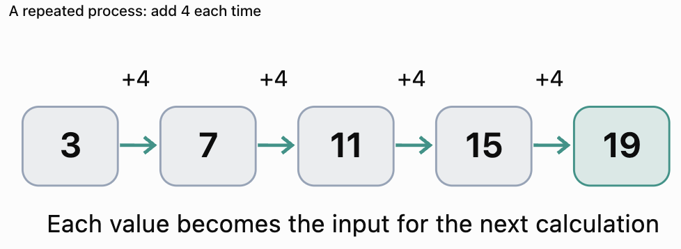
A recursive process follows a repeating cycle:
Previous value → Apply the rule → New value → Repeat
Generating Terms in Recursive Sequences
To generate a recursive sequence, begin with the initial condition and apply the recursive rule repeatedly.
Worked Example 1: An Additive Recursive Sequence
A sequence is defined by:
a₀ = 5
aₙ = aₙ₋₁ + 6
Find the first six terms, from a₀ to a₅.
Step 1: Start with the initial value.
a₀ = 5
Step 2: Apply the recursive rule.
a₁ = 5 + 6 = 11
a₂ = 11 + 6 = 17
a₃ = 17 + 6 = 23
a₄ = 23 + 6 = 29
a₅ = 29 + 6 = 35
Answer: 5, 11, 17, 23, 29, 35
This is an arithmetic sequence because the same amount is added each time.
Worked Example 2: A Multiplicative Recursive Sequence
A sequence is defined by:
a₀ = 2
aₙ = 3aₙ₋₁
Find the first five terms.
a₀ = 2
a₁ = 3 × 2 = 6
a₂ = 3 × 6 = 18
a₃ = 3 × 18 = 54
a₄ = 3 × 54 = 162
Answer: 2, 6, 18, 54, 162
This is a geometric sequence because each term is multiplied by 3.
Worked Example 3: A Two-Term Recursive Rule
Consider:
a₀ = 1
a₁ = 2
aₙ = aₙ₋₁ + aₙ₋₂, for n ≥ 2
Find a₂ through a₆.
a₂ = 2 + 1 = 3
a₃ = 3 + 2 = 5
a₄ = 5 + 3 = 8
a₅ = 8 + 5 = 13
a₆ = 13 + 8 = 21
Answer: 1, 2, 3, 5, 8, 13, 21
This is a Fibonacci-type sequence.
It differs from the previous examples because calculating each new term requires two earlier values.
Interactive Recursive Sequence Explorer
Explore how changing a recursive rule affects the values it generates.
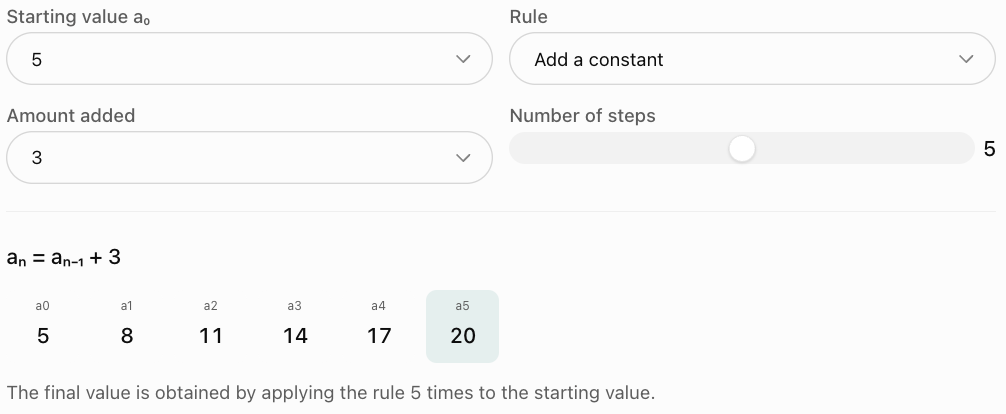
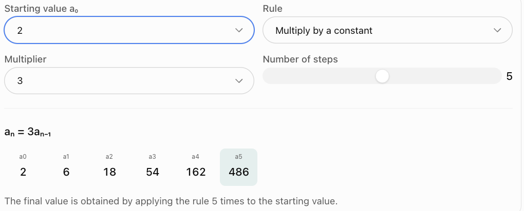
Notice that addition produces a constant difference, while multiplication produces a constant ratio.
Recursive Models of Arithmetic Sequences
An arithmetic sequence is a sequence in which the difference between consecutive terms is constant.
Its recursive rule is:
aₙ = aₙ₋₁ + d
where d is the common difference.
For example:
10, 15, 20, 25, 30, ...
Starting value:
a₀ = 10
Recursive rule:
aₙ = aₙ₋₁ + 5
Explicit form
The same sequence can be described by:
aₙ = a₀ + nd
For this example:
aₙ = 10 + 5n
To find a₂₀:
a₂₀ = 10 + 5(20)
a₂₀ = 110
The explicit formula allows us to calculate a term directly without finding all earlier terms.
Recursive Models of Geometric Sequences
A geometric sequence is formed by multiplying each term by a constant ratio.
The recursive rule is:
aₙ = raₙ₋₁
where r is the common ratio.
For example:
4, 8, 16, 32, 64, ...
Starting value:
a₀ = 4
Recursive rule:
aₙ = 2aₙ₋₁
Explicit form
The corresponding explicit formula is:
aₙ = a₀rⁿ
For this example:
aₙ = 4(2)ⁿ
Find a₇:
a₇ = 4(2)⁷
= 4 × 128
a₇ = 512
Both approaches describe the same sequence.
The recursive approach explains how each term develops from the previous term.
The explicit approach calculates any term directly.
Recursive Models of Population Growth
Population growth is one of the most important applications of recursive modelling.
Suppose a population increases by a fixed percentage during each time period.
The next population depends on the current population.
Let:
Pₙ = population after n time periods
P₀ = initial population
r = growth rate expressed as a decimal
The recursive model is:
Pₙ₊₁ = Pₙ(1 + r)
For example, a 12% increase gives a growth factor of:
1 + 0.12 = 1.12
Worked Example 4: Population Growth
A town has a population of 2,000 people.
The population grows by 12% each year.
Estimate the population after four years.
Step 1: Define the initial condition.
P₀ = 2,000
Step 2: Write the recursive rule.
Pₙ₊₁ = 1.12Pₙ
Step 3: Generate the values.
P₁ = 2,000 × 1.12 = 2,240
P₂ = 2,240 × 1.12 = 2,508.8
P₃ = 2,508.8 × 1.12 = 2,809.856
P₄ = 2,809.856 × 1.12 = 3,147.03872
Answer: Approximately 3,147 people after four years.
The intermediate values are mathematical expectations; actual populations contain whole people.
Explicit model
Because the population grows by a constant percentage, we can also use:
Pₙ = 2,000(1.12)ⁿ
At n = 4:
P₄ = 2,000(1.12)⁴
≈ 3,147
Both approaches produce the same result.
Graphing population growth
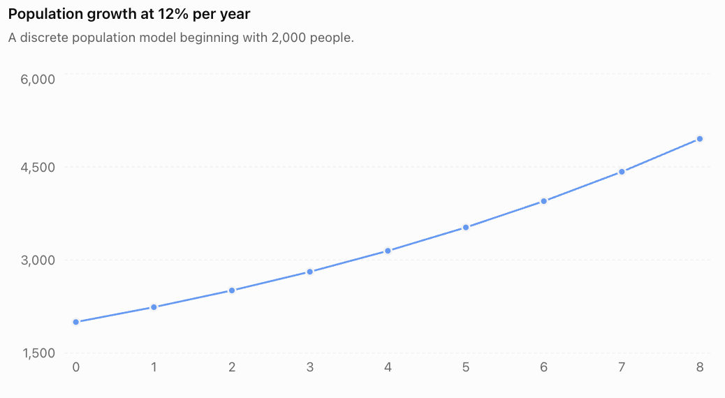
The graph curves upward because the same percentage is applied to an increasingly large population.
Interpreting the model
The model assumes:
-
The percentage growth rate remains constant.
-
The time periods are equal.
-
There are no unexpected major changes.
-
Resources and living conditions do not limit growth.
In reality, population growth may be affected by births, deaths, migration, disease, competition, and environmental conditions.
A recursive model is useful, but it is still a simplified representation of reality.
Recursive Models of Population Decline
Recursive models can also describe decreases.
Suppose a wildlife population decreases by 8% each year.
The population retains:
100% − 8% = 92%
of its previous value.
Therefore:
Pₙ₊₁ = 0.92Pₙ
Worked Example 5: Population Decline
A species has an initial population of 5,000.
The population decreases by 8% annually.
Estimate the population after three years.
P₀ = 5,000
P₁ = 5,000(0.92) = 4,600
P₂ = 4,600(0.92) = 4,232
P₃ = 4,232(0.92) = 3,893.44
Answer: Approximately 3,893 individuals.
The explicit model is:
Pₙ = 5,000(0.92)ⁿ
This is an example of exponential decay.
Population Models with a Fixed Change and Percentage Growth
Some populations change through more than one process.
For example, a town may grow naturally by a percentage each year while also receiving a fixed number of new residents.
Suppose:
-
Initial population = 1,000
-
Annual natural growth = 5%
-
Additional residents arriving each year = 100
The recursive rule is:
Pₙ₊₁ = 1.05Pₙ + 100
This combines multiplication and addition.
Worked Example 6: Growth and Migration
Find the population after three years.
P₀ = 1,000
P₁ = 1.05(1,000) + 100
= 1,150
P₂ = 1.05(1,150) + 100
= 1,307.5
P₃ = 1.05(1,307.5) + 100
= 1,472.875
Answer: Approximately 1,473 people.
This model is more complex than a simple geometric sequence.
The percentage growth is applied first, followed by the addition of 100 residents.
Changing the order of operations may change the model.
Recursive Models in Finance
Financial processes often involve repeated percentage changes, deposits, withdrawals, and payments.
Recursive models are particularly useful because each new balance depends on the previous balance.
Compound interest
Suppose a bank account earns interest at a fixed rate every year.
Let:
Aₙ = balance after n years
A₀ = initial balance
r = annual interest rate
The recursive rule is:
Aₙ₊₁ = Aₙ(1 + r)
This is the same mathematical structure as exponential population growth.
Worked Example 7: Compound Interest
An investment begins with $2,000 and earns 5% interest annually.
Find the balance after four years.
A₀ = 2,000
Aₙ₊₁ = 1.05Aₙ
A₁ = 2,000 × 1.05 = 2,100
A₂ = 2,100 × 1.05 = 2,205
A₃ = 2,205 × 1.05 = 2,315.25
A₄ = 2,315.25 × 1.05 = 2,431.0125
Answer: $2,431.01
The explicit formula is:
Aₙ = 2,000(1.05)ⁿ
Savings Models with Regular Deposits
Many people save money by making regular deposits into an account that earns interest.
Suppose a person:
-
Begins with $1,000.
-
Earns 4% interest annually.
-
Deposits $200 at the end of every year.
The recursive model is:
Aₙ₊₁ = 1.04Aₙ + 200
This means:
-
Calculate interest on the existing balance.
-
Add the annual deposit.
-
Use the result as the balance for the next year.
Worked Example 8: Savings with Deposits
Find the balance after three years.
A₀ = 1,000
Year 1:
A₁ = 1.04(1,000) + 200
= 1,240
Year 2:
A₂ = 1.04(1,240) + 200
= 1,489.60
Year 3:
A₃ = 1.04(1,489.60) + 200
= 1,749.184
Answer: $1,749.18
Interpreting the model
The account increases for two reasons:
-
Interest is earned on the previous balance.
-
A new deposit is added.
The balance does not form a simple geometric sequence because the fixed deposit changes the ratio between consecutive balances.
An explicit formula
For a constant interest rate and a fixed deposit made at the end of each period:
Aₙ = A₀(1 + r)ⁿ + d[(1 + r)ⁿ − 1]/r
where d is the deposit per period and r ≠ 0.
For the example:
A₃ = 1,000(1.04)³ + 200[(1.04)³ − 1]/0.04
= 1,124.864 + 624.32
= 1,749.184
This matches the recursive calculation.
If r = 0, the model simplifies to Aₙ = A₀ + nd.
Recursive Models for Loans
A loan balance changes through interest charges and repayments.
Suppose a borrower owes $10,000.
The loan charges 1% interest per month, and the borrower pays $500 at the end of each month.
Let Bₙ represent the outstanding balance after n payments.
The recursive rule is:
Bₙ₊₁ = 1.01Bₙ − 500
Worked Example 9: Loan Repayment
Find the outstanding balance after three payments.
Initial balance:
B₀ = 10,000
Month 1:
B₁ = 1.01(10,000) − 500
= 10,100 − 500
= 9,600
Month 2:
B₂ = 1.01(9,600) − 500
= 9,696 − 500
= 9,196
Month 3:
B₃ = 1.01(9,196) − 500
= 9,287.96 − 500
= 8,787.96
Answer: $8,787.96 remains after three payments.
Why the order matters
Interest is charged before the monthly payment is subtracted.
If the payment occurred at the beginning of the month, the recurrence would be different:
Bₙ₊₁ = 1.01(Bₙ − 500)
Real financial models must reflect the actual timing of deposits, payments, and interest.
Comparing Recursive and Explicit Models
Recursive and explicit models are two ways of describing mathematical sequences.
Recursive approach
A recursive rule calculates a term from one or more previous terms.
Example:
a₀ = 3
aₙ = 2aₙ₋₁
To find a₄:
a₁ = 6
a₂ = 12
a₃ = 24
a₄ = 48
Explicit approach
An explicit rule calculates a term directly from its position.
For the same sequence:
aₙ = 3(2)ⁿ
Therefore:
a₄ = 3(2)⁴
a₄ = 48
Comparison
|
Feature |
Recursive model |
Explicit model |
|---|---|---|
|
Uses previous values |
Yes |
Not necessarily |
|
Needs starting values |
Yes |
Constants determine the starting values |
|
Calculates distant terms directly |
Usually no |
Yes |
|
Describes step-by-step change |
Very clearly |
Less directly |
|
Useful for repeated processes |
Yes |
Yes |
|
Handles complex changing rules |
Often convenient |
May be difficult |
|
Easy to calculate using a spreadsheet |
Yes |
Yes |
When should each approach be used?
Use a recursive model when:
-
The process repeats in stages.
-
The next value depends on the previous value.
-
Deposits, withdrawals, or other changes occur regularly.
-
Different rules apply at different times.
-
A simple explicit formula is unavailable.
Use an explicit model when:
-
You need a distant term quickly.
-
The sequence follows a known formula.
-
You want to compare values at different times.
-
You want to solve for the time at which a threshold is reached.
Converting Recursive Models to Explicit Models
For arithmetic and geometric sequences, conversion is straightforward.
Arithmetic sequences
Recursive:
aₙ = aₙ₋₁ + d
Initial condition:
a₀ = A
Explicit:
aₙ = A + nd
Geometric sequences
Recursive:
aₙ = raₙ₋₁
Initial condition:
a₀ = A
Explicit:
aₙ = Arⁿ
Worked Example 10: Converting an Arithmetic Model
Given:
a₀ = 12
aₙ = aₙ₋₁ − 3
The common difference is −3.
Therefore:
aₙ = 12 − 3n
Find a₁₀:
a₁₀ = 12 − 3(10)
a₁₀ = −18
Worked Example 11: Converting a Geometric Model
Given:
a₀ = 80
aₙ = 0.75aₙ₋₁
The common ratio is 0.75.
Therefore:
aₙ = 80(0.75)ⁿ
Find a₄:
a₄ = 80(0.75)⁴
= 80(0.31640625)
a₄ = 25.3125
More Advanced Recursive Models
Not all recursive models are arithmetic or geometric.
Some contain multiple operations or depend on more than one previous term.
Linear first-order recurrence
A common model is:
aₙ₊₁ = raₙ + d
This combines multiplication by a constant with addition of another constant.
It can describe savings, loans, population changes, and other repeated processes.
When r ≠ 1, its explicit form is:
aₙ = rⁿa₀ + d(rⁿ − 1)/(r − 1)
When r = 1:
aₙ = a₀ + nd
Worked Example 12: A Combined Recursive Model
A sequence is defined by:
a₀ = 10
aₙ₊₁ = 2aₙ + 3
Find a₃.
a₁ = 2(10) + 3 = 23
a₂ = 2(23) + 3 = 49
a₃ = 2(49) + 3 = 101
Answer: 101
Using the explicit formula:
aₙ = 2ⁿ(10) + 3(2ⁿ − 1)
At n = 3:
a₃ = 8(10) + 3(7)
= 80 + 21
= 101
Both approaches agree.
Recursive Models and Long-Term Behaviour
Recursive models can help predict what happens after many repeated steps.
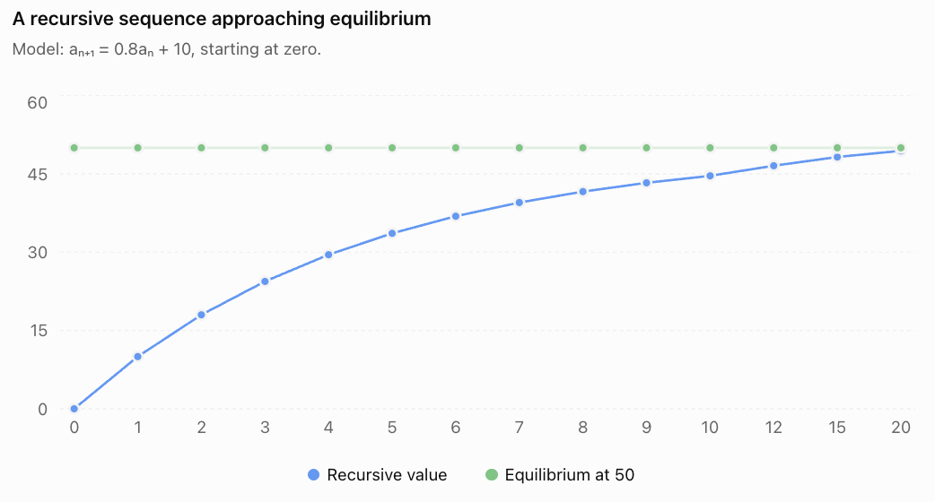
Consider:
aₙ₊₁ = 0.8aₙ + 10
with:
a₀ = 0
The first few terms are:
a₁ = 10
a₂ = 18
a₃ = 24.4
a₄ = 29.52
a₅ = 33.616
The values increase, but the increases become smaller.
The sequence approaches a limiting value.
Finding an equilibrium value
At equilibrium, the value no longer changes.
Let the equilibrium value be L.
Then:
L = 0.8L + 10
Subtract 0.8L:
0.2L = 10
Divide by 0.2:
L = 50
The sequence approaches 50.
Important observation
A fixed point is not always approached.
For a recurrence of the form aₙ₊₁ = raₙ + d, the fixed point is generally stable when:
|r| < 1
When |r| is greater than 1, values generally move away from the fixed point unless they begin exactly there.
This connects recursive sequences with the advanced mathematical study of dynamical systems.
Recursive Models and Technology
Recursive models are also important in computer science.
Computers can generate sequences by repeatedly applying a rule.
For example, a spreadsheet can calculate the next value from the previous row.
A simple algorithm for the model:
a₀ = 5
aₙ₊₁ = 1.2aₙ
could be written as:
value = 5
repeat 5 times:
value = value * 1.2
display value
The result is:
5(1.2)⁵ = 12.4416
This shows how recursion and iteration can be implemented computationally.
In mathematics, recursion describes a relationship using previous values.
In programming, iteration means repeatedly performing instructions. An iterative program can calculate a recursively defined sequence without a function calling itself.
Real-World Applications
Recursive models are used in many fields.
Population studies: Predicting populations through repeated births, deaths, and migration.
Finance: Calculating investment growth, savings balances, loan repayments, and depreciation.
Biology: Modelling population changes, reproduction, and repeated biological processes.
Environmental science: Modelling the amount of a pollutant remaining after repeated removal.
Medicine: Modelling drug concentrations when a fraction is eliminated between doses.
Computer science: Generating sequences and implementing repeated calculations.
Economics: Modelling changes in prices, production, and other quantities over time.
The same mathematical structure can describe very different situations.
For example:
Pₙ₊₁ = 1.05Pₙ
could represent a population growing by 5% per year.
Aₙ₊₁ = 1.05Aₙ
could represent an investment earning 5% interest per year.
The mathematics is identical, but the variables and interpretations differ.
Common Mistakes
Mistake 1: Forgetting the initial condition
A recursive rule usually requires one or more starting values.
Mistake 2: Confusing aₙ with aₙ₋₁
aₙ is the current term, while aₙ₋₁ is the preceding term.
Mistake 3: Applying a percentage incorrectly
A 6% increase means multiplying by 1.06, not by 0.06.
Mistake 4: Treating percentage growth as constant addition
A fixed percentage produces a changing absolute increase.
Mistake 5: Using the wrong number of time periods
If a₀ is the initial value, a₅ represents five completed steps.
Mistake 6: Changing the order of financial operations
Interest before a deposit is different from interest after a deposit.
Mistake 7: Assuming every recursive model is geometric
Models such as aₙ₊₁ = 1.05aₙ + 100 are not simple geometric sequences.
Mistake 8: Rounding intermediate values too early
Premature rounding can accumulate errors over many steps.
Mistake 9: Assuming recursive models always have simple explicit formulas
Some recursive models cannot be expressed using elementary explicit formulas.
Mistake 10: Extending a model without evaluating its assumptions
A constant population growth rate or interest rate may not remain realistic indefinitely.
Key Terms
-
Recursive Model: Mathematical model in which new values depend on earlier values.
-
Recursion: Process of defining or calculating values using previous values.
-
Recursive Rule: Equation that determines a term from earlier terms.
-
Initial Condition: Starting value needed to generate a recursive sequence.
-
Sequence: Ordered list of numbers following a rule.
-
Term: Individual value in a sequence.
-
Term Number: Position or index of a term.
-
Arithmetic Sequence: Sequence with a constant difference.
-
Geometric Sequence: Sequence with a constant ratio.
-
Common Difference: Constant amount added between arithmetic terms.
-
Common Ratio: Constant multiplier between geometric terms.
-
Explicit Formula: Formula that calculates a term directly from its index.
-
Growth Factor: Multiplier representing a percentage increase.
-
Decay Factor: Multiplier representing a percentage decrease.
-
Compound Interest: Interest calculated on the principal and accumulated interest.
-
Population Model: Mathematical representation of changes in population.
-
Fixed Point: Value that remains unchanged when a recursive rule is applied.
-
Equilibrium: State in which the model's value remains constant.
-
Long-Term Behaviour: Pattern shown by a model after many repeated steps.
-
Iteration: Repeated application of a calculation or procedure.
-
Dynamical System: Mathematical system describing how quantities change over time.
Key Takeaways
-
Recursive models describe processes in which each new value depends on earlier values.
-
A recursive model requires initial conditions.
-
Recursive rules can generate arithmetic, geometric, and more complex sequences.
-
Arithmetic recursive models add a constant amount each step.
-
Geometric recursive models multiply by a constant factor each step.
-
Population growth and decay can be described recursively.
-
Compound interest is a common example of a geometric recursive model.
-
Savings and loans often involve both percentage changes and fixed payments.
-
Recursive models are useful when changes occur in repeated stages.
-
Explicit models calculate terms directly from their position.
-
Recursive and explicit approaches can describe the same mathematical process.
-
Some recursive models approach equilibrium values.
-
Long-term predictions depend on the assumptions of the model.
-
Recursive thinking is important in mathematics, science, finance, and computing.
Check Your Understanding
Questions
Question 1: Understanding Recursion
Explain what a recursive model is and why an initial condition is important.
Question 2: Generating a Sequence
Given:
a₀ = 4
aₙ = aₙ₋₁ + 7
Find a₁ through a₅.
Question 3: Geometric Recursion
Given:
a₀ = 3
aₙ = 2aₙ₋₁
Find a₄.
Question 4: Identifying the Rule
Write a recursive rule for:
8, 13, 18, 23, 28, ...
Use a₀ = 8.
Question 5: Explicit Form
Convert:
a₀ = 6
aₙ = aₙ₋₁ + 4
into an explicit formula.
Question 6: Population Growth
A town has 1,500 residents and grows by 10% each year.
Write a recursive rule and estimate the population after three years.
Question 7: Population Decline
A population of 8,000 decreases by 5% annually.
Find the population after two years.
Question 8: Compound Interest
An investment of $3,000 earns 6% annual interest.
Calculate the balance after three years.
Question 9: Savings Model
An account begins with $500.
It earns 3% interest annually, and $100 is deposited at the end of each year.
Write the recursive model and calculate the balance after two years.
Question 10: Loan Model
A loan begins at $5,000.
Interest is charged at 2% per month, followed by a payment of $300.
Find the balance after two payments.
Question 11: Comparing Models
Explain one advantage of a recursive model and one advantage of an explicit model.
Question 12: Combined Recurrence
Given:
a₀ = 2
aₙ₊₁ = 3aₙ + 1
Find a₃.
Question 13: Equilibrium
A sequence follows:
aₙ₊₁ = 0.5aₙ + 20
Find its equilibrium value.
Question 14: Modelling a Real Situation
A wildlife population begins with 600 animals.
Each year the population grows by 8%, after which 20 animals are removed.
Write a recursive rule and calculate the population after two years.
Question 15: Integrated Challenge
A savings account begins with $2,000.
The account earns 5% annual interest, and $300 is deposited at the end of each year.
a) Write the recursive model.
b) Calculate the balance after three years.
c) Write an explicit formula.
d) Use the explicit formula to verify the result.
e) Explain one assumption of the model.
Fully Worked Answers
Answer 1: Understanding Recursion
A recursive model calculates new values using one or more previous values.
An initial condition provides the starting value.
Without the initial condition, the recursive rule may describe many different sequences.
Answer 2: Generating a Sequence
Given:
a₀ = 4
aₙ = aₙ₋₁ + 7
Calculate:
a₁ = 4 + 7 = 11
a₂ = 11 + 7 = 18
a₃ = 18 + 7 = 25
a₄ = 25 + 7 = 32
a₅ = 32 + 7 = 39
Answer: 11, 18, 25, 32, 39
Answer 3: Geometric Recursion
Given:
a₀ = 3
aₙ = 2aₙ₋₁
Calculate:
a₁ = 6
a₂ = 12
a₃ = 24
a₄ = 48
Answer: a₄ = 48
Answer 4: Identifying the Rule
Sequence:
8, 13, 18, 23, 28, ...
Each term increases by 5.
Initial condition:
a₀ = 8
Recursive rule:
aₙ = aₙ₋₁ + 5, for n ≥ 1
Answer 5: Explicit Form
Given:
a₀ = 6
Common difference:
d = 4
Explicit formula:
aₙ = a₀ + nd
aₙ = 6 + 4n
Answer 6: Population Growth
Initial population:
P₀ = 1,500
Growth rate:
10% = 0.10
Recursive rule:
Pₙ₊₁ = 1.10Pₙ
Calculate:
P₁ = 1,500(1.10) = 1,650
P₂ = 1,650(1.10) = 1,815
P₃ = 1,815(1.10) = 1,996.5
Answer: Approximately 1,997 residents after three years.
Answer 7: Population Decline
Initial population:
P₀ = 8,000
Decay factor:
1 − 0.05 = 0.95
Recursive model:
Pₙ₊₁ = 0.95Pₙ
Calculate:
P₁ = 8,000(0.95) = 7,600
P₂ = 7,600(0.95) = 7,220
Answer: 7,220 individuals
Answer 8: Compound Interest
Initial investment:
A₀ = 3,000
Growth factor:
1.06
Recursive model:
Aₙ₊₁ = 1.06Aₙ
Calculate:
A₁ = 3,180
A₂ = 3,370.80
A₃ = 3,573.048
Answer: $3,573.05
Answer 9: Savings Model
Initial balance:
A₀ = 500
Interest rate:
3%
Annual deposit:
$100
Recursive rule:
Aₙ₊₁ = 1.03Aₙ + 100
Calculate:
A₁ = 1.03(500) + 100
= 615
A₂ = 1.03(615) + 100
= 733.45
Answer: $733.45
Answer 10: Loan Model
Initial balance:
B₀ = 5,000
Monthly interest:
2%
Monthly payment:
$300
Recursive rule:
Bₙ₊₁ = 1.02Bₙ − 300
First payment:
B₁ = 1.02(5,000) − 300
= 4,800
Second payment:
B₂ = 1.02(4,800) − 300
= 4,896 − 300
Answer: $4,596
Answer 11: Comparing Models
A recursive model is useful because it describes how a quantity changes from one step to the next.
An explicit model is useful because it allows a distant term to be calculated directly.
For example, an explicit formula can calculate the balance after 20 years without calculating all 19 preceding balances.
Answer 12: Combined Recurrence
Given:
a₀ = 2
aₙ₊₁ = 3aₙ + 1
Calculate:
a₁ = 3(2) + 1 = 7
a₂ = 3(7) + 1 = 22
a₃ = 3(22) + 1 = 67
Answer: a₃ = 67
Answer 13: Equilibrium
Given:
aₙ₊₁ = 0.5aₙ + 20
At equilibrium:
L = 0.5L + 20
Subtract 0.5L:
0.5L = 20
Divide by 0.5:
L = 40
The equilibrium value is 40.
Because the multiplier is 0.5, values approach this equilibrium.
Answer 14: Modelling a Real Situation
Initial population:
P₀ = 600
Growth rate:
8%
Animals removed each year:
20
Recursive model:
Pₙ₊₁ = 1.08Pₙ − 20
Calculate:
P₁ = 1.08(600) − 20
= 648 − 20
= 628
P₂ = 1.08(628) − 20
= 678.24 − 20
= 658.24
Answer: Approximately 658 animals after two years.
The model treats population as a continuous numerical quantity for calculation purposes, so rounding is appropriate when interpreting the result.
Answer 15: Integrated Challenge
Part a: Write the recursive model
Initial balance:
A₀ = 2,000
Interest rate:
5%
Annual deposit:
$300
Recursive rule:
Aₙ₊₁ = 1.05Aₙ + 300
Part b: Calculate the balance after three years
Year 1:
A₁ = 1.05(2,000) + 300
= 2,400
Year 2:
A₂ = 1.05(2,400) + 300
= 2,820
Year 3:
A₃ = 1.05(2,820) + 300
= 3,261
Balance after three years: $3,261.00
Part c: Write the explicit formula
For regular end-of-year deposits:
Aₙ = A₀(1 + r)ⁿ + d[(1 + r)ⁿ − 1]/r
Substitute:
Aₙ = 2,000(1.05)ⁿ + 300[(1.05)ⁿ − 1]/0.05
Part d: Verify the result
For n = 3:
A₃ = 2,000(1.05)³ + 300[(1.05)³ − 1]/0.05
= 2,000(1.157625) + 300(0.157625)/0.05
= 2,315.25 + 945.75
A₃ = $3,261.00
The explicit formula confirms the recursive result.
Part e: Explain an assumption
The model assumes that the interest rate remains fixed at 5% annually and that the $300 deposit is made at the end of every year.
Changes in interest rates or deposit timing would require a different model.
Final Reflection
Recursive models provide a powerful way to describe repeated processes.
They help us understand how a quantity changes from one stage to the next, whether we are investigating population growth, financial investments, savings accounts, loan repayments, or mathematical sequences.
Recursive models also connect naturally with arithmetic and geometric sequences. In many cases, an explicit formula can be derived to calculate distant terms more efficiently.
More advanced recursive models can describe systems involving several simultaneous changes or values that approach equilibrium.
The most important lesson is that recursion allows us to model change as a repeated process. By understanding how one step leads to the next, we can predict future values, analyse patterns, and make informed decisions about real-world situations.