Graphing Geometric Sequences

Introduction

A geometric sequence is a sequence of numbers in which each term is obtained by multiplying the previous term by a constant value called the common ratio.

For example:

2, 4, 8, 16, 32, ...

Each term is multiplied by 2.

We can represent this sequence in several ways:

• As an ordered list of numbers.

• As a table of values.

• As an nth term formula.

• As points on a coordinate plane.

Graphing geometric sequences helps us understand how quantities change through repeated multiplication.

Unlike arithmetic sequences, which generally produce straight-line patterns, geometric sequences are associated with exponential relationships.

These relationships are important in mathematics, finance, biology, physics, and many other fields.

Reviewing Geometric Sequences

A geometric sequence has a constant ratio between consecutive terms.

Consider:

3, 9, 27, 81, 243, ...

Find the ratio between consecutive terms:

9/3 = 3

27/9 = 3

81/27 = 3

243/81 = 3

The common ratio is:

r = 3

The nth term formula for a geometric sequence is:

aₙ = a₁rⁿ⁻¹

where:

• aₙ represents the nth term.

• a₁ represents the first term.

• r represents the common ratio.

• n represents the term position.

Example

For:

3, 9, 27, 81, ...

a₁ = 3

r = 3

Therefore:

aₙ = 3 × 3ⁿ⁻¹

This formula allows us to calculate the value at any positive integer term position.

Creating a Table of Values

A table of values organises the term numbers and their corresponding values.

Consider:

2, 6, 18, 54, 162, ...

The common ratio is:

r = 3

Creating the Table

The first column shows the position of each term.

The second column shows its value.

Why Are Tables Useful?

Tables allow us to:

• Organise sequence information.

• Identify the common ratio.

• Generate ordered pairs for graphing.

• Compare values at different positions.

• Recognise patterns of growth or decay.

• Verify the nth term formula.

Extending the Table

Continue multiplying by 3:

The values increase rapidly because each term is three times the previous term.

Creating Tables from nth Term Formulas

Sometimes we are given a formula instead of a list of terms.

We can substitute different term numbers into the formula to create a table.

Worked Example

Create a table for the first five terms of:

aₙ = 4 × 2ⁿ⁻¹

Step 1: Substitute n = 1

a₁ = 4 × 2⁰

a₁ = 4

Step 2: Substitute n = 2

a₂ = 4 × 2¹

a₂ = 8

Step 3: Substitute n = 3

a₃ = 4 × 2²

a₃ = 16

Step 4: Substitute n = 4

a₄ = 4 × 2³

a₄ = 32

Step 5: Substitute n = 5

a₅ = 4 × 2⁴

a₅ = 64

Completed Table

The table is now ready to be used for graphing.

Turning a Table into Coordinates

Each row of a table can be written as an ordered pair.

An ordered pair has the form:

(x, y)

For geometric sequences:

• x represents the term number n.

• y represents the term value aₙ.

Consider:

4, 8, 16, 32, 64

The coordinates are:

(1, 4)

(2, 8)

(3, 16)

(4, 32)

(5, 64)

Important Observation

The first coordinate represents the term position.

The second coordinate represents the value at that position.

For example:

(3, 16)

means that the third term has a value of 16.

Graphing a Geometric Sequence

To graph a geometric sequence, plot its ordered pairs on a coordinate plane.

Worked Example

Graph:

2, 4, 8, 16, 32

Step 1: Create a Table

Step 2: Write the Coordinates

(1, 2)

(2, 4)

(3, 8)

(4, 16)

(5, 32)

Step 3: Label the Axes

Horizontal axis: term number n.

Vertical axis: term value aₙ.

Step 4: Plot the Points

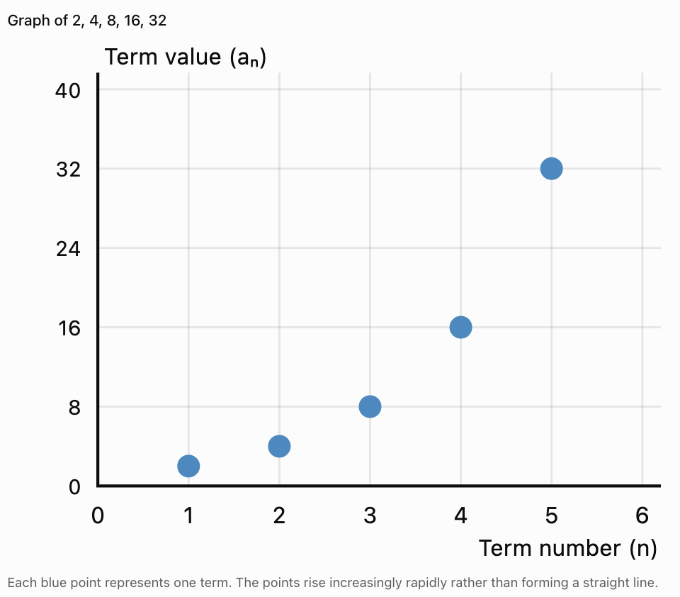
Step 5: Interpret the Graph

Notice that:

• The points rise from left to right.

• The vertical distance between consecutive points increases.

• Each term is twice the previous term.

• The points follow an exponential growth pattern.

The graph illustrates repeated multiplication rather than repeated addition.

Why Geometric Sequences Produce Exponential Patterns

Consider:

3, 6, 12, 24, 48, ...

The common ratio is 2.

Each time the term number increases by 1, the value doubles.

Comparing Changes

The differences increase.

However, the ratio remains constant.

What Does This Mean for the Graph?

The graph does not rise by the same vertical amount each time.

Instead, the vertical changes become larger as the terms increase.

This produces the increasingly steep pattern associated with exponential growth.

Important Distinction

Arithmetic sequences have constant first differences.

Geometric sequences have constant ratios.

For nonconstant positive geometric sequences, the points do not lie on a straight line.

Exponential Growth

A geometric sequence exhibits exponential growth when its positive terms increase through repeated multiplication by a factor greater than 1.

Example

5, 10, 20, 40, 80, 160, ...

First term:

a₁ = 5

Common ratio:

r = 2

nth term formula:

aₙ = 5 × 2ⁿ⁻¹

Table of Values

Interpreting the Graph

• The points rise increasingly rapidly.

• The values double with each new term.

• The differences between consecutive values become larger.

• The pattern represents exponential growth.

Common Ratios Greater Than 1

For a positive first term:

• r = 1.1 means a 10% increase per term.

• r = 1.5 means a 50% increase per term.

• r = 2 means the value doubles.

• r = 3 means the value triples.

Larger common ratios generally produce faster growth when the first term is the same.

Exponential Decay

A geometric sequence exhibits exponential decay when its positive terms decrease through repeated multiplication by a factor between 0 and 1.

Example

160, 80, 40, 20, 10, 5, ...

First term:

a₁ = 160

Common ratio:

r = 0.5

nth term formula:

aₙ = 160(0.5)ⁿ⁻¹

Table of Values

Graph Behaviour

• The points fall from left to right.

• The decreases become smaller in absolute size.

• The values approach zero.

• The sequence remains positive.

Important Observation

For a positive first term and 0 < r < 1, the terms approach zero as n increases.

However, they do not become exactly zero after any finite number of steps.

Comparing Different Rates of Exponential Decay

Consider two geometric sequences.

Sequence A:

100, 80, 64, 51.2, ...

Common ratio:

r = 0.8

Sequence B:

100, 50, 25, 12.5, ...

Common ratio:

r = 0.5

Comparison Table

Interpretation

Both sequences decrease.

However, Sequence B decreases faster because its common ratio is smaller.

Sequence A retains 80% of its previous value.

Sequence B retains only 50%.

Important Conclusion

For positive sequences with the same first term, a smaller positive common ratio between 0 and 1 produces faster decay.

Geometric Sequences with Negative Common Ratios

A geometric sequence may have a negative common ratio.

Consider:

2, −4, 8, −16, 32, ...

The common ratio is:

r = −2

Table of Values

Graph Behaviour

The plotted points alternate above and below the horizontal axis.

The absolute values increase because:

|r| = 2 > 1

Another Example

64, −32, 16, −8, 4, ...

Common ratio:

r = −0.5

The signs alternate, but the absolute values decrease.

Important Observation

A negative common ratio does not produce ordinary monotonic exponential growth or decay.

Instead, the sequence alternates in sign.

The absolute values may grow, decrease, or remain constant depending on |r|.

Geometric Sequences with a Common Ratio of 1

Consider:

7, 7, 7, 7, 7, ...

Common ratio:

r = 1

The nth term formula is:

aₙ = 7

Graph Behaviour

All points have the same vertical coordinate.

The graph forms a horizontal pattern.

This is a constant geometric sequence.

Special Case

A constant nonzero sequence is both:

• Arithmetic, with common difference d = 0.

• Geometric, with common ratio r = 1.

This is an important exception to the usual distinction between linear and exponential patterns.

Discrete and Continuous Graphs

Geometric sequences are normally represented by discrete points.

This is because term numbers are positive integers:

n = 1, 2, 3, 4, ...

Discrete Sequence

Consider:

aₙ = 2ⁿ

The first four terms are:

2, 4, 8, 16

The graph contains:

(1, 2), (2, 4), (3, 8), (4, 16)

There is no term at n = 2.5.

Continuous Exponential Function

Consider:

y = 2ˣ

This function is defined for all real x-values.

Its graph is a continuous exponential curve.

For example, at x = 2.5:

y = 2²⋅⁵ ≈ 5.657

This point belongs to the continuous exponential function but not to the discrete sequence indexed by positive integers.

Why Shouldn't We Connect the Points?

Connecting geometric sequence points with a solid curve can incorrectly suggest that fractional term positions are included.

A smooth curve may be drawn as a visual guide to the underlying exponential relationship, but the sequence itself consists of separate points.

Comparing Arithmetic and Geometric Graphs

Arithmetic and geometric sequences often behave very differently when graphed.

Consider two sequences.

Arithmetic:

2, 4, 6, 8, 10, 12, ...

Geometric:

2, 4, 8, 16, 32, 64, ...

Comparison Table

Comparing the Graphs

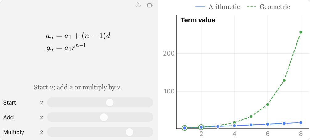
Arithmetic Graph

• The points lie on a straight line.

• The vertical change is constant.

• The common difference determines the slope.

• The pattern represents linear growth.

Geometric Graph

• The points follow an exponential pattern.

• The vertical change is not constant.

• The common ratio determines the multiplicative change.

• With a positive first term and r > 1, the values grow increasingly rapidly.

Important Conclusion

Linear growth adds a fixed amount.

Exponential growth multiplies by a fixed factor.

For positive starting values and a fixed growth ratio greater than 1, geometric growth eventually exceeds arithmetic growth with a fixed positive common difference.

Comparing Arithmetic and Geometric Growth Over Time

Suppose two savings plans begin with $100.

Plan A: Arithmetic Growth

The balance increases by $50 each year.

Sequence:

100, 150, 200, 250, 300, ...

Formula:

aₙ = 100 + 50(n − 1)

Plan B: Geometric Growth

The balance increases by 50% each year.

Sequence:

100, 150, 225, 337.50, 506.25, ...

Formula:

bₙ = 100(1.5)ⁿ⁻¹

Comparison

Interpretation

The arithmetic plan increases by the same dollar amount each year.

The geometric plan increases by the same percentage each year.

As the balance grows, the percentage increase produces larger dollar increases.

This causes the geometric sequence to grow more rapidly.

Interpreting Geometric Graphs in Real-World Situations

When interpreting a geometric sequence graph, consider:

• What does the horizontal axis represent?

• What does the vertical axis represent?

• What is the initial value?

• What is the common ratio?

• Does the quantity grow or decay?

• What does each plotted point represent?

• Are the values realistic?

• What assumptions does the model make?

These questions help connect mathematical patterns to meaningful real-world situations.

Real-World Application: Bacterial Growth

A bacterial population begins with 100 cells and doubles every hour under ideal conditions.

Create a Table

Formula

Let P(t) represent the expected population after t hours.

P(t) = 100 × 2ᵗ

Here the initial population is recorded at t = 0.

Interpreting the Graph

• Horizontal axis: time in hours.

• Vertical axis: bacterial population.

• Initial value: 100 cells.

• Common ratio: 2 per hour.

• Growth pattern: exponential.

Prediction

After 8 hours:

P(8) = 100 × 2⁸

P(8) = 100 × 256

P(8) = 25,600 cells

Model Limitation

Real bacterial populations do not grow exponentially forever.

Nutrient availability, space, waste accumulation, and other environmental factors eventually limit growth.

Real-World Application: Compound Interest

An investment begins with $2,000 and earns 5% interest annually, compounded once per year.

Each year, the balance is multiplied by:

1.05

Table of Values

Formula

A(t) = 2,000(1.05)ᵗ

Interpreting the Graph

• Horizontal axis: years elapsed.

• Vertical axis: investment value.

• Initial value: $2,000.

• Common ratio: 1.05.

• Percentage growth: 5% annually.

Prediction

After 10 years:

A(10) = 2,000(1.05)¹⁰

A(10) ≈ $3,257.79

Important Observation

The dollar amount of interest earned increases over time because interest is calculated on the growing balance.

Real-World Application: Radioactive Decay

A radioactive sample initially contains 800 mg of a radioactive isotope.

Its half-life is 5 years.

After every 5-year interval, the expected remaining mass is multiplied by 0.5.

Create a Table

Formula

Let M(t) represent the expected remaining mass after t years.

M(t) = 800(0.5)ᵗ⁄⁵

Interpreting the Graph

• Horizontal axis: time in years.

• Vertical axis: expected remaining mass.

• Initial value: 800 mg.

• Common ratio: 0.5 every five years.

• Pattern: exponential decay.

Prediction

After 30 years:

M(30) = 800(0.5)⁶

M(30) = 800/64

M(30) = 12.5 mg

Scientific Interpretation

Radioactive decay is random at the level of individual nuclei.

The exponential model describes the expected behaviour of a sufficiently large sample.

Real-World Application: Vehicle Depreciation

A vehicle is purchased for $30,000.

Its value decreases by 20% each year.

Each year, the vehicle retains:

100% − 20% = 80%

Therefore:

r = 0.8

Table of Values

Formula

V(t) = 30,000(0.8)ᵗ

Interpreting the Graph

• The graph decreases from left to right.

• The value decreases by 20% annually.

• The dollar amount lost becomes smaller each year.

• The value approaches zero in the mathematical model.

Model Limitation

Real vehicle values may not follow a constant depreciation rate.

Market conditions, vehicle condition, age, and demand affect actual prices.

Real-World Application: A Bouncing Ball

A ball is dropped from a height of 5 metres.

After each bounce, it rises to 70% of its previous maximum height.

Table of Values

Formula

Let H represent the maximum height after n bounces.

H = 5(0.7)ⁿ

Interpreting the Graph

• Horizontal axis: bounce number.

• Vertical axis: maximum height.

• Initial height: 5 m.

• Common ratio: 0.7.

• Pattern: exponential decay.

Important Observation

The heights decrease geometrically because each bounce reaches a fixed percentage of the previous height.

The graph is discrete because bounce numbers are whole numbers.

Finding the Common Ratio from a Graph

We can determine the common ratio by reading consecutive term values from a graph.

Worked Example

A graph contains the points:

(1, 4)

(2, 12)

(3, 36)

(4, 108)

Find the common ratio.

Step 1: Identify Consecutive Terms

a₁ = 4

a₂ = 12

Step 2: Divide

r = 12/4

r = 3

Step 3: Verify

36/12 = 3

108/36 = 3

The ratios are constant.

Therefore, the sequence is geometric.

nth Term Formula

aₙ = 4 × 3ⁿ⁻¹

Finding the Common Ratio from Nonconsecutive Points

Sometimes the graph provides two points that are not consecutive.

Worked Example

A geometric sequence graph contains:

(2, 6) and (5, 162)

Assume the common ratio is positive.

Step 1: Identify the Terms

a₂ = 6

a₅ = 162

Step 2: Compare the Terms

From term 2 to term 5, there are three multiplications by r.

Therefore:

162 = 6r³

Step 3: Solve

r³ = 162/6

r³ = 27

r = 3

Step 4: Find the First Term

a₂ = a₁r

6 = 3a₁

a₁ = 2

Final Formula

aₙ = 2 × 3ⁿ⁻¹

Verification

a₅ = 2 × 3⁴

a₅ = 2 × 81

a₅ = 162

The formula matches the graph.

Recognising Geometric Sequences from Graphs

A geometric sequence graph may show:

• Rapidly increasing positive values.

• Positive values decreasing toward zero.

• Alternating positive and negative values.

• A constant horizontal pattern.

However, appearance alone is not sufficient to prove that a sequence is geometric.

How to Verify

1. Read the term values from the graph.

2. Identify consecutive nonzero terms.

3. Divide each term by the previous term.

4. Check whether the ratios are constant.

Example

A graph contains:

(1, 3), (2, 9), (3, 27), (4, 81)

The ratios are:

9/3 = 3

27/9 = 3

81/27 = 3

Therefore, the sequence is geometric.

Non-Geometric Example

A graph contains:

(1, 2), (2, 5), (3, 10), (4, 17)

The ratios are:

5/2 = 2.5

10/5 = 2

17/10 = 1.7

The ratios are not constant.

Therefore, the sequence is not geometric.

Choosing an Appropriate Graph Scale

Geometric sequences can grow very quickly.

Consider:

2, 6, 18, 54, 162, 486, ...

The sixth term is much larger than the first.

If the vertical axis only extends to 100, the later terms will not fit.

Strategies

• Choose a vertical scale that includes all required values.

• Use intervals such as 10, 50, 100, or 500 where appropriate.

• Label axes clearly.

• Avoid changing the scale partway through an axis.

• Consider graphing fewer terms if the values become extremely large.

• Use logarithmic scales for advanced comparisons across very large ranges.

Important Observation

A poorly chosen scale can make an exponential pattern difficult to interpret.

Always inspect the range of values before drawing the graph.

Common Mistakes

Switching the axes

The term number belongs on the horizontal axis.

The term value belongs on the vertical axis.

Connecting sequence points with a continuous curve

A geometric sequence is normally discrete.

Confusing the common ratio with the common difference

Geometric sequences use repeated multiplication, not repeated addition.

Assuming all geometric graphs increase

Positive geometric sequences may increase, decrease, or remain constant.

Ignoring negative common ratios

Negative ratios produce alternating signs for nonzero terms.

Using an inappropriate graph scale

Exponential growth can produce very large values after only a few terms.

Confusing exponential decay with linear decrease

Exponential decay involves repeated multiplication by a factor between 0 and 1.

Assuming an exponential decay sequence reaches zero

Positive geometric sequences with 0 < r < 1 approach zero but do not become exactly zero after finitely many terms.

Using the wrong starting index

Some real-world models begin at time zero.

Standard sequence notation often begins at n = 1.

Interpreting a graph beyond realistic conditions

Real-world growth and decay models depend on assumptions that may eventually fail.

Key Terms

• Geometric Sequence: Sequence with a constant ratio between consecutive terms.

• Common Ratio: Fixed multiplier used to generate the next term.

• First Term: Value at position n = 1.

• nth Term: Value at position n.

• Table of Values: Organised list of input and output values.

• Ordered Pair: Pair of coordinates written as (x, y).

• Coordinate Plane: Plane formed by horizontal and vertical axes.

• Horizontal Axis: Axis representing the term number or independent variable.

• Vertical Axis: Axis representing the term value or dependent variable.

• Exponential Growth: Increase caused by repeated multiplication by a factor greater than 1.

• Exponential Decay: Decrease caused by repeated multiplication by a factor between 0 and 1.

• Discrete Graph: Graph containing separate points at specified input values.

• Continuous Graph: Graph defined across an interval of real values.

• Arithmetic Sequence: Sequence with a constant difference between consecutive terms.

• Linear Relationship: Relationship with a constant rate of additive change.

• Exponential Relationship: Relationship involving repeated multiplication.

• Initial Value: Starting value of a model.

• Growth Factor: Multiplier greater than 1 representing repeated growth.

• Decay Factor: Multiplier between 0 and 1 representing repeated decay.

• Depreciation: Decrease in value over time.

• Compound Interest: Interest calculated on both the original investment and previously earned interest.

• Half-Life: Time required for half of a radioactive sample's undecayed nuclei to decay on average.

• Mathematical Model: Mathematical representation of a real-world situation.

• Prediction: Calculation of an unknown value using a mathematical relationship.

• Graph Scale: Numerical intervals used along graph axes.

Key Takeaways

• Geometric sequences can be represented using tables, formulas, and graphs.

• The term number is plotted on the horizontal axis.

• The term value is plotted on the vertical axis.

• Geometric sequences have a constant ratio between consecutive terms.

• The nth term formula is aₙ = a₁rⁿ⁻¹.

• Geometric sequence graphs generally follow exponential patterns.

• Positive common ratios greater than 1 produce exponential growth for positive first terms.

• Positive common ratios between 0 and 1 produce exponential decay for positive first terms.

• Negative common ratios produce alternating signs.

• Arithmetic sequence graphs form linear patterns.

• Geometric sequence graphs are normally discrete.

• Geometric growth can eventually exceed linear growth by a large amount.

• The common ratio can be calculated from graph coordinates.

• Tables help organise values before graphing.

• Real-world geometric graphs can model populations, investments, depreciation, and radioactive decay.

• Mathematical models must be interpreted within realistic conditions.

Check Your Understanding

Tables of Values

1. Create a table for the first five terms of 2, 4, 8, 16, ...

2. Create a table for the first five terms of aₙ = 3 × 2ⁿ⁻¹.

3. Create a table for the first five terms of aₙ = 80(0.5)ⁿ⁻¹.

4. Write the ordered pairs for 5, 15, 45, 135, ...

Graphing

5. Which variable belongs on the horizontal axis?

6. Which variable belongs on the vertical axis?

7. Why are geometric sequence graphs normally discrete?

8. Describe the graph of 4, 8, 16, 32, ...

Growth and Decay

9. Does a common ratio of 3 represent growth or decay for a positive first term?

10. Does a common ratio of 0.25 represent growth or decay for a positive first term?

11. Describe the graph of 100, 50, 25, 12.5, ...

12. Describe the graph of 3, −6, 12, −24, ...

Comparing Sequences

13. Explain how arithmetic and geometric graphs differ.

14. Compare the sequences 2, 4, 6, 8, ... and 2, 4, 8, 16, ...

15. Which grows faster for large n: aₙ = 3n or bₙ = 3ⁿ?

16. Explain why a geometric sequence with r = 1 produces a horizontal graph.

Applications

17. A bacterial population begins with 50 cells and doubles every hour. Find the expected population after five hours.

18. An investment of $1,000 grows by 10% annually. Write its value after three years.

19. A vehicle worth $20,000 loses 20% of its value each year. Find its value after four years.

20. A radioactive sample begins with 640 mg and halves every five years. Find the expected remaining mass after 15 years.

Answer Key

Extended Challenge

Creating Tables and Graphs

1. Create a table and graph for the first six terms of aₙ = 4 × 2ⁿ⁻¹.

2. Create a table and graph for the first six terms of aₙ = 128(0.5)ⁿ⁻¹.

3. Graph the first six terms of 3, −6, 12, −24, ...

4. Graph the first six terms of 5, 5, 5, 5, ...

5. Compare the graphs of aₙ = 2 × 3ⁿ⁻¹ and bₙ = 2 × 2ⁿ⁻¹.

Finding Formulas from Graph Data

6. Find the nth term formula for points (1, 3), (2, 9), (3, 27).

7. Find the nth term formula for points (1, 100), (2, 50), (3, 25).

8. A geometric sequence graph contains (2, 12) and (5, 324). Find the common ratio and nth term formula.

9. A geometric sequence has a first term of 5 and a common ratio of −2. Write its formula and graph the first five terms.

10. A geometric sequence has a first term of 200 and a common ratio of 0.8. Graph the first six terms.

Comparing Linear and Exponential Growth

11. Compare the first eight terms of aₙ = 5n and bₙ = 5 × 2ⁿ⁻¹.

12. Determine the first term position where bₙ = 3ⁿ exceeds aₙ = 10n.

13. Explain why exponential growth can eventually exceed linear growth.

14. Explain why exponential decay differs from a constant decrease.

15. Describe how changing the common ratio affects the shape of a geometric sequence graph.

Real-World Applications

16. A bacterial population begins with 200 cells and triples every hour. Graph the expected population over the first five hours.

17. An investment begins at $5,000 and grows by 6% annually. Graph its value over the first six years.

18. A radioactive sample begins with 1,024 mg and halves every four years. Graph the expected remaining mass over 20 years at four-year intervals.

19. A vehicle worth $40,000 loses 15% of its value annually. Graph its value over the first five years.

20. A ball rebounds to 75% of its previous maximum height. If dropped from 8 metres, graph the maximum heights after the first five bounces, including the initial height.

Final Challenge: Comparing Growth and Decay

Two geometric sequences are defined by:

Sequence A: aₙ = 5 × 2ⁿ⁻¹

Sequence B: bₙ = 160(0.5)ⁿ⁻¹

Complete the investigation.

1. Identify the first term of Sequence A.

2. Identify the first term of Sequence B.

3. Determine the common ratio of each sequence.

4. Create a table for the first eight terms of both sequences.

5. Write the coordinates for the first five terms of each sequence.

6. Plot both sequences on the same coordinate plane.

7. Describe the graphical pattern of Sequence A.

8. Describe the graphical pattern of Sequence B.

9. Explain why Sequence A represents exponential growth.

10. Explain why Sequence B represents exponential decay.

11. Determine the third term of each sequence.

12. Determine the fifth term of each sequence.

13. Calculate the tenth term of each sequence.

14. Explain how the common ratios affect the graph shapes.

15. Compare the vertical changes between consecutive points.

16. Explain why the graphs are discrete.

17. Determine whether the sequences ever have equal values at the same positive integer term position.

18. Describe a real-world situation that could be modelled by Sequence A.

19. Describe a real-world situation that could be modelled by Sequence B.

20. Explain why understanding exponential growth and decay is important in mathematics and science.

Further Investigation: Design Your Own Geometric Graphs

Create three geometric sequences:

• Sequence A: Exponential growth with a positive common ratio greater than 1.

• Sequence B: Exponential decay with a positive common ratio between 0 and 1.

• Sequence C: Alternating signs with a negative common ratio.

For each sequence:

1. Identify the first term.

2. Identify the common ratio.

3. Write the nth term formula.

4. Generate the first eight terms.

5. Create a table of values.

6. Write the ordered pairs.

7. Plot the sequence on a coordinate plane.

8. Describe the graphical pattern.

9. Predict the tenth term.

10. Explain how the graph differs from an arithmetic sequence.

11. Identify a possible real-world application.

12. Explain any limitations of the model.