Introduction to Linear Relationships

Introduction

Mathematics helps us recognise patterns, describe relationships, and predict what will happen when quantities change.

Many everyday situations involve two quantities that are connected. For example:

• The number of hours worked and the money earned.

• The number of notebooks purchased and their total cost.

• The distance travelled and the time spent moving.

• The amount of water in a tank as it fills.

• The total cost of a taxi ride as the distance increases.

When one quantity changes at a constant rate compared with another, the relationship is called a linear relationship.

Linear relationships can be represented using tables, equations, graphs, and written descriptions.

Learning to recognise linear patterns allows us to create mathematical rules and use them to make predictions.

What Is a Linear Relationship?

A linear relationship is a relationship between two variables that has a constant rate of change.

A linear relationship can be represented by an equation of the form:

y = mx + b

where:

• x = independent variable or input

• y = dependent variable or output

• m = constant rate of change, or slope

• b = initial value, or y-intercept

Example

A taxi charges a $4 starting fee plus $2 for every kilometre travelled.

The total cost can be represented by:

C = 2d + 4

where:

• C = total cost in dollars

• d = distance travelled in kilometres

• 2 = cost per kilometre

• 4 = starting fee

This is a linear relationship because the total cost increases by $2 for every additional kilometre.

Important Observation

A linear relationship does not have to begin at zero.

The starting value may be positive, negative, or zero.

Understanding Input and Output

A mathematical relationship often connects an input to an output.

The input is the value we choose or measure.

The output is the value calculated from the input.

Example

Consider the rule:

y = 3x + 2

If x = 1:

y = 3(1) + 2 = 5

If x = 2:

y = 3(2) + 2 = 8

If x = 3:

y = 3(3) + 2 = 11

Input-Output Table

Observations

• Every increase of 1 in x produces an increase of 3 in y.

• The output starts at 2 when x = 0.

• The relationship has a constant rate of change.

Therefore, the relationship is linear.

Recognising Patterns in Input-Output Tables

An input-output table organises corresponding values of two variables.

Example

Examine the changes in the output values.

6 → 10 → 14 → 18 → 22

Each output increases by 4.

Since the inputs increase by 1 each time, the rate of change is:

m = 4

Finding the Rule

Start with:

y = 4x + b

Use the point (1, 6):

6 = 4(1) + b

6 = 4 + b

b = 2

Therefore:

y = 4x + 2

Checking

When x = 5:

y = 4(5) + 2

y = 22

The equation matches the table.

Constant Rate of Change

The rate of change describes how much the output changes compared with the input.

For a linear relationship:

Rate of change = Change in output ÷ Change in input

Using symbols:

m = Δy/Δx

where:

• Δy = change in y

• Δx = change in x

Worked Example

Consider:

Step 1: Calculate the Change in x

4 − 2 = 2

Step 2: Calculate the Change in y

13 − 7 = 6

Step 3: Calculate the Rate

m = 6/2

m = 3

Check Another Interval

(19 − 13)/(6 − 4) = 6/2 = 3

The rate of change remains constant.

Therefore, the relationship is linear.

Important Observation

When input values increase by more than 1, the output differences must be divided by the corresponding input differences.

Recognising Linear and Nonlinear Patterns

Not all numerical patterns are linear.

Linear Pattern

The output increases by 3 for every increase of 1 in x.

The rate of change is constant.

Nonlinear Pattern

The output differences are:

3, 5, 7

The differences are not constant.

Therefore, the relationship is nonlinear.

The equation is:

y = x²

Important Observation

A linear pattern has a constant rate of change, not simply an increasing or decreasing sequence of outputs.

Finding Algebraic Rules from Tables

An algebraic rule is an equation describing how the output depends on the input.

Worked Example

Determine the rule for:

Step 1: Identify the Rate of Change

The output increases by 3 whenever x increases by 1.

Therefore:

m = 3

Step 2: Identify the Initial Value

When x = 0:

y = 5

Therefore:

b = 5

Step 3: Write the Equation

y = 3x + 5

Step 4: Verify

When x = 4:

y = 3(4) + 5

y = 17

The rule matches the table.

Finding a Rule When the Table Does Not Include Zero

Sometimes a table does not contain x = 0.

In this situation, use a known input-output pair to find the initial value.

Worked Example

Step 1: Calculate the Rate of Change

m = (19 − 11)/(4 − 2)

m = 8/2

m = 4

Step 2: Write the General Equation

y = 4x + b

Step 3: Substitute a Known Point

Use (2, 11):

11 = 4(2) + b

11 = 8 + b

b = 3

Final Equation

y = 4x + 3

Verification

When x = 8:

y = 4(8) + 3

y = 35

The equation is correct.

Positive, Negative, and Zero Rates of Change

Linear relationships can increase, decrease, or remain constant.

Positive Rate of Change

y = 2x + 1

As x increases, y increases.

The graph rises from left to right.

Negative Rate of Change

y = −3x + 10

As x increases, y decreases.

The graph falls from left to right.

Zero Rate of Change

y = 5

The output remains 5 regardless of the input.

The graph is horizontal.

Comparison

Exploring Linear Relationships Graphically

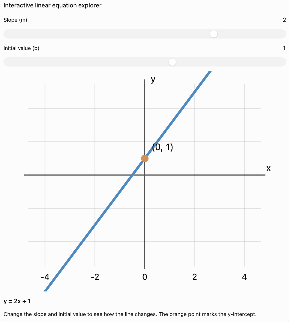
A linear equation produces a straight-line graph.

The slope determines the direction and steepness of the line.

The y-intercept determines where the line crosses the y-axis.

Questions to Consider

• What happens when the slope increases?

• What happens when the slope becomes negative?

• What happens when the slope is zero?

• What happens when the initial value changes?

• Why does the graph remain a straight line?

Linear Relationships and Direct Variation

Direct variation is a special type of linear relationship.

Direct Variation

y = kx

The initial value is zero.

The graph passes through the origin.

General Linear Relationship

y = mx + b

The initial value may be nonzero.

Example

A worker earns $15 per hour without any starting bonus.

E = 15h

This is direct variation.

Another worker earns $15 per hour plus a $20 starting bonus.

E = 15h + 20

This is linear but not directly proportional.

Important Observation

All direct variation relationships are linear, but not all linear relationships are direct variation.

Predicting Values Using Linear Rules

Once a linear equation is known, it can be used to predict outputs for different inputs.

Worked Example

A machine produces 12 items per minute and has already produced 30 items.

The total number of items is:

P = 12t + 30

where t is the number of additional minutes.

Predict Production After 8 Minutes

P = 12(8) + 30

P = 96 + 30

P = 126 items

Determine the Time Needed to Reach 210 Items

210 = 12t + 30

180 = 12t

t = 15 minutes

Important Observation

Linear equations can be used to calculate either an output or an input.

Linear Relationships in Shopping

Many shopping situations can be represented using linear equations.

Worked Example

A store charges $6 for delivery plus $4 per item.

Let:

n = number of items

C = total cost in dollars

Equation

C = 4n + 6

Create a Table

Interpretation

• Rate of change = $4 per item.

• Initial value = $6 delivery charge.

Prediction

For 10 items:

C = 4(10) + 6

C = $46

Linear Relationships in Transportation

Transportation costs often contain both a fixed fee and a variable fee.

Worked Example

A taxi charges:

• $5 starting fee

• $2.50 per kilometre

Equation

C = 2.5d + 5

where:

• C = cost in dollars

• d = distance in kilometres

Calculate the Cost of a 12 km Journey

C = 2.5(12) + 5

C = 30 + 5

C = $35

Find the Distance for a $55 Fare

55 = 2.5d + 5

50 = 2.5d

d = 20 km

Interpretation

The slope represents the cost per kilometre.

The y-intercept represents the starting fee.

Linear Relationships in Science

Linear relationships appear in many scientific situations.

Temperature Conversion

The relationship between Celsius and Fahrenheit temperatures is:

F = 1.8C + 32

where:

• F = temperature in degrees Fahrenheit

• C = temperature in degrees Celsius

Worked Example

Convert 25°C to Fahrenheit.

F = 1.8(25) + 32

F = 45 + 32

F = 77°F

Interpretation

The slope is 1.8.

The initial value is 32, meaning 0°C corresponds to 32°F.

Important Observation

Temperature conversion is linear but not directly proportional because the equation contains a nonzero initial value.

Linear Relationships in Water Usage

Suppose a water tank initially contains 150 litres.

Water flows into the tank at a constant rate of 20 litres per minute.

The amount of water after t minutes is:

V = 20t + 150

Worked Example

Find the volume after 6 minutes.

V = 20(6) + 150

V = 120 + 150

V = 270 L

Finding the Time

How long will it take to reach 350 litres?

350 = 20t + 150

200 = 20t

t = 10 minutes

Important Observation

This model is valid while the water flows at a constant rate and the tank has sufficient capacity.

Using Two Points to Determine a Linear Rule

Sometimes we know only two points on a line.

We can use these points to calculate the slope.

Formula

m = (y₂ − y₁)/(x₂ − x₁)

Worked Example

A linear relationship passes through:

(2, 7) and (6, 19)

Step 1: Calculate the Slope

m = (19 − 7)/(6 − 2)

m = 12/4

m = 3

Step 2: Write the General Equation

y = 3x + b

Step 3: Substitute a Known Point

Use (2, 7):

7 = 3(2) + b

7 = 6 + b

b = 1

Final Equation

y = 3x + 1

Verification

When x = 6:

y = 3(6) + 1

y = 19

The equation matches the second point.

Comparing Linear Relationships

Two linear relationships can be compared by examining their slopes and initial values.

Example

Company A charges:

C = 5x + 10

Company B charges:

C = 7x + 2

where x is the number of items purchased.

Comparing Initial Values

Company A starts at $10.

Company B starts at $2.

Comparing Rates

Company A increases by $5 per item.

Company B increases by $7 per item.

Finding Equal Costs

5x + 10 = 7x + 2

8 = 2x

x = 4

At x = 4:

Company A:

5(4) + 10 = $30

Company B:

7(4) + 2 = $30

Interpretation

Both companies charge $30 for 4 items.

For fewer than 4 items, Company B is cheaper.

For more than 4 items, Company A is cheaper.

Checking Linear Rules

After finding an algebraic rule, it should be verified.

Example

Suppose a table suggests:

y = 4x − 3

Check the point (5, 17).

Substitute:

y = 4(5) − 3

y = 20 − 3

y = 17

The equation matches the point.

Additional Checks

• Does the equation match every point in the table?

• Is the rate of change constant?

• Does the initial value make sense?

• Are the units appropriate?

• Are predictions reasonable within the situation?

Important Observation

Checking more than one point reduces the chance of accepting an incorrect rule.

A General Method for Finding Linear Rules

Common Mistakes

Assuming every pattern is linear

Check that the rate of change remains constant.

Looking only at output differences

If the input intervals differ, calculate Δy/Δx.

Confusing slope with initial value

The slope describes the rate of change; the initial value describes the output when x = 0.

Assuming all linear relationships are proportional

A proportional relationship must pass through the origin.

Making sign errors

A decreasing relationship has a negative slope.

Forgetting to calculate b

When the table does not include x = 0, use a known point to determine the initial value.

Using the wrong variables

Define inputs and outputs clearly.

Ignoring units

Rates may be measured in dollars per item, litres per minute, or kilometres per hour.

Making unrealistic predictions

Linear models may only apply over a particular range.

Failing to verify

Substitute known values into the equation to check the rule.

Key Terms

• Linear Relationship: Relationship with a constant rate of change.

• Input: Independent variable used in a mathematical rule.

• Output: Dependent variable produced by a mathematical rule.

• Input-Output Table: Table displaying corresponding values of two variables.

• Independent Variable: Variable that is chosen or controlled.

• Dependent Variable: Variable whose value depends on another.

• Algebraic Rule: Equation describing a relationship between variables.

• Rate of Change: Change in output divided by change in input.

• Slope: Constant rate of change of a straight line.

• Initial Value: Output when the input equals zero.

• y-Intercept: Point where a graph crosses the y-axis.

• Slope-Intercept Form: y = mx + b.

• Positive Slope: Rate of change greater than zero.

• Negative Slope: Rate of change less than zero.

• Zero Slope: Rate of change equal to zero.

• Direct Variation: Linear relationship represented by y = kx.

• Constant of Proportionality: Fixed multiplier in a proportional relationship.

• Linear Equation: Equation whose graph is a straight line.

• Nonlinear Relationship: Relationship without a constant rate of change.

• Ordered Pair: Pair of coordinates written as (x, y).

• Prediction: Calculated estimate using a mathematical rule.

• Substitution: Replacing a variable with a known value.

• Verification: Checking whether an equation matches the given data.

Key Takeaways

• Linear relationships have a constant rate of change.

• Input-output tables help identify numerical patterns.

• A linear equation can be written as y = mx + b.

• The slope m represents the rate of change.

• The initial value b represents the output when x = 0.

• A positive slope produces an increasing relationship.

• A negative slope produces a decreasing relationship.

• A zero slope produces a constant output.

• Linear graphs are straight lines.

• Direct variation is a special type of linear relationship.

• A linear relationship does not have to pass through the origin.

• The rate of change can be calculated using Δy/Δx.

• Two points with different x-values determine a unique linear rule.

• Linear equations can be used to predict unknown values.

• Mathematical rules should be verified using known data.

• Real-world predictions must be interpreted using appropriate units and assumptions.

Check Your Understanding

Recognising Patterns

1. What is a linear relationship?

2. What does the slope represent?

3. What does the y-intercept represent?

4. Is y = 5x + 3 linear?

5. Is y = x² + 2 linear?

Finding Rules

6. Find the rule for x = 0, 1, 2, 3 and y = 4, 7, 10, 13.

7. Find the rule for x = 0, 1, 2, 3 and y = 10, 8, 6, 4.

8. Find the slope between (2, 5) and (4, 11).

9. Find the equation of a line with slope 4 and y-intercept −2.

10. Find the equation passing through (0, 6) and (3, 15).

Predicting Values

11. If y = 3x + 5, find y when x = 8.

12. If y = −2x + 12, find y when x = 4.

13. If y = 5x − 3, find x when y = 22.

14. If C = 4n + 6, find the cost when n = 10.

15. If V = 15t + 100, find the volume when t = 8.

Understanding Linear Relationships

16. Explain why y = 4x is directly proportional.

17. Explain why y = 4x + 5 is not directly proportional.

18. What does a negative slope indicate?

19. How can you determine whether a table represents a linear relationship?

20. Why is it important to verify a linear equation?

Answer Key

Extended Challenge

1. Find the linear rule for the points (2, 9), (4, 15), (6, 21), and (8, 27).

2. Determine whether the points (1, 4), (2, 7), (3, 10), and (4, 13) form a linear relationship.

3. Find the equation of the line through (3, 11) and (7, 27).

4. A taxi charges $6 initially and $2.50 per kilometre. Write an equation and find the cost of a 14 km trip.

5. A tank begins with 250 litres and loses 12 litres per minute. Write an equation for its volume and determine when it becomes empty, assuming the rate stays constant.

6. Company A charges $8 per item plus $15 delivery. Company B charges $10 per item plus $5 delivery. Determine when the costs are equal.

7. A worker earns $18 per hour plus a $50 bonus. Write an equation and determine earnings after 12 hours.

8. Determine the rate of change for the points (2, 20) and (8, 8).

9. Find the equation of a line with slope −3 passing through (4, 7).

10. Explain how you would distinguish a linear relationship from a quadratic relationship using an input-output table.

Final Investigation: Planning a School Event

A school is organising an event and needs to compare costs from two suppliers.

Supplier A

Supplier A charges:

• $5 per student

• $40 fixed booking fee

Supplier B

Supplier B charges:

• $7 per student

• $10 fixed booking fee

Part A: Constructing Linear Models

1. Define the independent variable.

2. Define the dependent variable.

3. Write an equation for Supplier A.

4. Write an equation for Supplier B.

5. Identify the slope and initial value of each equation.

Part B: Creating Tables

6. Calculate the cost for 0 students.

7. Calculate the cost for 10 students.

8. Calculate the cost for 20 students.

9. Calculate the cost for 30 students.

10. Organise the results in an input-output table.

Part C: Comparing Relationships

11. Graph both equations on the same coordinate plane.

12. Determine which supplier has the greater rate of change.

13. Determine which supplier has the lower starting fee.

14. Calculate the number of students at which both suppliers charge the same amount.

15. Determine the common cost at that number of students.

Part D: Predictions and Interpretation

16. Calculate the cost from each supplier for 50 students.

17. Determine which supplier is cheaper for 50 students.

18. Explain which supplier is better for smaller groups.

19. Explain which supplier is better for larger groups.

20. Write a conclusion explaining how linear equations can help organisers make informed decisions.

Investigation Check

Supplier A

C = 5n + 40

Supplier B

C = 7n + 10

Equal Costs

5n + 40 = 7n + 10

30 = 2n

n = 15 students

At 15 students:

C = 5(15) + 40

C = $115

For 50 Students

Supplier A:

5(50) + 40 = $290

Supplier B:

7(50) + 10 = $360

Supplier A is cheaper by $70.

Conclusion

Supplier B is cheaper for fewer than 15 students, both cost the same for 15 students, and Supplier A is cheaper for more than 15 students.