Motion Graphs
5. Graphical Problem Solving
Learning outcomes
- I can use graphs to solve motion-related problems.
- I can combine information from multiple graph types.
- I can extract quantitative information from motion graphs.
- I can explain my reasoning using graphical evidence.
- I can apply graph analysis to real-world motion situations.
Why use graphs to solve motion problems?
Motion graphs show how quantities such as position, velocity and acceleration change over time. They can reveal information that may be difficult to recognize from an equation or written description.
Graphs can help us determine:
- Where an object is located.
- How fast it is moving.
- Which direction it is moving.
- Whether it is speeding up or slowing down.
- How far it travels.
- When its motion changes.
- Whether two objects meet.
To solve a graphical problem successfully, begin by identifying the quantities and units shown on the axes.
The main types of motion graphs
Position–time graphs
A position–time graph shows an object’s position relative to a chosen origin.
The vertical coordinate gives the object’s position.
The gradient gives velocity:
Velocity = change in position ÷ change in time
v = Δx / Δt
A positive gradient represents motion in the positive direction. A negative gradient represents motion in the negative direction.
Distance–time graphs
A distance–time graph usually shows the total distance travelled.
Its gradient gives speed:
Speed = change in distance ÷ change in time
The total distance normally cannot decrease, so a cumulative distance–time graph should not slope downwards.
Velocity–time graphs
A velocity–time graph shows the object’s velocity at each moment.
Its gradient gives acceleration:
Acceleration = change in velocity ÷ change in time
a = Δv / Δt
The signed area between the graph and the time axis gives displacement.
Speed–time graphs
A speed–time graph shows how quickly an object moves without representing direction.
Its gradient gives the rate of change of speed, and the area under the graph gives distance travelled.
Acceleration–time graphs
An acceleration–time graph shows how acceleration changes.
The signed area under the graph gives the change in velocity:
Change in velocity = area under an acceleration–time graph
This relationship allows us to move from an acceleration graph to a velocity graph.
Connecting the graph types
The same motion can be represented using several different graphs.
| Starting graph | Use the gradient to find | Use the signed area to find |
|---|---|---|
| Position–time | Velocity | — |
| Velocity–time | Acceleration | Displacement |
| Acceleration–time | — | Change in velocity |
These relationships form a chain:
Position → gradient → velocity → gradient → acceleration
Working in the opposite direction involves accumulation:
Acceleration → signed area → change in velocity → signed area → displacement
An area alone gives a change. An initial value is needed to find the final quantity.
For example:
Final velocity = initial velocity + change in velocity
Final position = initial position + displacement
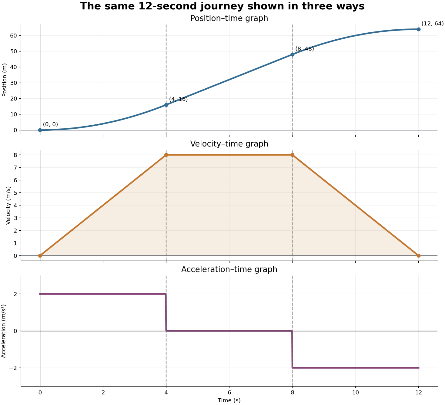
The three graphs show the same 12-second journey. The vertical dashed lines divide it into three stages.
Interpreting the example journey
The object begins from rest at a position of 0 m.
Its motion has three stages:
- From 0 to 4 seconds, it accelerates uniformly.
- From 4 to 8 seconds, it moves at constant velocity.
- From 8 to 12 seconds, it decelerates uniformly to rest.
Each graph describes these stages in a different way.
Stage 1: accelerating from rest
From 0 to 4 seconds, the acceleration is:
a = +2 m/s²
The area under the acceleration–time graph gives the change in velocity:
Δv = 2 × 4
Δv = 8 m/s
Because the initial velocity is zero:
v = 0 + 8
v = 8 m/s
On the velocity–time graph, velocity rises in a straight line from 0 to 8 m/s.
The area under this part of the velocity–time graph is a triangle:
Displacement = ½ × base × height
Displacement = ½ × 4 × 8
Displacement = 16 m
The position therefore increases from 0 m to 16 m.
On the position–time graph, the curve becomes progressively steeper. This shows that velocity is increasing.
Stage 2: moving at constant velocity
From 4 to 8 seconds, the velocity remains at:
v = 8 m/s
The horizontal velocity–time line has zero gradient, so:
a = 0 m/s²
The displacement is the rectangular area under the velocity–time graph:
Displacement = base × height
Displacement = 4 × 8
Displacement = 32 m
The object began this stage at 16 m:
Final position = 16 + 32
Final position = 48 m
On the position–time graph, this stage is a straight line. Its constant gradient represents constant velocity.
A velocity of 8 m/s does not require an acceleration of 8 m/s². An object can maintain a non-zero velocity while its acceleration is zero.
Stage 3: slowing to rest
From 8 to 12 seconds, velocity falls from 8 m/s to 0 m/s.
The acceleration is the gradient of the velocity–time graph:
a = (0 − 8) / (12 − 8)
a = −8 / 4
a = −2 m/s²
The negative acceleration acts opposite to the positive velocity, so the object slows down.
The displacement is the triangular area:
Displacement = ½ × 4 × 8
Displacement = 16 m
The object began this stage at 48 m:
Final position = 48 + 16
Final position = 64 m
The position–time graph gradually becomes less steep and ends horizontally. The horizontal tangent at 12 seconds shows that the final velocity is zero.
Finding total distance and displacement
All velocities in the example are positive. The object never reverses direction.
The total displacement equals the complete area under the velocity–time graph:
Displacement = 16 + 32 + 16
Displacement = 64 m
Because the object moves in only one direction:
Total distance = 64 m
If part of a velocity–time graph lies below the time axis, total distance and displacement must be handled differently.
- Displacement uses signed areas.
- Distance uses the magnitudes of all areas.
Finding average speed and average velocity
Average speed is:
Average speed = total distance ÷ total time
Average speed = 64 / 12
Average speed = 5.33 m/s
Average velocity is:
Average velocity = displacement ÷ total time
Average velocity = 64 / 12
Average velocity = 5.33 m/s in the positive direction
They are equal in this example because the object never changes direction.
If the object reversed direction, total distance would be greater than the magnitude of displacement.
Extracting values from gradients
A gradient measures the rate at which the vertical quantity changes relative to the horizontal quantity.
Gradient of a straight line
Choose two clear points that lie far apart:
Gradient = (y₂ − y₁) / (x₂ − x₁)
Using widely separated points generally reduces the effect of small reading errors.
Gradient of a curve
A curved graph has a changing gradient.
To estimate an instantaneous value:
- Locate the required point.
- Draw a tangent that touches the curve at that point.
- Choose two widely separated points on the tangent.
- Calculate the tangent’s gradient.
The chosen points should lie on the tangent. They do not have to lie on the original curve.
Worked example: velocity from a position graph
Between 4 and 8 seconds in the example:
v = (48 − 16) / (8 − 4)
v = 32 / 4
v = 8 m/s
This agrees with the velocity–time graph.
Extracting values from areas
The units of an area come from multiplying the units on the two axes.
For a velocity–time graph:
(m/s) × s = m
Therefore, the area represents displacement.
For an acceleration–time graph:
(m/s²) × s = m/s
Therefore, the area represents change in velocity.
Common area formulas
Rectangle
Area = base × height
Triangle
Area = ½ × base × perpendicular height
Trapezium
Area = ½ × (sum of parallel sides) × perpendicular distance
For a curved graph, the area may be estimated using strips or calculated using integration.
Worked example: motion involving a change of direction
A velocity–time graph shows:
- Velocity increases uniformly from 0 to 6 m/s during the first 3 seconds.
- Velocity decreases uniformly from 6 m/s at 3 seconds to −2 m/s at 7 seconds.
Find the acceleration from 3 to 7 seconds
a = [−2 − 6] / (7 − 3)
a = −8 / 4
a = −2 m/s²
Find when the object changes direction
The object changes direction when velocity crosses zero.
Starting at 6 m/s and decreasing at 2 m/s each second:
Time needed to reach zero = 6 / 2
Time needed = 3 s
This occurs 3 seconds after t = 3 s:
Direction changes at t = 6 s.
Find the displacement
From 0 to 3 seconds:
Area = ½ × 3 × 6
Area = 9 m
From 3 to 6 seconds:
Area = ½ × 3 × 6
Area = 9 m
From 6 to 7 seconds, the graph lies below the axis:
Signed area = −(½ × 1 × 2)
Signed area = −1 m
Total displacement:
9 + 9 − 1 = 17 m
Find the total distance
Use the magnitude of each area:
9 + 9 + 1 = 19 m
The displacement and distance differ because the object reverses direction.
Combining information from two graphs
Sometimes one graph does not contain enough information to answer a question.
Suppose an acceleration–time graph shows an acceleration of 3 m/s² for 5 seconds. The area gives:
Δv = 3 × 5
Δv = 15 m/s
This does not give the final velocity unless the initial velocity is known.
If a velocity–time graph or written statement shows an initial velocity of 4 m/s:
Final velocity = 4 + 15
Final velocity = 19 m/s
Similarly, the area under a velocity–time graph gives displacement. To find final position, add the initial position.
Comparing multiple objects
When two objects appear on the same graph, an intersection has a meaning determined by the vertical axis.
On a position–time graph
An intersection means the objects have the same position at the same time. They may meet or pass one another.
Their velocities may still be different. Compare the gradients at the intersection.
On a velocity–time graph
An intersection means the objects have the same velocity at the same time.
It does not show that they have the same position.
To determine whether they meet, compare their starting positions and accumulated displacements.
On an acceleration–time graph
An intersection means the objects have the same acceleration at that time.
It does not establish equal velocity or position.
Real-world example: analyzing a vehicle journey
A delivery van starts from a traffic light, travels along a straight road and stops at another light.
A velocity–time graph shows:
- 0–5 s: velocity rises uniformly from 0 to 10 m/s.
- 5–20 s: velocity remains at 10 m/s.
- 20–25 s: velocity falls uniformly to 0 m/s.
Acceleration during the first stage
a = (10 − 0) / 5
a = 2 m/s²
Acceleration during braking
a = (0 − 10) / 5
a = −2 m/s²
Total distance
First triangle:
½ × 5 × 10 = 25 m
Rectangle:
15 × 10 = 150 m
Final triangle:
½ × 5 × 10 = 25 m
Total distance:
25 + 150 + 25 = 200 m
Average speed
Average speed = 200 / 25
Average speed = 8 m/s
A strong written conclusion would be:
“The van travelled 200 m. This is the total area under the speed–time graph: two triangular areas of 25 m and a rectangular area of 150 m. Dividing by the 25-second journey time gives an average speed of 8 m/s.”
Explaining answers with graphical evidence
A complete graphical explanation should include:
- The relevant graph feature.
- The values read from the graph.
- The calculation or comparison.
- The correct units.
- A conclusion connected to the motion.
For example:
“The object accelerated at 2 m/s² from 0 to 4 seconds because the velocity–time graph rose from 0 to 8 m/s. Its gradient was (8 − 0)/(4 − 0) = 2 m/s².”
Avoid vague statements such as:
“The line goes up, so the object is faster.”
A rising line has different meanings on different graph types.
Checking whether an answer is reasonable
Use several checks before accepting an answer.
Check the units
- Position–time gradient: m/s.
- Velocity–time gradient: m/s².
- Velocity–time area: m.
- Acceleration–time area: m/s.
Check the sign
- Positive velocity: motion in the chosen positive direction.
- Negative velocity: motion in the opposite direction.
- Negative acceleration: acceleration in the negative direction.
A negative value does not automatically mean the object is slowing down.
Compare connected graphs
- Increasing velocity should match non-zero acceleration.
- Constant velocity should match zero acceleration.
- A stationary object should have a horizontal position–time graph.
- A position–time graph should become steeper as speed increases.
Check the scale
Do not assume each grid square represents one unit. Read labels carefully.
Check the physical context
A mathematical graph may continue beyond the period that makes sense physically. For example, a vehicle’s speed should not become negative unless it actually reverses direction.
Common misconceptions
- “The area under a position–time graph gives distance.” The gradient of a position–time graph gives velocity.
- “The gradient of a velocity–time graph gives velocity.” It gives acceleration.
- “A horizontal velocity–time line means the object is stationary.” It means constant velocity; the object is stationary only if that velocity is zero.
- “A line below the time axis means negative distance.” On a velocity graph, it represents motion in the negative direction.
- “Zero velocity means zero acceleration.” An object can have zero velocity at an instant while still accelerating.
- “An intersection always means two objects meet.” That interpretation applies to compatible position–time graphs.
- “Area gives the final value directly.” Area often gives a change, which must be combined with an initial value.
- “A steeper-looking graph always represents a greater rate.” Scales and units must be considered.
Did you know?
A position–time graph can be curved even when the acceleration is constant.
When acceleration is constant, velocity changes linearly with time. Since position accumulates that changing velocity, its graph becomes quadratic.
This is why the position–time graph in the main example curves during acceleration and deceleration, while the velocity–time graph consists of straight lines.
Key terms
- Position–time graph: A graph showing position relative to an origin as time changes.
- Velocity–time graph: A graph showing velocity as time changes.
- Acceleration–time graph: A graph showing acceleration as time changes.
- Gradient: Change in the vertical quantity divided by change in the horizontal quantity.
- Tangent: A line used to estimate a curve’s instantaneous gradient.
- Signed area: Area counted as positive above the time axis and negative below it.
- Displacement: Change in position, including direction.
- Distance: Total length of the path travelled.
- Instantaneous velocity: Velocity at a particular moment.
- Average velocity: Total displacement divided by total time.
- Change of direction: The event that occurs when velocity passes through zero and changes sign.
Key takeaways
- Begin by identifying the graph type, axes, scales and units.
- Position–time gradient gives velocity.
- Velocity–time gradient gives acceleration.
- Velocity–time area gives displacement.
- Acceleration–time area gives change in velocity.
- Add initial values when an area gives only a change.
- Separate positive and negative areas when calculating displacement or distance.
- Combine evidence from related graphs to check your interpretation.
- Support conclusions with graph values, calculations and units.