Applications of Probability and Combinatoric
| サイト: | Young Education |
| コース: | Probability and Combinatorics |
| ブック: | Applications of Probability and Combinatoric |
| 印刷者: | Guest user |
| 日付: | 2026年 11月 9日(月曜日) 16:38 |
1. Decision Making Under Uncertainty
Learning outcomes
- I can apply expected value to decision making.
- I can compare risks and rewards.
- I can analyse uncertain outcomes.
- I can evaluate alternative strategies.
- I can justify decisions mathematically.
Decision Making Under Uncertainty
Introduction to Decision Making Under Uncertainty
Every day, individuals, businesses, scientists, and governments make decisions without knowing exactly what will happen.
For example:
-
Should a company invest in a new product?
-
Is it better to repair an old machine or purchase a new one?
-
How much stock should a shop order when customer demand is uncertain?
-
Should a farmer plant a crop that produces higher profits but is more vulnerable to drought?
-
Which transportation option offers the best balance between cost, reliability, and travel time?
These decisions involve uncertainty, because several outcomes are possible and the final result cannot be predicted with certainty.
Mathematics provides methods for comparing these alternatives.
One of the most important tools is expected value, which combines possible outcomes with their probabilities to calculate a probability-weighted average.
However, a good decision may also depend on risk, the severity of possible losses, available resources, and the consequences of different outcomes.
Decision making under uncertainty involves using probability, expected value, and mathematical reasoning to compare alternatives and select an appropriate course of action.


Understanding Uncertainty and Risk
Although the words risk and uncertainty are often used together, they have slightly different meanings in decision analysis.
Risk describes situations where different outcomes are possible and their probabilities can be estimated.
Uncertainty is a broader term describing situations where the future is unknown. In some cases, even the probabilities of different outcomes may be difficult to estimate.
Examples
|
Situation |
Possible outcomes |
Source of uncertainty |
|---|---|---|
|
Launching a product |
High, moderate, or low sales |
Customer demand |
|
Planting crops |
High or low harvest |
Weather and growing conditions |
|
Purchasing equipment |
Reliable operation or breakdown |
Equipment performance |
|
Planning an event |
High or low attendance |
Customer participation |
|
Choosing transportation |
Early, on-time, or late arrival |
Traffic and service delays |
In many mathematical problems, probabilities are provided or can be estimated from data.
These probabilities allow us to calculate expected outcomes.
Expected Value
The expected value of a random variable is the probability-weighted average of its possible outcomes.
For a discrete random variable X:
E(X) = Σ[x × P(X = x)]
where:
-
E(X) is the expected value.
-
x is a possible numerical outcome.
-
P(X = x) is the probability of that outcome.
-
Σ means to add the products for all possible outcomes.
Interpretation
Expected value represents the long-run average outcome if the same decision or random experiment were repeated many times under the same conditions.
It does not necessarily represent an outcome that will actually occur.
For example, the expected number of heads in three fair coin tosses is 1.5.
However, obtaining exactly 1.5 heads is impossible.
Expected value is an average, not a guaranteed result.
Worked Example: Expected Profit
Suppose a company is considering launching a small product.
The possible profits are:
|
Outcome |
Probability |
Profit |
|---|---|---|
|
High sales |
0.30 |
$20,000 |
|
Moderate sales |
0.50 |
$8,000 |
|
Low sales |
0.20 |
−$5,000 |
A negative profit represents a loss.
Step 1: Multiply Each Outcome by Its Probability
High sales:
0.30 × $20,000 = $6,000
Moderate sales:
0.50 × $8,000 = $4,000
Low sales:
0.20 × (−$5,000) = −$1,000
Step 2: Add the Results
E(X) = $6,000 + $4,000 − $1,000
E(X) = $9,000
Interpretation
The expected profit is $9,000.
This does not mean the company will earn exactly $9,000.
The actual outcome could be a $20,000 profit, an $8,000 profit, or a $5,000 loss.
The expected value provides a mathematical summary of the possible outcomes and their probabilities.
Expected Monetary Value
When outcomes are measured in money, expected value is often called expected monetary value (EMV).
EMV = Σ[Probability × Monetary outcome]
EMV can be used to compare:
-
Investment opportunities.
-
Business strategies.
-
Equipment purchases.
-
Insurance decisions.
-
Product launches.
-
Project alternatives.
If the objective is to maximize expected monetary gain, the strategy with the highest EMV is preferred.
However, maximizing EMV does not always produce the most suitable decision when financial losses or other consequences are significant.
Comparing Alternative Strategies
Suppose a company is choosing between two business strategies.
Strategy A: Conservative Expansion
|
Outcome |
Probability |
Profit |
|---|---|---|
|
Successful expansion |
0.80 |
$12,000 |
|
Unsuccessful expansion |
0.20 |
−$2,000 |
Expected value:
EMV(A) = 0.80 × $12,000 + 0.20 × (−$2,000)
= $9,600 − $400
EMV(A) = $9,200
Strategy B: Aggressive Expansion
|
Outcome |
Probability |
Profit |
|---|---|---|
|
Successful expansion |
0.40 |
$30,000 |
|
Unsuccessful expansion |
0.60 |
−$4,000 |
Expected value:
EMV(B) = 0.40 × $30,000 + 0.60 × (−$4,000)
= $12,000 − $2,400
EMV(B) = $9,600
Comparing the Results
|
Measure |
Strategy A |
Strategy B |
|---|---|---|
|
Expected profit |
$9,200 |
$9,600 |
|
Maximum profit |
$12,000 |
$30,000 |
|
Maximum loss |
$2,000 |
$4,000 |
|
Probability of loss |
20% |
60% |
Strategy B has the higher expected profit.
However, it also has a higher probability of loss and a larger potential loss.
A company focused on maximizing expected profit may prefer Strategy B.
A company concerned about financial stability may prefer Strategy A.
The mathematically preferred decision depends on the objective and the constraints of the decision-maker.
Comparing Risks and Rewards
Expected value is important, but it does not fully describe risk.
Two strategies may have the same expected value while producing very different outcomes.
Example
Consider two options.
Option A
Receive $500 with certainty.
Expected value:
E(A) = $500
Option B
-
50% probability of receiving $1,200.
-
50% probability of losing $200.
Expected value:
E(B) = 0.50 × $1,200 + 0.50 × (−$200)
= $600 − $100
E(B) = $500
Both options have the same expected value.
However, Option A guarantees $500, while Option B involves substantial uncertainty.
Interpretation
A risk-averse person may prefer Option A.
A person willing to accept uncertainty for the possibility of a larger reward may prefer Option B.
Neither preference is automatically mathematically incorrect.
Expected value is only one part of the decision.
Variance and Standard Deviation in Decision Making
The variance of a random variable measures how widely possible outcomes are spread around the expected value.
For a discrete random variable:
Var(X) = Σ[(x − μ)² × P(X = x)]
where:
μ = E(X)
The standard deviation is:
σ = √Var(X)
A larger standard deviation indicates greater variability in possible outcomes.
Worked Example: Comparing Two Options
Consider the previous options.
Option A guarantees $500.
Therefore:
E(A) = $500
Var(A) = 0
σ(A) = 0
Option B offers:
-
$1,200 with probability 0.5.
-
−$200 with probability 0.5.
Its expected value is $500.
Calculate the variance:
Var(B) = 0.5 × (1200 − 500)² + 0.5 × (−200 − 500)²
= 0.5 × 700² + 0.5 × (−700)²
= 245,000 + 245,000
Var(B) = 490,000
Standard deviation:
σ(B) = √490000
σ(B) = $700
Interpretation
Both options have the same expected value, but Option B has a much larger standard deviation.
This means its possible outcomes vary more widely around the expected value.
Standard deviation provides a useful measure of risk when comparing outcomes on the same scale.
Decision Tables
A decision table, also called a payoff table, organizes possible decisions and their outcomes under different conditions.
Suppose a shop must decide how much stock to order.
The shop has two options:
-
Order 100 units.
-
Order 200 units.
Customer demand may be:
-
Low
-
High
The profits are:
|
Decision |
Low demand |
High demand |
|---|---|---|
|
Order 100 units |
$1,000 |
$1,000 |
|
Order 200 units |
−$500 |
$2,500 |
Suppose:
P(low demand) = 0.40
P(high demand) = 0.60
Expected Value of Ordering 100 Units
EMV(100) = 0.40 × $1,000 + 0.60 × $1,000
EMV(100) = $1,000
Expected Value of Ordering 200 Units
EMV(200) = 0.40 × (−$500) + 0.60 × $2,500
= −$200 + $1,500
EMV(200) = $1,300
Decision
Ordering 200 units has the higher expected profit.
However, ordering 100 units avoids the possibility of a loss under the two scenarios.
The appropriate decision depends on whether maximizing expected profit or limiting financial risk is more important.

Decision Trees
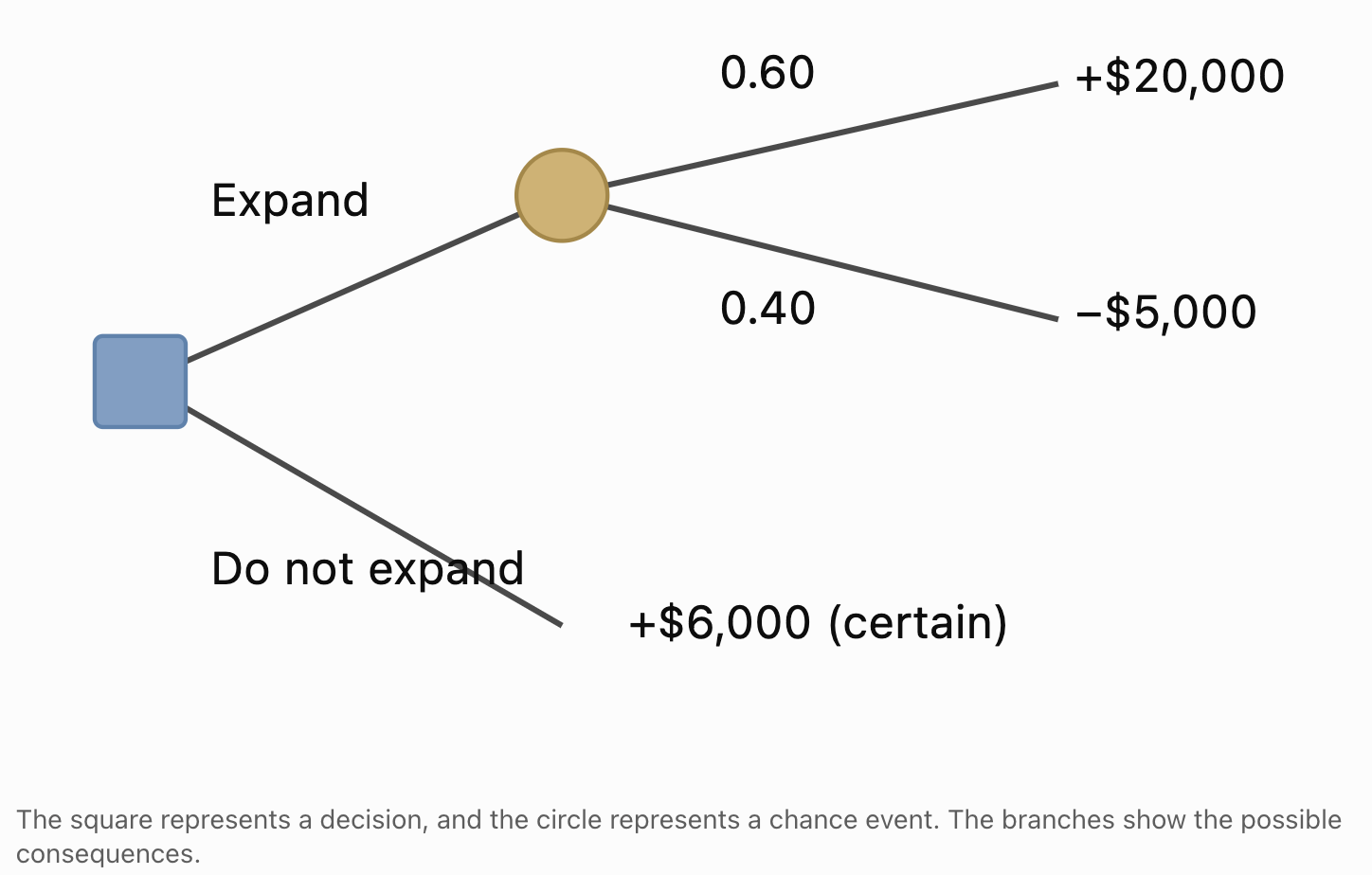
A decision tree is a diagram showing possible decisions, uncertain events, and their consequences.
Decision trees are useful when a problem involves several stages.
Two common types of nodes are:
-
Decision nodes: Points where a choice is made, often represented by squares.
-
Chance nodes: Points where an uncertain outcome occurs, often represented by circles.
Example: Business Expansion
A company must decide whether to expand.
If it expands:
-
There is a 60% probability of earning $20,000.
-
There is a 40% probability of losing $5,000.
If it does not expand:
- The profit is $6,000.
Step 1: Calculate the Expected Value of Expanding
EMV(expand) = 0.60 × $20,000 + 0.40 × (−$5,000)
= $12,000 − $2,000
EMV(expand) = $10,000
Step 2: Calculate the Value of Not Expanding
EMV(do not expand) = $6,000
Step 3: Compare
|
Decision |
Expected profit |
|---|---|
|
Expand |
$10,000 |
|
Do not expand |
$6,000 |
Expanding has the higher expected monetary value.
Decision
If the company wants to maximize expected profit and can tolerate the possible loss, expanding is the preferred strategy.
If avoiding losses is essential, not expanding may be more appropriate.
Analysing Decisions with Several Stages
Some decisions involve a sequence of uncertain events.
For example, a company might:
-
Invest in product development.
-
Conduct a market test.
-
Decide whether to launch the product.
-
Experience high or low customer demand.
Decision trees can represent these stages.
Solving Multi-Stage Decision Trees
A common method is rollback analysis.
Start at the final outcomes and work backward.
At each chance node:
Calculate the probability-weighted expected value.
At each decision node:
Choose the alternative with the preferred value according to the decision criterion.
Continue backward until reaching the initial decision.
This allows complex decisions to be evaluated systematically.
Risk Attitudes
People and organizations differ in how they respond to uncertain outcomes.
Three common attitudes toward risk are:
Risk-Averse
A risk-averse decision-maker prefers greater certainty when alternatives have the same expected value.
For example, they may prefer a guaranteed $500 over a risky option with an expected value of $500.
Risk-Neutral
A risk-neutral decision-maker evaluates alternatives primarily according to expected monetary value.
If two options have the same expected value, they are equally attractive under this criterion.
Risk-Seeking
A risk-seeking decision-maker may prefer an uncertain option over a guaranteed option with the same expected value.
The possibility of a large reward may be especially attractive.
Important Principle
Risk attitudes influence decisions, but they do not change the mathematical expected values of the alternatives.
Expected Utility
Expected monetary value is not always enough to describe preferences.
For example, losing $10,000 may have a very different impact on a small business than on a large corporation.
Utility is a mathematical representation of how desirable an outcome is to a decision-maker.
Expected utility is calculated using:
E[U(X)] = Σ[P(X = x) × U(x)]
where:
U(x) represents the utility of outcome x.
A decision-maker can compare alternatives using expected utility rather than expected money alone.
Example
A person may value financial security more highly than the possibility of earning a much larger amount.
A utility function can represent that preference.
Expected utility provides a more flexible framework for decision-making when risk attitudes matter.
The Value of Information
Sometimes a decision-maker can obtain additional information before making a decision.
For example:
-
A company might conduct market research.
-
A farmer might purchase a detailed weather forecast.
-
A manufacturer might inspect equipment.
-
A doctor might request an additional diagnostic test.
Information can improve decisions by reducing uncertainty.
Expected Value of Perfect Information
The expected value of perfect information (EVPI) measures how much better the expected outcome could be if the decision-maker knew the future state before choosing.
EVPI = Expected value with perfect information − Best expected value without perfect information
EVPI represents the maximum amount a risk-neutral decision-maker should be willing to pay for perfect information under the model.
Worked Example: Value of Market Research
Consider the earlier stock-ordering problem.
|
Decision |
Low demand |
High demand |
|---|---|---|
|
Order 100 units |
$1,000 |
$1,000 |
|
Order 200 units |
−$500 |
$2,500 |
Probabilities:
P(low demand) = 0.40
P(high demand) = 0.60
The best expected value without additional information is:
$1,300
With Perfect Information
If the shop knew demand would be low, it would order 100 units and earn $1,000.
If it knew demand would be high, it would order 200 units and earn $2,500.
Expected value with perfect information:
EV(with perfect information) = 0.40 × $1,000 + 0.60 × $2,500
= $400 + $1,500
= $1,900
Calculate EVPI
EVPI = $1,900 − $1,300
EVPI = $600
Interpretation
Perfect information would increase expected profit by $600.
Therefore, under this model, a risk-neutral shop owner should not pay more than $600 for perfect information.
Real market research is imperfect, so its expected value would generally be lower.
Decisions When Probabilities Are Unknown
Sometimes probabilities cannot be estimated reliably.
In these situations, expected value may not be appropriate.
Alternative decision criteria can be used.
Maximax Criterion
Choose the strategy with the highest possible payoff.
This is an optimistic approach.
Maximin Criterion
Choose the strategy with the highest worst-case payoff.
This is a conservative approach.
Minimax Regret Criterion
Choose the strategy that minimizes the largest possible regret.
Regret is the difference between the best payoff that could have been obtained in a particular state and the payoff from the chosen strategy.
Example
|
Strategy |
Low demand |
High demand |
|---|---|---|
|
A |
$5,000 |
$10,000 |
|
B |
−$2,000 |
$20,000 |
|
C |
$3,000 |
$14,000 |
Maximax: Strategy B, because its maximum payoff is $20,000.
Maximin: Strategy A, because its minimum payoff is $5,000, higher than the minimum payoffs of the other strategies.
For minimax regret:
-
Under low demand, the best payoff is $5,000.
-
Under high demand, the best payoff is $20,000.
|
Strategy |
Regret under low demand |
Regret under high demand |
Maximum regret |
|---|---|---|---|
|
A |
$0 |
$10,000 |
$10,000 |
|
B |
$7,000 |
$0 |
$7,000 |
|
C |
$2,000 |
$6,000 |
$6,000 |
Minimax regret: Strategy C, because its maximum regret is the smallest.
Different decision criteria can produce different choices.
Sensitivity Analysis in Decision Making
Decision models depend on estimated probabilities.
If these probabilities change, the preferred strategy may also change.
Sensitivity analysis examines how changes in assumptions affect the decision.
Worked Example
Suppose a company is considering a project.
If successful, the project earns $15,000.
If unsuccessful, it loses $5,000.
Let p be the probability of success.
Expected value:
EMV = 15000p − 5000(1 − p)
Expand:
EMV = 15000p − 5000 + 5000p
EMV = 20000p − 5000
Find the Break-Even Probability
Set expected value equal to zero:
20000p − 5000 = 0
20000p = 5000
p = 0.25
Interpretation
-
If p > 0.25, the expected profit is positive.
-
If p = 0.25, the expected profit is zero.
-
If p < 0.25, the expected profit is negative.
The break-even success probability is 25%.
This result helps the company evaluate whether its estimate of the probability of success is sufficiently high.
Comparing Strategies Across Different Probabilities
Using the previous example:
EMV = 20000p − 5000
|
Probability of success |
Expected profit |
|---|---|
|
10% |
−$3,000 |
|
20% |
−$1,000 |
|
25% |
$0 |
|
40% |
$3,000 |
|
60% |
$7,000 |
|
80% |
$11,000 |
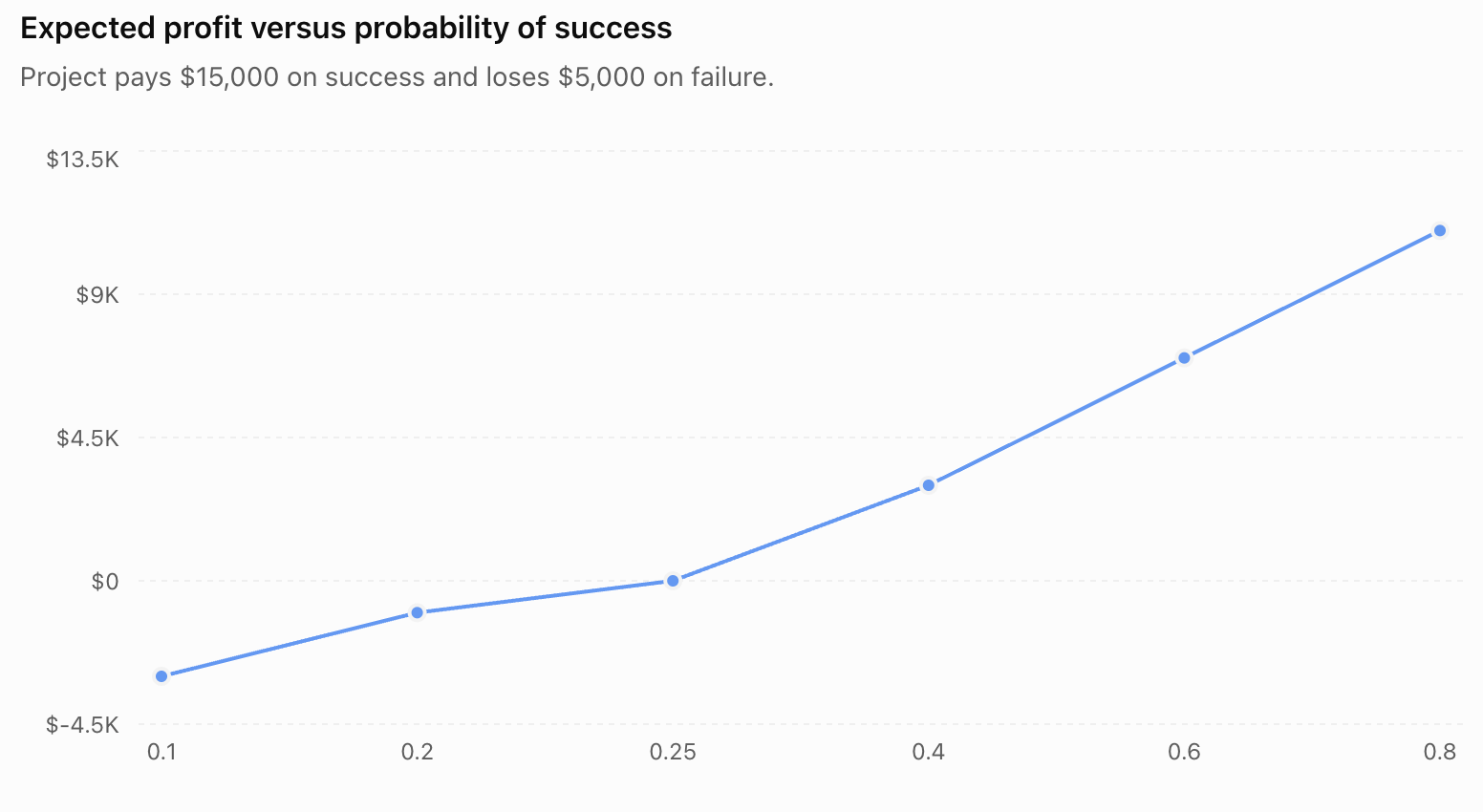
The graph illustrates how the expected profit increases as the probability of success increases.
Sensitivity analysis is especially useful when probabilities are uncertain or based on limited data.
Practical Application: Equipment Replacement
A factory must decide whether to continue using an older machine or purchase a replacement.
Keep the Old Machine
-
70% probability of no major breakdown, costing $2,000 in maintenance.
-
30% probability of a breakdown, costing $18,000 in total.
Expected cost:
E(C_old) = 0.70 × $2,000 + 0.30 × $18,000
= $1,400 + $5,400
E(C_old) = $6,800
Purchase a New Machine
Suppose the new machine has a total annualized cost of $6,000, including purchase-related costs and expected maintenance.
Expected cost:
E(C_new) = $6,000
Decision
|
Option |
Expected cost |
|---|---|
|
Keep old machine |
$6,800 |
|
Purchase new machine |
$6,000 |
Purchasing the new machine has the lower expected cost by $800.
However, the company should also consider equipment lifespan, downtime, productivity, and the accuracy of the cost estimates.

Practical Application: Agricultural Decisions
A farmer must choose between two crops.
Crop A produces relatively stable profits.
Crop B can produce much higher profits in favourable weather but performs poorly during drought.
Suppose:
|
Weather |
Probability |
Crop A profit |
Crop B profit |
|---|---|---|---|
|
Good rainfall |
0.60 |
$12,000 |
$20,000 |
|
Drought |
0.40 |
$6,000 |
−$4,000 |
Expected Profit for Crop A
EMV(A) = 0.60 × $12,000 + 0.40 × $6,000
= $7,200 + $2,400
EMV(A) = $9,600
Expected Profit for Crop B
EMV(B) = 0.60 × $20,000 + 0.40 × (−$4,000)
= $12,000 − $1,600
EMV(B) = $10,400
Crop B has the higher expected profit.
However, Crop A provides a positive profit under both weather conditions.
A farmer with limited financial reserves may reasonably prefer Crop A.

Practical Application: Transportation Choices
Suppose a student can travel to school using either a bus or a train.
Bus
-
70% probability of arriving in 25 minutes.
-
30% probability of arriving in 45 minutes.
Expected travel time:
E(T_bus) = 0.70 × 25 + 0.30 × 45
= 17.5 + 13.5
E(T_bus) = 31 minutes
Train
-
90% probability of arriving in 30 minutes.
-
10% probability of arriving in 40 minutes.
Expected travel time:
E(T_train) = 0.90 × 30 + 0.10 × 40
= 27 + 4
E(T_train) = 31 minutes
Both options have the same expected travel time.
However, the train has less variation in travel time.
A student who must arrive before a strict deadline may prefer the train.
This example demonstrates why expected value alone may not determine the best choice.
Communicating Mathematical Decisions
A well-justified decision should explain both the calculations and the reasoning behind the recommendation.
A Strong Mathematical Justification Includes
-
A clear statement of the decision.
-
The available alternatives.
-
Possible outcomes and their probabilities.
-
Expected value calculations.
-
Relevant measures of risk.
-
Assumptions and limitations.
-
A conclusion that matches the decision objective.
Example
"Strategy B has an expected profit of $9,600, compared with $9,200 for Strategy A. Therefore, Strategy B is preferable if the objective is to maximize expected profit. However, Strategy B also has a 60% probability of loss, compared with 20% for Strategy A. A company prioritizing financial stability may therefore prefer Strategy A despite its slightly lower expected value."
This explanation is stronger than simply stating that Strategy B is better.
It recognises both expected reward and risk.
Limitations of Mathematical Decision Models
Mathematical models help organize uncertain decisions, but they have limitations.
Estimated Probabilities May Be Incorrect
Probabilities are often based on historical data or assumptions.
Future conditions may differ from the past.
Outcomes May Be Incomplete
Some important consequences may be difficult to measure financially.
For example:
-
Environmental damage.
-
Safety risks.
-
Reputation.
-
Customer satisfaction.
-
Social consequences.
Decision-Makers Have Different Objectives
One person may prioritize maximum expected profit.
Another may prioritize avoiding severe losses.
Rare Events Can Have Major Consequences
An event with a small probability may still require serious attention if its consequences are extremely harmful.
Conditions May Change
Market demand, weather, technology, and other factors can change over time.
Decision models should be reviewed when new information becomes available.
Common Mistakes
Assuming the highest expected value is always the best decision
Expected value does not fully describe risk, financial constraints, or personal preferences.
Ignoring negative outcomes
Losses must be included using negative values when calculating expected profit.
Forgetting to multiply outcomes by probabilities
Expected value is a weighted average, not a simple average unless outcomes are equally likely.
Using probabilities that do not add to 1
A complete probability distribution must have total probability equal to 1.
Confusing expected value with a guaranteed outcome
The expected value may never occur in a single trial.
Ignoring the probability of severe losses
A strategy may have a high expected value while exposing the decision-maker to unacceptable risks.
Confusing variance and standard deviation
Variance is measured in squared units, while standard deviation uses the original units.
Comparing costs and profits incorrectly
When evaluating profits, larger expected values are generally preferred. When evaluating costs, smaller expected values are generally preferred.
Assuming perfect information is free
Obtaining information may involve financial costs and delays.
Failing to consider uncertain probabilities
Sensitivity analysis is important when probability estimates may be inaccurate.
Providing a decision without mathematical justification
A strong conclusion should include calculations, assumptions, and interpretation.
Key Terms
-
Decision Making Under Uncertainty: Choosing between alternatives when future outcomes are not known with certainty.
-
Risk: Exposure to uncertain outcomes whose probabilities can be estimated.
-
Uncertainty: Lack of certainty about future events or outcomes.
-
Expected Value: The probability-weighted average of possible numerical outcomes.
-
Expected Monetary Value (EMV): Expected value when outcomes are expressed in money.
-
Payoff: The result or reward associated with a decision and a particular outcome.
-
Payoff Table: A table organizing possible decisions and their outcomes.
-
Decision Tree: A diagram representing decisions, uncertain events, and possible consequences.
-
Decision Node: A point in a decision tree where a choice must be made.
-
Chance Node: A point in a decision tree where an uncertain event occurs.
-
Rollback Analysis: A method of solving decision trees by working backward from final outcomes.
-
Variance: A measure of how widely possible outcomes are spread around their expected value.
-
Standard Deviation: The square root of variance, measuring variability in the original units.
-
Risk-Averse: Preferring greater certainty when alternatives have the same expected value.
-
Risk-Neutral: Evaluating alternatives primarily according to expected monetary value.
-
Risk-Seeking: Preferring greater uncertainty when alternatives have the same expected value.
-
Utility: A numerical representation of how desirable an outcome is to a decision-maker.
-
Expected Utility: The probability-weighted average of the utilities of possible outcomes.
-
Value of Information: The improvement in expected decision outcomes made possible by additional information.
-
Expected Value of Perfect Information (EVPI): The maximum expected improvement achievable by knowing the future state before making a decision.
-
Maximax Criterion: A decision rule that selects the alternative with the highest possible payoff.
-
Maximin Criterion: A decision rule that selects the alternative with the highest worst-case payoff.
-
Minimax Regret: A decision rule that minimizes the largest possible regret.
-
Regret: The difference between the best available payoff in a particular state and the payoff from the selected strategy.
-
Sensitivity Analysis: An investigation of how changes in assumptions affect decision outcomes.
-
Break-Even Probability: The probability at which an expected payoff or the difference between strategies reaches zero.
-
Opportunity Cost: The value of the best alternative forgone when a decision is made.
-
Mathematical Justification: An explanation supporting a decision using calculations, assumptions, and logical reasoning.
Key Takeaways
-
Expected value is a powerful tool for comparing decisions involving uncertain outcomes.
-
Expected value is calculated by multiplying each possible outcome by its probability and adding the results.
-
Expected monetary value applies expected value to financial decisions.
-
A higher expected value does not guarantee a better outcome in any single situation.
-
Expected value represents a long-run average under the assumptions of the model.
-
Risk and reward should be considered together.
-
Variance and standard deviation measure the variability of possible outcomes.
-
Two alternatives can have the same expected value but different levels of risk.
-
Decision tables organize alternative strategies and possible outcomes.
-
Decision trees represent sequences of decisions and uncertain events.
-
Rollback analysis evaluates multi-stage decisions by working backward.
-
Risk-averse, risk-neutral, and risk-seeking decision-makers may prefer different strategies.
-
Expected utility can represent preferences that expected monetary value alone does not capture.
-
Additional information can improve decisions by reducing uncertainty.
-
EVPI measures the maximum expected benefit of perfect information.
-
When probabilities are unknown, maximax, maximin, and minimax regret provide alternative decision criteria.
-
Sensitivity analysis shows how changes in probabilities affect expected outcomes.
-
Break-even probabilities identify thresholds where a decision becomes financially favourable.
-
Mathematical decisions should consider assumptions, limitations, and possible consequences.
-
A strong mathematical justification explains the calculations and why the recommended strategy fits the decision objective.
Check Your Understanding
Recall and Understanding
-
Define expected value and explain how it is used in decision making.
-
Explain the difference between risk and uncertainty.
-
Describe the purpose of a decision tree.
-
Explain why two strategies with the same expected value may not be equally attractive.
-
Distinguish between risk-averse, risk-neutral, and risk-seeking decision-makers.
Application
-
A project has a 60% probability of earning $10,000 and a 40% probability of losing $3,000. Calculate its expected monetary value.
-
Strategy A guarantees a profit of $4,000. Strategy B offers a 50% probability of earning $10,000 and a 50% probability of losing $1,000. Compare their expected values.
-
A company can purchase a machine with an expected annual operating cost of $5,000 or keep an older machine with a 70% probability of costing $3,000 and a 30% probability of costing $12,000. Determine which option has the lower expected cost.
-
A decision has two outcomes: a $2,000 profit with probability 0.8 and a $3,000 loss with probability 0.2. Calculate the expected value and standard deviation.
-
A project earns $8,000 if successful and loses $2,000 if unsuccessful. Find the minimum probability of success required for a positive expected profit.
Analysis and Challenge
-
A company must choose between two strategies. Strategy A has an expected profit of $15,000 and a standard deviation of $2,000. Strategy B has an expected profit of $18,000 and a standard deviation of $10,000. Explain which strategy may be preferable for different risk attitudes.
-
A shop can order either 50 or 100 products. Construct a payoff table using reasonable assumptions about demand, calculate expected profits, and justify the preferred order quantity.
-
A business can conduct market research before launching a product. Explain how the expected value of perfect information could help determine whether the research is worth purchasing.
-
A project has a 40% probability of earning $20,000 and a 60% probability of losing $5,000. Calculate its expected value. Then explain how the decision might change if the probability of success were uncertain.
-
Design a real-world decision problem involving at least three possible outcomes and two alternative strategies. Construct a payoff table, calculate expected values, compare risks, and justify your recommended decision.
Final Summary
Decision making under uncertainty involves selecting between alternatives when future outcomes cannot be predicted with certainty.
Expected value provides a mathematical method for comparing strategies by combining possible outcomes with their probabilities.
However, expected value alone does not describe the full range of possible consequences.
Measures such as variance and standard deviation help quantify risk, while decision trees, payoff tables, and sensitivity analysis provide additional tools for evaluating alternatives.
Different decision-makers may choose different strategies because they have different objectives, resources, and attitudes toward risk.
The most effective decisions combine mathematical calculations with careful consideration of assumptions, uncertainty, and practical consequences.
A well-justified decision is not simply the one with the highest expected value. It is the decision that best meets the objective while accounting for the risks and limitations of the available information.
2. Games of Chance
Learning outcomes
- I can analyse lotteries and gambling games.
- I can calculate fair payouts.
- I can determine house advantage.
- I can evaluate gambling strategies mathematically.
- I can interpret long-term expected outcomes.
Games of Chance
Introduction to Games of Chance
Games of chance are activities in which outcomes depend partly or entirely on random events. Examples include lotteries, dice games, card games, roulette, and prize draws.
Although individual outcomes are uncertain, mathematics allows us to analyse how these games work.
Probability can help answer important questions:
-
What is the probability of winning?
-
How much should a fair game pay?
-
What is the expected profit or loss from playing?
-
How do gambling operators make money?
-
Can a betting strategy change the expected outcome?
-
What happens when a game is repeated many times?
The key mathematical concepts are probability, expected value, fair payouts, house advantage, and long-term outcomes.
Understanding these concepts allows us to evaluate games of chance objectively and distinguish between short-term luck and long-term mathematical expectations.


Understanding Games of Chance
A game of chance is a game in which randomness affects the result.
Some games depend almost entirely on chance, while others combine chance with skill.
Examples include:
|
Game |
Main source of uncertainty |
|---|---|
|
Lottery |
Random selection of numbers |
|
Roulette |
Random location of the ball |
|
Dice game |
Results of dice rolls |
|
Prize draw |
Random selection of a winner |
|
Card game |
Random distribution of cards |
|
Slot machine |
Randomly determined symbol combinations |
To analyse a game mathematically, we must identify:
-
The possible outcomes.
-
The probability of each outcome.
-
The cost of playing.
-
The payout associated with each outcome.
-
The player's net gain or loss.
Gross Payout Versus Net Profit
These two quantities must be distinguished.
Gross payout is the amount received when a prize is awarded.
Net profit is the payout minus the cost of playing.
For example, if a ticket costs $5 and pays $20:
Net profit = $20 − $5
Net profit = $15
If the ticket does not win:
Net profit = $0 − $5
Net profit = −$5
This distinction is essential when calculating expected value.
Expected Value in Games of Chance
Expected value measures the probability-weighted average of possible outcomes.
For a discrete random variable X:
E(X) = Σ[x × P(X = x)]
where:
-
E(X) is the expected value.
-
x is a possible outcome.
-
P(X = x) is the probability of that outcome.
-
Σ means to add all the probability-weighted outcomes.
For games of chance, X often represents the player's net profit.
Interpretation
If a game has an expected value of −$2 per play, the player is expected to lose an average of $2 per play over a very large number of repetitions.
This does not mean the player loses exactly $2 every time.
Some plays may produce large wins, while others produce losses.
Expected value describes the long-term mathematical average.
Worked Example: A Simple Dice Game
A player pays $3 to roll a fair six-sided die.
If the die shows a 6, the player receives $12.
Otherwise, the player receives nothing.
Step 1: Identify the Probabilities
P(rolling a 6) = 1/6
P(not rolling a 6) = 5/6
Step 2: Determine Net Outcomes
If the player wins:
Net profit = $12 − $3 = $9
If the player loses:
Net profit = −$3
Step 3: Calculate Expected Value
E(X) = (1/6 × $9) + (5/6 × −$3)
= $1.50 − $2.50
E(X) = −$1
Interpretation
The player loses an average of $1 per game in the long run.
The game favours the operator.
Fair Games
A fair game is a game in which the expected net profit is zero.
E(X) = 0
In a fair game, neither the player nor the operator has a mathematical advantage in expected monetary value.
Example: Fair Coin-Toss Game
A player pays $5 to play.
A fair coin is tossed.
If heads appears, the player receives $10.
If tails appears, the player receives nothing.
The possible net outcomes are:
|
Outcome |
Probability |
Net profit |
|---|---|---|
|
Heads |
0.5 |
+$5 |
|
Tails |
0.5 |
−$5 |
Expected value:
E(X) = 0.5 × $5 + 0.5 × (−$5)
= $2.50 − $2.50
E(X) = $0
The game is fair in terms of expected monetary value.
Important Distinction
A fair game does not guarantee that each player breaks even.
Individual players can still win or lose.
Fairness refers to the mathematical expectation over repeated plays.
Calculating Fair Payouts
A fair payout is the prize amount that makes the expected net profit equal to zero.
Suppose a game costs $4 to play.
The probability of winning is 1/8.
The player receives a gross payout of W dollars if successful and nothing otherwise.
Step 1: Construct the Expected Value Equation
E(X) = (1/8)(W − 4) + (7/8)(−4)
For a fair game:
E(X) = 0
Step 2: Solve
0 = (W − 4)/8 − 28/8
0 = (W − 32)/8
W = $32
Interpretation
The fair gross payout is $32.
The player's net profit when winning would be:
$32 − $4 = $28
The probability of winning is 1/8, so the expected gross payout is:
1/8 × $32 = $4
This exactly equals the cost of playing.
General Formula for a Fair Payout
Suppose:
-
The game costs C dollars.
-
The probability of winning is p.
-
The winner receives a gross payout W.
-
All other outcomes pay nothing.
The expected net profit is:
E(X) = pW − C
For a fair game:
0 = pW − C
Therefore:
W = C/p
Example
A lottery ticket costs $2.
The probability of winning is 1/500.
The fair gross payout is:
W = 2/(1/500)
W = $1,000
A gross prize of $1,000 would make this simplified lottery fair, assuming there are no other prizes or costs.
Fair Odds
Fair odds describe the relationship between the probability of winning and the payout required for a fair game.
Suppose an event has probability p.
The fair gross payout multiplier per unit staked is:
1/p
The fair net profit multiplier on a winning bet is:
(1 − p)/p
Example
An event has probability:
p = 0.20
Fair gross payout multiplier:
1/0.20 = 5
For a $10 stake:
Fair gross payout = $50
Fair net profit if successful:
$50 − $10 = $40
The fair net odds are 4 to 1.
Important Distinction
A quoted payout may refer to the total amount returned or only the profit.
Always determine whether the original stake is included.
Lotteries and Combinations
Lotteries often involve selecting several numbers from a larger set.
Combinations are useful when the order of selection does not matter.
The number of ways to select r objects from n objects is:
C(n,r) = n!/[r!(n − r)!]
where ! represents factorial.
Worked Example: A Six-Number Lottery
Suppose a lottery requires selecting six numbers from 49.
The order of the selected numbers does not matter.
The number of possible combinations is:
C(49,6) = 49!/(6!43!)
C(49,6) = 13,983,816
If one combination wins the jackpot:
P(jackpot) = 1/13,983,816
This is approximately:
0.00000715%
The probability of winning is extremely small.

Calculating a Fair Lottery Jackpot
Suppose the six-number lottery costs $2 per ticket.
There is only one prize: the jackpot.
The probability of winning is:
p = 1/13,983,816
The fair gross payout is:
W = C/p
W = 2 × 13,983,816
W = $27,967,632
Under this simplified model, a jackpot of approximately $27.97 million would make the expected net value of a ticket zero.
Important Limitations
Real lotteries often include:
-
Multiple prize categories.
-
Shared jackpots.
-
Taxes.
-
Administrative costs.
-
Different ticket prices.
-
Jackpot rollover rules.
These factors affect the expected value.
A jackpot larger than the simple fair amount does not necessarily make a real lottery favourable, especially when the prize may be shared among several winners.
House Advantage
The house advantage, also called the house edge, measures the operator's expected profit as a percentage of the player's stake.
For a game with stake C:
House edge = −E(player net profit)/C × 100%
This assumes the game is analysed from the player's perspective.
Example
Suppose a game costs $10 to play.
The expected net profit for the player is:
E(X) = −$0.80
Then:
House edge = −(−0.80)/10 × 100%
House edge = 8%
Interpretation
The operator expects to earn an average of 8% of the amount wagered over many plays.
This does not mean the operator earns exactly 8% from every player or every game.
Actual results vary because of randomness.
Roulette and House Advantage
Roulette provides a useful example of how the house edge is created.
In European roulette, there are 37 numbered pockets:
0 through 36.
Suppose a player places a $1 bet on one specific number.
The probability of winning is:
P(win) = 1/37
The probability of losing is:
P(loss) = 36/37
A winning straight-up bet pays 35 to 1 in net profit, with the original $1 stake also returned.
Expected Value
E(X) = (1/37 × $35) + (36/37 × −$1)
= 35/37 − 36/37
E(X) = −$1/37 ≈ −$0.0270
House Edge
House edge = (1/37) × 100%
≈ 2.70%
The house advantage comes from the difference between the fair payout and the actual payout.
Fair Payout Comparison
The fair net profit on a $1 straight-up winning bet would be $36.
The actual net profit is $35.
That difference creates the house edge.

Comparing European and American Roulette
European roulette contains 37 pockets.
American roulette usually contains 38 pockets because it has both 0 and 00.
For a straight-up bet paying 35 to 1:
|
Feature |
European roulette |
American roulette |
|---|---|---|
|
Number of pockets |
37 |
38 |
|
Winning probability |
1/37 |
1/38 |
|
Net profit on a $1 winning bet |
$35 |
$35 |
|
House edge |
2.70% |
5.26% |
American Roulette Calculation
E(X) = (1/38 × $35) + (37/38 × −$1)
= −2/38
≈ −$0.0526
House edge:
≈ 5.26%
American roulette has a higher house advantage because of the additional pocket.
These figures assume standard straight-up bets and payouts.
Return to Player
Another way to describe gambling mathematics is return to player (RTP).
RTP represents the expected proportion of wagers returned to players as gross payouts over the long run.
RTP = Expected gross payout / Stake × 100%
For a game where all stakes are accounted for through payouts and operator profit:
RTP = 100% − House edge
Example
If a game has a house edge of 4%:
RTP = 100% − 4%
RTP = 96%
This means that, on average, the game returns $96 in gross payouts for every $100 wagered over a very large number of plays.
It does not mean a player who wagers $100 will necessarily receive $96.
Long-Term Expected Outcomes
Expected value becomes particularly important when a game is repeated many times.
Suppose a game has an expected loss of $0.50 per play.
If a player participates in n games, the expected total net profit is:
E(total profit) = n × E(profit per game)
This follows from the linearity of expectation and does not require independence, provided the expected value per play remains the same.
Example
Expected loss per game:
−$0.50
After 100 games:
E(total) = 100 × (−$0.50)
= −$50
After 1,000 games:
E(total) = 1,000 × (−$0.50)
= −$500
After 10,000 games:
E(total) = 10,000 × (−$0.50)
= −$5,000
The expected total loss grows with the amount of play.
The Law of Large Numbers
The Law of Large Numbers helps explain long-term behaviour in games of chance.
Under suitable conditions, the average result of many repeated independent games approaches the expected value.
For example, suppose a game has an expected loss of $0.20 per play.
After a small number of plays, the player's average result may be positive or negative.
After many plays, the average result per game tends toward −$0.20.
Important Distinction
The Law of Large Numbers does not guarantee that every player loses exactly the expected amount.
A player can experience a long winning streak.
However, repeated play does not change a negative expected value into a positive one.
Short-Term Luck Versus Long-Term Expectation
Consider a game in which a player:
-
Wins $9 with probability 0.1.
-
Loses $1 with probability 0.9.
Expected value:
E(X) = 0.1 × $9 + 0.9 × (−$1)
= $0.90 − $0.90
E(X) = $0
This is a fair game.
However, the results of ten plays may vary considerably.
One player might win three times and lose seven times:
Total profit = 3 × $9 − 7 × $1
= $20
Another player might lose all ten games:
Total profit = −$10
Both outcomes are possible even though the expected value is zero.
This demonstrates the difference between expected value and actual results.
Variance and Volatility in Games
Expected value describes the average outcome, but it does not describe how widely results can vary.
Variance and standard deviation measure this variability.
For a discrete random variable:
Var(X) = Σ[(x − μ)² × P(X = x)]
where:
μ = E(X)
Standard deviation:
σ = √Var(X)
Example: Two Fair Games
Game A:
-
50% chance of winning $1.
-
50% chance of losing $1.
Game B:
-
50% chance of winning $100.
-
50% chance of losing $100.
Both games have expected value zero.
However:
Game A has standard deviation $1.
Game B has standard deviation $100.
Game B has much greater variability and financial risk.
A fair game can still involve substantial losses.
Evaluating Gambling Strategies
Players sometimes use betting systems in an attempt to overcome the house advantage.
A common misconception is that changing the size or sequence of bets can turn a negative-expectation game into a profitable one.
However, if each wager has the same negative expected return per dollar, changing bet sizes does not remove the underlying disadvantage.
Example
Suppose a game has a house edge of 5%.
For a $10 wager:
Expected loss = $0.50
For a $100 wager:
Expected loss = $5
For a total of $1,000 wagered:
Expected loss = $50
Changing the distribution of wagers does not remove the expected loss associated with the total amount staked, assuming the same house edge applies.
The Martingale Strategy
The Martingale strategy is a betting system in which a player doubles the wager after each loss.
The idea is that a future win will recover earlier losses and produce a small profit.
Consider a simplified even-money game with a probability of winning slightly below 50%.
A player begins with a $1 bet.
After each loss, the next wager doubles.
|
Consecutive losses before next bet |
Next wager |
Total already lost |
|---|---|---|
|
0 |
$1 |
$0 |
|
1 |
$2 |
$1 |
|
2 |
$4 |
$3 |
|
3 |
$8 |
$7 |
|
4 |
$16 |
$15 |
|
5 |
$32 |
$31 |
|
6 |
$64 |
$63 |
The required wager increases rapidly.
Mathematical Problem
After k consecutive losses:
Next wager = 2ᵏ × Initial wager
The total amount lost is:
Total losses = (2ᵏ − 1) × Initial wager
After ten consecutive losses with a $1 initial wager:
Total losses = 2¹⁰ − 1
= $1,023
The next required wager would be:
$1,024
Why the Strategy Fails to Remove the House Edge
The strategy does not change the probability of winning an individual independent bet.
It also introduces substantial risks:
-
Large wagers may be required.
-
Players have limited funds.
-
Games may have betting limits.
-
Long losing sequences remain possible.
-
A single losing sequence can erase many small gains.
The Martingale system changes the distribution of gains and losses but does not eliminate a negative expected value.
The Gambler's Fallacy
The gambler's fallacy is the mistaken belief that previous independent outcomes influence future probabilities.
Example: Coin Tosses
Suppose a fair coin produces heads five times in a row.
A player might believe that tails is now more likely.
However:
P(Tails on next toss) = 0.5
The probability remains unchanged.
Each toss is independent.
Roulette Example
Suppose a roulette wheel produces red several times in succession.
This does not make black more likely on the next spin, assuming independent spins and an unchanged wheel.
Past outcomes do not create a mathematical obligation for future outcomes to balance them.
Important Principle
Random processes do not compensate for previous outcomes simply because a particular result has occurred frequently or infrequently.
Hot Numbers and Cold Numbers
Some lottery players select numbers based on previous results.
A number that has appeared frequently may be called a hot number.
A number that has appeared infrequently may be called a cold number.
In a properly randomized lottery with independent draws:
-
Previous appearances do not increase a number's probability.
-
Previous absences do not increase a number's probability.
-
Every valid combination has the same probability of being selected.
For example, the combination:
1, 2, 3, 4, 5, 6
has the same probability of being selected as any other specific six-number combination in a fair six-from-49 lottery.
Although one combination may look more unusual than another, their individual probabilities are equal.
Can Skill Change the Expected Value?
Not all gambling-related games are purely random.
Some games involve decisions that affect the probabilities or payouts.
For example:
-
Certain card games involve strategic decisions.
-
Some competitions involve both skill and chance.
-
Promotional offers may change the effective cost of participation.
In these situations, mathematical analysis may need to account for the player's decisions and the rules of the game.
However, the existence of skill does not automatically imply a positive expected value.
The relevant probabilities, costs, and payouts must still be evaluated.
Practical Application: Prize Draws
Suppose a school organizes a fundraising prize draw.
There are 500 tickets.
Each ticket costs $4.
One ticket wins a prize worth $1,000.
Probability of Winning
P(win) = 1/500
Expected Gross Prize Value
E(gross prize) = 1/500 × $1,000
= $2
Expected Net Value
E(net) = $2 − $4
= −$2
The expected monetary loss per ticket is $2.
House Advantage
House edge = $2/$4 × 100%
= 50%
Interpretation
From a purely financial perspective, the ticket has a negative expected value.
However, participants may purchase tickets to support the school rather than to maximize financial return.
This illustrates how the purpose of an activity can influence how its value is interpreted.

Comparing Games Mathematically
Suppose three games each cost $5.
|
Game |
Winning probability |
Gross prize |
|---|---|---|
|
A |
1/2 |
$8 |
|
B |
1/5 |
$20 |
|
C |
1/10 |
$40 |
Game A
Expected gross payout:
1/2 × $8 = $4
Expected net profit:
$4 − $5 = −$1
House edge:
$1/$5 × 100% = 20%
Game B
Expected gross payout:
1/5 × $20 = $4
Expected net profit:
$4 − $5 = −$1
House edge:
20%
Game C
Expected gross payout:
1/10 × $40 = $4
Expected net profit:
$4 − $5 = −$1
House edge:
20%
Comparison
All three games have the same expected monetary loss.
However, they have different probabilities of winning and different prize sizes.
A player may experience very different short-term results depending on the game.
Expected value alone does not describe the complete risk.
Evaluating a Game of Chance
When analysing a game, follow a systematic process.
Identify the Outcomes
List the possible winning and losing outcomes.
Calculate the Probabilities
Determine the probability of each outcome.
Identify the Cost
Include the price of participation or amount wagered.
Determine Net Outcomes
Subtract the cost of playing from any gross payout.
Calculate Expected Value
Use:
E(X) = Σ[x × P(X = x)]
Determine Fairness
If E(X) = 0, the game is fair in expected monetary terms.
If E(X) is negative, the game favours the operator.
If E(X) is positive, the game favours the player under the model.
Calculate the House Edge
Use:
House edge = −E(X)/Stake × 100%
Evaluate Long-Term Outcomes
Consider how expected profit or loss changes with repeated play.
Consider Model Assumptions
Check whether outcomes are independent and whether probabilities and payouts have been represented correctly.
Common Mistakes
Confusing gross payout with net profit
The cost of playing must be included when calculating the player's expected profit.
Assuming a fair game guarantees breaking even
A fair game has zero expected net profit, but individual results can vary substantially.
Confusing odds with probability
Odds and probabilities describe related but different quantities.
Assuming a large jackpot makes a lottery favourable
A large prize must be evaluated relative to its probability and ticket cost.
Ignoring smaller prizes or shared jackpots
A complete lottery model must account for all relevant payouts and rules.
Assuming the house edge is the percentage lost on every bet
The house edge describes the expected long-run loss relative to wagers, not the outcome of every individual bet.
Believing a betting system changes independent probabilities
Changing the size of bets does not alter the underlying probability of winning.
Falling for the gambler's fallacy
Previous independent outcomes do not make the opposite outcome more likely.
Assuming past lottery numbers predict future numbers
Independent random draws do not depend on previous results.
Ignoring the possibility of severe losses
Games with similar expected values may have very different levels of risk.
Assuming the Law of Large Numbers guarantees short-term results
The law describes long-run convergence under appropriate conditions, not certainty over a small number of trials.
Key Terms
-
Game of Chance: An activity in which random events influence the outcome.
-
Lottery: A game involving randomly selected numbers or entries, usually with prizes.
-
Probability: A measure of how likely an event is to occur.
-
Sample Space: The set of all possible outcomes of a random experiment.
-
Expected Value: The probability-weighted average of possible numerical outcomes.
-
Expected Net Profit: The expected amount gained or lost after accounting for the cost of playing.
-
Gross Payout: The total amount returned to a player when a prize is awarded.
-
Net Profit: The gross payout minus the cost of participation.
-
Fair Game: A game with an expected net profit of zero.
-
Fair Payout: A payout that makes a game's expected net profit equal to zero.
-
Fair Odds: Odds corresponding to a zero expected net profit.
-
House Advantage: The operator's expected profit expressed as a percentage of the amount wagered.
-
House Edge: Another term for house advantage.
-
Return to Player (RTP): The expected percentage of wagers returned to players as gross payouts.
-
Combination: A selection of objects in which order does not matter.
-
Factorial: The product of all positive integers up to a specified positive integer.
-
Variance: A measure of how widely outcomes are spread around their expected value.
-
Standard Deviation: The square root of variance, measuring variability in the original units.
-
Volatility: The degree to which results vary over time or between trials.
-
Law of Large Numbers: A principle describing how averages from repeated trials approach expected values.
-
Independent Events: Events where one outcome does not change the probability of another.
-
Gambler's Fallacy: The mistaken belief that previous independent outcomes affect future probabilities.
-
Martingale Strategy: A betting system that increases wagers after losses, commonly by doubling.
-
Betting Limit: A restriction on the maximum or minimum amount that can be wagered.
-
Long-Term Expectation: The average outcome predicted over many repetitions.
-
Mathematical Advantage: A positive expected value for one participant relative to another.
-
Risk: Exposure to uncertain outcomes, including possible losses.
-
Probability Model: A mathematical representation of uncertain outcomes and their probabilities.
Key Takeaways
-
Games of chance can be analysed using probability and expected value.
-
Expected value describes the long-run average outcome of repeated play.
-
Net profit must account for the cost of participating.
-
A fair game has an expected net profit of zero.
-
Fair payouts can be calculated using probabilities and participation costs.
-
For a single-prize game, the fair gross payout is W = C/p.
-
Lotteries often involve combinations because the order of selected numbers does not matter.
-
Large jackpots do not necessarily make lottery tickets mathematically favourable.
-
The house edge measures the operator's expected profit as a percentage of wagers.
-
Return to player measures the expected percentage of wagers returned as gross payouts.
-
European roulette has a standard straight-up house edge of approximately 2.70%.
-
American roulette has a standard straight-up house edge of approximately 5.26%.
-
Repeated play increases expected total losses in negative-expectation games.
-
The Law of Large Numbers explains why long-run averages tend toward expected values.
-
Short-term winning streaks can occur even in games with negative expected value.
-
Variance and standard deviation help describe the financial risk of different games.
-
Betting systems do not remove a negative house edge simply by changing wager sizes.
-
The gambler's fallacy involves incorrectly assuming that independent events influence one another.
-
Previous lottery outcomes do not predict future independent draws.
-
Mathematical evaluation should consider probabilities, payouts, costs, assumptions, and long-term consequences.
Check Your Understanding
Recall and Understanding
-
Define a fair game and explain how expected value determines fairness.
-
Explain the difference between gross payout and net profit.
-
Define house advantage and describe how it is calculated.
-
Explain the Law of Large Numbers in the context of repeated gambling games.
-
Describe the gambler's fallacy and provide an example.
Application
-
A player pays $4 to roll a fair die. If a 6 appears, the player receives $18. Otherwise, the player receives nothing. Calculate the expected net profit.
-
A game costs $5 to play and has a 1/10 probability of winning. Calculate the fair gross payout.
-
A lottery ticket costs $3 and has a 1/1,000 probability of winning a single $2,000 prize. Calculate the expected net profit and house edge.
-
A roulette game has 37 equally likely pockets and pays 35 to 1 on a straight-up winning bet. Calculate the expected profit on a $10 wager.
-
A game has an expected loss of $0.75 per play. Calculate the expected total loss after 200 plays and 1,000 plays.
Analysis and Challenge
-
Two games have the same expected value but different prize sizes and winning probabilities. Explain why their levels of risk may differ.
-
A player uses a Martingale betting system, beginning with a $2 wager and doubling after every loss. Calculate the total amount lost after eight consecutive losses and the wager required for the ninth attempt.
-
A lottery requires selecting five numbers from 40. Calculate the probability of selecting the exact winning combination, assuming order does not matter.
-
A game costs $10. There is a 10% probability of winning $60, a 20% probability of winning $20, and a 70% probability of receiving nothing. Calculate the expected net profit and house edge.
-
Design a game of chance using dice, coins, or cards. Determine the possible outcomes and probabilities, establish a fair payout, introduce a house advantage of your choice, and explain the expected long-term outcome for players.
Final Summary
Games of chance provide practical applications of probability, expected value, combinations, and statistical reasoning.
Although individual results are unpredictable, the mathematical structure of a game allows us to calculate fair payouts, expected profits and losses, and house advantage.
A fair game has an expected net profit of zero, while a game with a negative expected value favours the operator over repeated play.
Lotteries and gambling games often offer large potential rewards, but these must be considered alongside their probabilities and the cost of participation.
The Law of Large Numbers helps explain why long-run average outcomes tend toward expected values, even though short-term results can vary considerably.
Understanding these principles also helps identify misconceptions such as the gambler's fallacy and the belief that betting systems can overcome a negative expected value.
The central mathematical lesson is that a game's attractiveness cannot be judged by its largest possible prize alone. Its probabilities, payouts, costs, and long-term expected outcomes must all be considered.
3. Networks, Coding, and Cryptography
Learning outcomes
- I can explain how combinatorics is used in coding theory.
- I can describe applications in cryptography.
- I can analyse simple network problems.
- I can recognise the role of probability in computer science.
- I can solve introductory combinatorial applications.
Networks, Coding, and Cryptography
Introduction to Networks, Coding, and Cryptography
Modern communication systems depend on mathematics to transmit information, protect data, detect errors, and connect devices efficiently.
Every time someone sends a message, opens a website, makes an online payment, or connects to a wireless network, mathematical principles help the system function reliably and securely.
Three important areas are:
-
Networks: Mathematical structures describing connections between objects.
-
Coding theory: Methods for representing information and detecting or correcting errors.
-
Cryptography: Techniques for protecting information from unauthorized access or modification.
These areas use combinatorics, the mathematics of counting and arranging possibilities, along with probability, logic, and algebra.
Combinatorics helps answer questions such as:
-
How many different binary messages are possible?
-
How many passwords can be constructed?
-
How many paths connect two computers?
-
How many errors can a code detect or correct?
-
How likely is a random transmission error?
-
How many possible encryption keys exist?
Understanding these connections provides an introduction to the mathematics underlying computer networks, digital communication, and cybersecurity.


The Role of Combinatorics in Computer Science
Combinatorics is the branch of mathematics concerned with counting, arranging, and selecting objects.
Computers work with discrete information, making combinatorial methods especially important.
Examples include counting:
-
Possible binary strings.
-
Password combinations.
-
Network routes.
-
Error patterns.
-
Encryption keys.
-
Arrangements of data.
-
Possible outcomes of algorithms.
Two fundamental counting principles are particularly useful.
The Addition Principle
If one task can be completed in a ways and a separate, mutually exclusive task can be completed in b ways, then choosing one of the tasks can be done in:
a + b ways
Example
A computer user can select either:
-
One of 4 security questions.
-
One of 3 alternative verification methods.
If exactly one method is selected, there are:
4 + 3 = 7 choices
The Multiplication Principle
If a process has several stages, and each stage has a fixed number of possibilities, the total number of outcomes is found by multiplying.
Total outcomes = n₁ × n₂ × ... × nₖ
Example
A digital code contains three digits.
Each digit can be any number from 0 to 9.
There are ten possibilities for each position.
Total codes:
10 × 10 × 10
= 1,000
This principle is fundamental to coding and cryptography.
Binary Numbers and Digital Information
Computers represent information using binary digits called bits.
A bit can have one of two values:
-
0
-
1
A sequence of bits is called a binary string.
For example:
10110101
is an eight-bit binary string.
Counting Binary Strings
Each bit has two possible values.
Therefore, the number of binary strings of length n is:
Number of binary strings = 2ⁿ
Worked Examples
For 3 bits:
2³ = 8
Possible strings:
000, 001, 010, 011, 100, 101, 110, 111
For 8 bits:
2⁸ = 256
For 16 bits:
2¹⁶ = 65,536
For 32 bits:
2³² = 4,294,967,296
Interpretation
Adding one bit doubles the number of possible binary strings.
This exponential growth is important in digital storage, communication systems, and encryption.
Counting Binary Strings with Restrictions
Sometimes we want to count binary strings satisfying particular conditions.
Example: Exactly Three Ones
How many eight-bit binary strings contain exactly three 1s?
We must choose three of the eight positions to contain 1.
The remaining positions contain 0.
The number of possibilities is:
C(8,3) = 8!/(3!5!)
= (8 × 7 × 6)/(3 × 2 × 1)
= 56
There are 56 eight-bit strings containing exactly three 1s.
General Formula
The number of binary strings of length n containing exactly r ones is:
C(n,r) = n!/[r!(n − r)!]
This is an important application of combinations in coding theory.
What Is Coding Theory?
Coding theory is the mathematical study of representing information so that it can be stored or transmitted reliably.
Digital communication systems are affected by noise and interference.
For example, a transmitted bit might change:
0 → 1
or:
1 → 0
Such changes are called bit errors.
Coding theory develops methods for:
-
Detecting errors.
-
Correcting errors.
-
Representing information efficiently.
-
Improving communication reliability.
Example: Sending a Message
Suppose a computer sends:
1011
During transmission, one bit changes.
The receiver obtains:
1001
Without additional information, the receiver may not know that an error occurred.
An error-detecting code adds extra information that can help identify problems.

Error Detection Using Parity Bits
A parity bit is an additional bit used to detect certain transmission errors.
Two common systems are:
-
Even parity.
-
Odd parity.
Even Parity
With even parity, the total number of 1s in the transmitted message, including the parity bit, must be even.
Example
Original data:
1011
There are three 1s.
Since three is odd, add a parity bit of 1.
Transmitted message:
10111
The total number of 1s is four, which is even.
Detecting an Error
Suppose the receiver obtains:
10011
This contains three 1s.
Because the total is odd, the receiver detects a parity error.
Important Limitation
A single parity bit detects any odd number of bit flips.
However, an even number of bit flips may go undetected.
For example, if two bits change, the total parity may remain correct.
Parity bits can detect certain errors but cannot generally identify which bit is incorrect.
Error Correction Through Repetition Codes
One simple error-correcting method is to repeat each bit.
For example:
0 → 000
1 → 111
A message containing:
101
would be encoded as:
111 000 111
Correcting a Single Error
Suppose:
111
is transmitted, but the receiver obtains:
101
Two bits are 1, and one bit is 0.
Using majority voting, the receiver interprets the message as:
111
representing the original bit 1.
Why This Works
The three-bit repetition code can correct one bit error in each three-bit block.
However, if two bits in the same block are corrupted, majority voting produces the wrong result.
Disadvantage
Repetition increases the number of transmitted bits.
Sending one information bit requires three transmitted bits.
The code rate is:
Code rate = Information bits / Transmitted bits
For this repetition code:
Code rate = 1/3
This means only one-third of the transmitted bits represent original information.
Hamming Distance
The Hamming distance between two binary strings of equal length is the number of positions in which they differ.
Example
Compare:
101101
100111
Position by position:
|
Position |
First string |
Second string |
Different? |
|---|---|---|---|
|
1 |
1 |
1 |
No |
|
2 |
0 |
0 |
No |
|
3 |
1 |
0 |
Yes |
|
4 |
1 |
1 |
No |
|
5 |
0 |
1 |
Yes |
|
6 |
1 |
1 |
No |
There are two differences.
Hamming distance = 2
Why Hamming Distance Matters
Hamming distance helps determine how many errors a code can detect or correct.
If the minimum Hamming distance between valid codewords is d:
-
The code can detect up to d − 1 bit errors.
-
The code can correct up to floor[(d − 1)/2] bit errors.
Here, floor means rounding down to the nearest integer.
Example
A code has minimum Hamming distance:
d = 3
It can detect up to:
3 − 1 = 2 errors
It can correct up to:
floor[(3 − 1)/2] = 1 error
These guarantees assume the received message is affected by no more than the stated number of errors.
Counting Possible Error Patterns
Combinatorics can be used to calculate how many error patterns are possible.
Suppose a transmitted message contains eight bits.
Exactly One Error
There are eight positions where the error could occur.
Number of patterns:
C(8,1) = 8
Exactly Two Errors
Choose two positions from eight:
C(8,2) = 8!/(2!6!)
= 28
Exactly Three Errors
C(8,3) = 8!/(3!5!)
= 56
General Formula
For an n-bit message with exactly r bit flips:
Number of error patterns = C(n,r)
This counting principle is important when designing error-correcting codes.
Probability of Transmission Errors
Suppose each transmitted bit has an independent probability p of being corrupted.
For a message containing n bits, the number of errors follows a binomial distribution under these assumptions.
X ~ B(n,p)
The probability of exactly r errors is:
P(X = r) = C(n,r) × pʳ × (1 − p)^(n−r)
Worked Example
An eight-bit message is transmitted.
Each bit has a 1% probability of being corrupted.
Find the probability that exactly one bit is corrupted.
Given:
n = 8
p = 0.01
r = 1
Substitute:
P(X = 1) = C(8,1) × 0.01 × 0.99⁷
= 8 × 0.01 × 0.99⁷
P(X = 1) ≈ 0.0746
There is approximately a 7.46% probability of exactly one bit error.
Probability of No Errors
P(X = 0) = 0.99⁸
≈ 0.9227
Therefore, the probability of at least one error is:
P(X ≥ 1) = 1 − 0.99⁸
≈ 0.0773
There is approximately a 7.73% probability that at least one bit is corrupted.
Introduction to Cryptography
Cryptography is the study of techniques used to protect information.
Cryptographic systems can provide:
-
Confidentiality.
-
Data integrity.
-
Authentication.
-
Verification of digital information.
Encryption transforms readable information into a form that cannot easily be understood without the appropriate key.
Important Terms
Plaintext: The original readable information.
Ciphertext: The encrypted information.
Encryption: The process of transforming plaintext into ciphertext.
Decryption: The process of recovering plaintext from ciphertext.
Key: Information used by an encryption or decryption algorithm.


Combinatorics and Password Security
Combinatorics helps calculate the number of possible passwords.
Suppose a password contains six characters.
Each character can be one of 26 lowercase English letters.
If repetition is allowed:
Number of passwords = 26⁶
= 308,915,776
There are more than 308 million possible passwords.
Including Numbers
Suppose each character can be:
-
One of 26 lowercase letters.
-
One of 10 digits.
There are:
26 + 10 = 36 possible characters.
For six characters:
36⁶ = 2,176,782,336
There are approximately 2.18 billion possible passwords.
Increasing Password Length
If the character set contains 36 symbols:
|
Password length |
Number of possible passwords |
|---|---|
|
4 |
1,679,616 |
|
6 |
2,176,782,336 |
|
8 |
2,821,109,907,456 |
|
10 |
3,656,158,440,062,976 |
The number of possibilities increases exponentially with password length.
Important Limitation
These calculations assume every permitted password is possible.
Real users often choose predictable passwords, so attackers may not need to test every combination.
Password security also depends on factors such as password uniqueness, rate limiting, secure storage, and authentication methods.
Key Spaces in Cryptography
A key space is the set of all possible encryption keys.
If a key contains n independent binary digits, the number of possible keys is:
2ⁿ
Examples
|
Key length |
Possible binary keys |
|---|---|
|
8 bits |
256 |
|
16 bits |
65,536 |
|
32 bits |
4,294,967,296 |
|
64 bits |
Approximately 1.84 × 10¹⁹ |
|
128 bits |
Approximately 3.40 × 10³⁸ |
|
256 bits |
Approximately 1.16 × 10⁷⁷ |
A larger key space generally makes exhaustive key searching more difficult.
However, key length alone does not guarantee security.
The security of an encryption system also depends on the algorithm, implementation, key generation, and protection of the key.
Simple Substitution Ciphers
A substitution cipher replaces symbols with other symbols according to a rule.
One familiar example is the Caesar cipher.
Caesar Cipher
Each letter is shifted by a fixed number of positions in the alphabet.
For a shift of 3:
A → D
B → E
C → F
For example:
CAT → FDW
Mathematical Representation
Assign numbers to letters:
A = 0, B = 1, ..., Z = 25
Encryption can be represented as:
E(x) = (x + k) mod 26
where:
-
x is the numerical value of the original letter.
-
k is the shift.
-
mod 26 means taking the remainder after division by 26.
Example
Encrypt the letter Y using a shift of 5.
Y = 24
E(24) = (24 + 5) mod 26
= 29 mod 26
= 3
3 corresponds to D.
Therefore:
Y → D
Limitations
The Caesar cipher has only 26 possible shifts, including the zero shift.
It is not secure for modern communication.
Its value is educational because it introduces modular arithmetic and encryption.
Permutations and Substitution Ciphers
Suppose a cipher replaces each of the 26 English letters with a unique letter.
How many possible substitution arrangements exist?
The first letter has 26 choices.
The second has 25 choices.
The third has 24 choices.
This continues until one choice remains.
Total arrangements:
26!
≈ 4.03 × 10²⁶
This is an enormous number.
However, simple substitution ciphers remain vulnerable to methods such as frequency analysis.
Why Frequency Analysis Works
Languages have characteristic letter frequencies.
For example, some letters appear more frequently than others in English text.
A substitution cipher preserves many statistical patterns in the original message.
An attacker can use these patterns to help identify the substitutions.
This demonstrates that a large number of possible keys does not automatically guarantee strong encryption.
Networks and Graph Theory
A network consists of objects connected by relationships.
Mathematically, many networks can be represented using graphs.
A graph contains:
-
Vertices (nodes): Objects in the network.
-
Edges: Connections between the objects.
Examples include:
-
Computers connected by communication links.
-
Cities connected by roads.
-
People connected through social relationships.
-
Airports connected by flights.
-
Websites connected by hyperlinks.
Simple Network Diagram
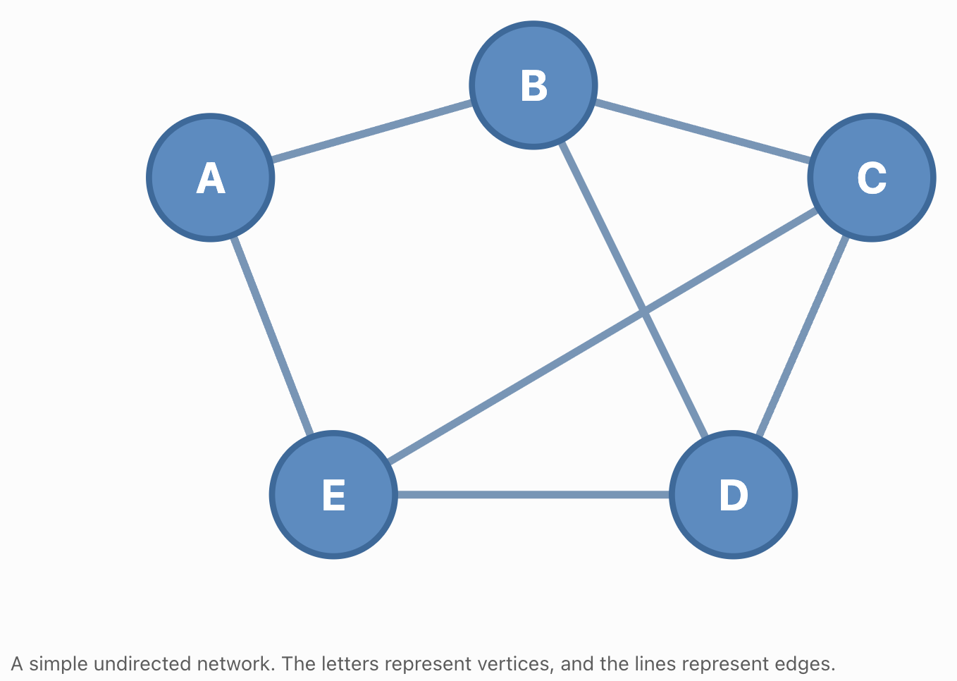
Interpreting the Network
Each vertex may represent a computer.
Each edge may represent a communication connection.
A path between two vertices represents a possible route for information to travel.
Counting Edges in a Complete Network
A complete graph is a graph in which every pair of distinct vertices is connected by an edge.
Suppose a network contains n computers.
Every computer is directly connected to every other computer.
How many connections are required?
The number of edges is:
E = n(n − 1)/2
Why Divide by Two?
Each connection joins two computers.
Counting connections from each computer counts every edge twice.
Therefore, we divide by 2.
Worked Example
A complete network contains six computers.
E = 6(6 − 1)/2
= 6 × 5/2
E = 15
Fifteen connections are required.
Connection to Combinations
Each edge corresponds to choosing two distinct vertices.
Therefore:
E = C(n,2)
This demonstrates how graph theory and combinatorics are connected.
Directed and Undirected Networks
Undirected Networks
An undirected edge represents a connection that works in both directions.
For example:
A — B
may represent a two-way communication link.
Directed Networks
A directed edge represents a connection with a specified direction.
For example:
A → B
indicates a connection from A to B.
Directed networks are useful for representing:
-
One-way roads.
-
Webpage links.
-
Information flow.
-
Dependencies between tasks.
-
Certain communication systems.
Counting Possible Directed Connections
For n vertices, if every ordered pair of distinct vertices can be connected:
Maximum directed edges = n(n − 1)
For five vertices:
5 × 4 = 20
This assumes no self-loops and at most one directed edge for each ordered pair.
Paths Through Networks
A path is a sequence of connected vertices.
Paths are important because information must travel through networks.
Example
Suppose a message can travel from A to D using:
A → B → D
or:
A → C → D
There are two possible routes.
If an additional route exists:
A → B → C → D
there are three routes.
Counting Paths
The number of possible paths depends on the network structure.
In some problems, the multiplication principle can be used.
Worked Example
A communication system has:
-
3 possible first-stage routes.
-
4 possible second-stage routes.
-
2 possible third-stage routes.
If every combination of choices produces a distinct valid route:
Total routes = 3 × 4 × 2
= 24
There are 24 possible routes.
Shortest-Path Problems
Many network problems involve finding the shortest or least expensive route between two vertices.
Edges may have weights representing:
-
Distance.
-
Time.
-
Cost.
-
Energy consumption.
-
Communication delay.
A weighted graph is a graph in which edges have numerical values.
Example
Suppose the network has the following connections:
|
Connection |
Distance |
|---|---|
|
A–B |
4 km |
|
A–C |
7 km |
|
B–C |
2 km |
|
B–D |
6 km |
|
C–D |
3 km |
Find the shortest route from A to D.
Possible routes include:
A → B → D
Distance = 4 + 6 = 10 km
A → C → D
Distance = 7 + 3 = 10 km
A → B → C → D
Distance = 4 + 2 + 3 = 9 km
Shortest route = A → B → C → D
Total distance = 9 km
For larger networks, algorithms such as Dijkstra's algorithm can find shortest paths efficiently when edge weights are non-negative.

Probability in Computer Networks
Computer networks experience uncertain events such as:
-
Transmission errors.
-
Equipment failures.
-
Packet loss.
-
Communication delays.
-
Temporary connection interruptions.
Probability helps engineers estimate the reliability of these systems.
Example: Independent Connection Failures
Suppose a network connection has a 2% probability of failing during a particular period.
Then:
P(connection works) = 0.98
If three independent connections must all work for communication to succeed:
P(all work) = 0.98³
≈ 0.9412
There is approximately a 94.12% probability that all three connections work.
The probability of at least one failure is:
P(at least one fails) = 1 − 0.98³
≈ 0.0588
There is approximately a 5.88% probability of at least one connection failure.
Network Redundancy
Redundancy means providing additional components or pathways so that a system can continue functioning if one part fails.
Suppose two independent network links connect the same devices.
Each link has a 10% probability of failing.
Communication fails only if both links fail.
Probability Both Links Fail
P(both fail) = 0.10 × 0.10
= 0.01
Probability Communication Remains Available
P(at least one works) = 1 − 0.01
= 0.99
The network has a 99% probability of remaining connected during the specified period.
Interpretation
Redundant connections can improve reliability.
However, the independence assumption is important.
If both links can fail because of the same power outage or physical damage, the actual reliability may be lower.

Reliability of Series and Parallel Networks
Two common reliability structures are series systems and parallel systems.
Series System
In a series system, every component must work.
If component reliabilities are independent:
R_series = R₁ × R₂ × ... × Rₙ
Example
Three components have reliabilities:
0.95, 0.90, and 0.98
Overall reliability:
R = 0.95 × 0.90 × 0.98
R = 0.8379
The system has an 83.79% probability of functioning.
Parallel System
In a parallel system, at least one component must work.
If failures are independent:
R_parallel = 1 − (1 − R₁)(1 − R₂)...(1 − Rₙ)
Example
Two independent components each have reliability 0.90.
R = 1 − (0.10 × 0.10)
R = 0.99
The system has a 99% probability of functioning.
This shows how probability and network structure can be combined to improve system design.
Probability and Randomized Algorithms
Some computer algorithms use random choices as part of their operation.
These are called randomized algorithms.
Randomness may help an algorithm:
-
Select samples.
-
Explore possible solutions.
-
Avoid predictable behaviour.
-
Estimate numerical quantities.
-
Distribute workloads.
Example: Random Sampling
Suppose a computer must estimate the average value of a very large dataset.
Instead of processing every value, it may randomly select a sample.
The sample mean can provide an estimate of the population mean.
Larger representative samples generally produce more stable estimates.
Monte Carlo Algorithms
Monte Carlo algorithms use random sampling to estimate quantities or solve problems approximately.
For example, random points can be used to estimate the value of π.
Las Vegas Algorithms
Las Vegas algorithms use randomness but, when they return a result, that result is correct.
Their running time may vary.
This differs from Monte Carlo algorithms, which may return an approximate or occasionally incorrect result depending on the algorithm.
Counting Possible Network Configurations
Combinatorics can also be used to count possible network structures.
Suppose a simple undirected network contains four labelled vertices.
There are:
C(4,2) = 6
possible edges.
Each edge can either:
-
Be present.
-
Be absent.
Therefore, the total number of possible simple undirected graphs is:
2⁶ = 64
General Formula
For n labelled vertices, the number of possible edges is:
C(n,2) = n(n − 1)/2
Therefore:
Number of possible simple undirected graphs = 2^[n(n − 1)/2]
This assumes no self-loops and at most one edge between any pair of vertices.
Example
For five labelled vertices:
Possible edges:
5 × 4/2 = 10
Possible graphs:
2¹⁰
= 1,024
The number of possible network structures increases rapidly as the number of vertices increases.
Practical Application: Secure Communication
When someone sends information over the internet, several mathematical systems work together.
Coding Theory
Error-detecting and error-correcting codes help identify or repair corrupted information.
Cryptography
Encryption protects the confidentiality of transmitted information.
Authentication and integrity mechanisms help detect unauthorized modification or impersonation.
Network Theory
Routing algorithms determine how information travels between devices.
Probability
Probability models estimate transmission errors, connection failures, and system reliability.
Combinatorics
Counting principles help determine codeword possibilities, key spaces, and network configurations.
These mathematical ideas work together to support reliable and secure digital communication.
Practical Application: QR Codes
QR codes store information using patterns of dark and light modules.
The information is represented digitally.
Error-correction techniques allow many QR codes to remain readable even when some parts are damaged or obscured.
QR codes use Reed–Solomon error correction, a more advanced coding method based on finite-field mathematics.
Combinatorics and algebra help explain how additional information can be used to detect and correct errors.

Practical Application: Data Storage
Digital storage devices must preserve information despite possible errors.
Errors may arise from:
-
Electrical interference.
-
Physical damage.
-
Ageing components.
-
Manufacturing defects.
-
Read and write failures.
Error-correcting codes add redundancy so that certain errors can be detected or corrected.
The design of these systems involves balancing:
-
Storage capacity.
-
Reliability.
-
Processing speed.
-
Error-correction capability.
More redundancy can improve reliability, but it also requires additional storage space.
Evaluating Mathematical Models
Mathematical models used in networks, coding, and cryptography depend on assumptions.
Important Questions
Are errors independent?
Transmission errors may occur in bursts rather than independently.
Are all outcomes equally likely?
Passwords and network failures may have highly unequal probabilities.
Are all connections equally reliable?
Some network links may be more vulnerable than others.
Does the model include shared failures?
Several components may fail because of a single event.
Are the mathematical methods appropriate?
A simple model may not capture all the details of a real system.
Is the security model realistic?
A large key space is not sufficient if the encryption algorithm or implementation is vulnerable.
Evaluating these assumptions is essential for interpreting mathematical results correctly.
Common Mistakes
Confusing permutations and combinations
Permutations consider order, while combinations do not.
Forgetting that repetition may be allowed
Password calculations depend on whether characters can repeat.
Assuming all passwords are equally likely
Human-generated passwords are often predictable.
Believing a large key space guarantees security
Security also depends on algorithms, implementations, and key management.
Confusing error detection with error correction
Detecting an error does not necessarily identify how to repair it.
Assuming parity bits detect every error
A single parity bit cannot detect every possible pattern of bit flips.
Calculating Hamming distance incorrectly
Only positions containing different symbols should be counted.
Assuming network failures are independent
Shared causes can produce simultaneous failures.
Confusing series and parallel reliability
Series systems require every component to work, while parallel systems require at least one functioning component.
Double-counting network edges
In an undirected network, each connection should be counted only once.
Assuming the shortest path is always the fastest
Distance, travel time, and communication delay may be different edge weights.
Ignoring the assumptions of probability models
A mathematically correct calculation can produce an unrealistic prediction if the assumptions are inappropriate.
Key Terms
-
Combinatorics: The mathematical study of counting, arranging, and selecting objects.
-
Addition Principle: A counting rule for mutually exclusive alternatives.
-
Multiplication Principle: A counting rule for processes involving successive choices.
-
Permutation: An arrangement in which order matters.
-
Combination: A selection in which order does not matter.
-
Binary Digit (Bit): A digit with value 0 or 1.
-
Binary String: A sequence of binary digits.
-
Coding Theory: The mathematical study of representing information for efficient and reliable storage or transmission.
-
Codeword: A valid encoded sequence of symbols.
-
Error Detection: Identifying whether transmitted or stored information has been corrupted.
-
Error Correction: Recovering the original information from certain corrupted messages.
-
Parity Bit: An additional bit used to check the parity of a binary message.
-
Even Parity: A coding rule requiring an even total number of 1s.
-
Repetition Code: An error-correcting code that repeats information symbols.
-
Code Rate: The ratio of original information symbols to total transmitted symbols.
-
Hamming Distance: The number of positions in which two equal-length strings differ.
-
Minimum Distance: The smallest Hamming distance between distinct valid codewords.
-
Bit Error Rate: The proportion or probability of transmitted bits that are received incorrectly.
-
Cryptography: The study of techniques for protecting information.
-
Encryption: Transforming readable information into ciphertext.
-
Decryption: Recovering plaintext from ciphertext.
-
Plaintext: Information before encryption.
-
Ciphertext: Encrypted information.
-
Encryption Key: Information used by an encryption algorithm.
-
Key Space: The set of all possible encryption keys.
-
Substitution Cipher: A cipher that replaces symbols according to a substitution rule.
-
Caesar Cipher: A substitution cipher based on shifting letters through the alphabet.
-
Modular Arithmetic: Arithmetic involving remainders after division by a fixed number.
-
Frequency Analysis: A method of analysing symbol frequencies to investigate encrypted messages.
-
Network: A collection of objects connected by relationships.
-
Graph: A mathematical structure consisting of vertices and edges.
-
Vertex: A node representing an object in a network.
-
Edge: A connection between two vertices.
-
Directed Graph: A graph whose edges have directions.
-
Undirected Graph: A graph whose edges have no direction.
-
Weighted Graph: A graph whose edges have numerical values.
-
Complete Graph: A graph in which every pair of distinct vertices is connected.
-
Path: A sequence of connected vertices.
-
Shortest Path: A route between vertices with the smallest total weight.
-
Network Reliability: The probability that a network performs its required function.
-
Redundancy: Additional components or connections included to improve reliability.
-
Series System: A system that works only when every required component works.
-
Parallel System: A system that works when at least one of several alternative components works.
-
Randomized Algorithm: An algorithm that uses random choices during execution.
-
Monte Carlo Algorithm: A randomized algorithm that produces estimates or results with a specified probability of error.
-
Las Vegas Algorithm: A randomized algorithm that always returns a correct result when it terminates, although its running time may vary.
Key Takeaways
-
Combinatorics plays an important role in coding theory, cryptography, and computer networks.
-
The multiplication principle can be used to count binary strings, passwords, and possible routes.
-
A binary string of length n has 2ⁿ possible values.
-
Combinations can count binary strings containing a specified number of ones.
-
Coding theory develops methods for detecting and correcting errors in digital information.
-
Parity bits can detect odd numbers of bit flips but cannot detect every possible error pattern.
-
Repetition codes use redundancy to correct certain errors.
-
Hamming distance measures the number of differing positions between equal-length strings.
-
A code's minimum Hamming distance determines its guaranteed error-detection and correction capabilities.
-
Binomial probability can model independent bit errors.
-
Cryptography uses mathematical methods to protect digital information.
-
Password and encryption key spaces can be counted using combinatorial principles.
-
Longer passwords and larger key spaces generally increase the number of possibilities an attacker must consider.
-
A large key space alone does not guarantee cryptographic security.
-
Networks can be represented using graphs consisting of vertices and edges.
-
A complete undirected graph with n vertices has n(n − 1)/2 edges.
-
Weighted graphs can model distances, costs, and communication delays.
-
Shortest-path algorithms help identify efficient routes through networks.
-
Probability can estimate the reliability of network components and communication links.
-
Redundancy can improve network reliability by providing alternative paths or components.
-
Randomized algorithms use probability to solve or approximate computational problems.
-
Coding theory, cryptography, network theory, and probability work together in modern communication systems.
Check Your Understanding
Recall and Understanding
-
Explain how combinatorics is used in coding theory and cryptography.
-
Define a bit and a binary string.
-
Explain the purpose of parity bits in error detection.
-
Define Hamming distance and explain why it is useful.
-
Describe the difference between a directed graph and an undirected graph.
Application
-
How many different binary strings of length 10 are possible?
-
How many eight-bit binary strings contain exactly four ones?
-
A password contains seven characters, each selected from 26 lowercase letters and 10 digits. If repetition is allowed, how many passwords are possible?
-
Calculate the Hamming distance between 10110110 and 10011100.
-
A complete undirected network contains eight computers. How many direct connections are required?
Analysis and Challenge
-
A 12-bit message is transmitted, and each bit has an independent 2% probability of error. Calculate the probability that exactly two bits are corrupted.
-
A communication system uses three independent links in series, each with 95% reliability. Calculate the overall reliability. Then determine the reliability if the three links instead form a parallel system where any one functioning link is sufficient.
-
A substitution cipher uses a permutation of the 26-letter English alphabet. Explain why the large number of possible substitutions does not guarantee strong encryption.
-
A network contains five labelled vertices. Calculate the number of possible simple undirected graphs. Explain the counting principle used.
-
Design a small network containing at least five vertices and seven edges. Assign weights to the edges, identify the shortest path between two selected vertices, and explain how the network could be made more reliable.
Final Summary
Networks, coding theory, and cryptography demonstrate how combinatorics and probability are applied in modern computer science.
Combinatorics provides methods for counting possible messages, passwords, encryption keys, error patterns, and network configurations.
Coding theory uses mathematical redundancy to detect and correct errors in digital communication.
Cryptography uses counting principles, modular arithmetic, and other mathematical structures to protect information.
Graph theory provides a framework for representing networks and analysing connections, paths, and routes.
Probability helps estimate transmission errors, component failures, and overall network reliability.
Together, these mathematical ideas support secure communication, reliable data storage, efficient routing, and modern digital technology.
The central principle is that counting possible outcomes, analysing probabilities, and understanding mathematical structures allow us to design more reliable and secure information systems.
4. Probability in Science and Engineering
Learning outcomes
- I can apply probability models in science.
- I can analyse reliability problems.
- I can model engineering systems.
- I can interpret probabilistic data.
- I can solve authentic STEM applications.
Probability in Science and Engineering
Introduction to Probability in Science and Engineering
Science and engineering involve measurements, predictions, experiments, and decisions that are rarely completely certain.
Scientists investigate natural processes that contain randomness or measurement uncertainty. Engineers design systems that must operate reliably despite variations in materials, environmental conditions, and component performance.
Probability provides mathematical tools for understanding these uncertainties.
For example:
-
What is the probability that a machine operates without failure for five years?
-
How likely is a measurement to fall within an acceptable range?
-
What is the probability that a manufactured component is defective?
-
How reliable is an electrical system containing several components?
-
How many radioactive atoms are expected to decay during a given period?
-
What is the probability that a bridge experiences a load exceeding its design threshold?
These problems can be investigated using probability distributions, reliability models, statistical reasoning, and simulation.
Probability in science and engineering helps us quantify uncertainty, evaluate risks, and make informed decisions about real systems.


Why Probability Is Important in STEM
Many scientific and engineering processes contain uncertainty because of:
-
Natural randomness.
-
Measurement limitations.
-
Variations in manufacturing.
-
Environmental changes.
-
Material imperfections.
-
Human factors.
-
Equipment failures.
-
Incomplete information.
Probability allows these uncertainties to be represented mathematically.
Deterministic and Probabilistic Models
A deterministic model produces the same result whenever the same inputs are used.
For example:
Distance = Speed × Time
If speed and time are known exactly, the calculated distance is fixed.
A probabilistic model allows uncertain inputs or outcomes.
For example, the time until a machine fails may be represented by a probability distribution rather than a single fixed value.
Comparison
|
Feature |
Deterministic model |
Probabilistic model |
|---|---|---|
|
Inputs |
Fixed |
May be uncertain |
|
Output |
Single predicted value |
Range or distribution of outcomes |
|
Randomness |
Not explicitly included |
Explicitly represented |
|
Example |
Ideal motion calculation |
Equipment failure prediction |
|
Main purpose |
Predict a specific outcome |
Quantify uncertainty and risk |
Both types of models are important in science and engineering.
Random Variables in Scientific Models
A random variable assigns a numerical value to the outcome of a random process.
Random variables can be discrete or continuous.
Discrete Random Variables
A discrete random variable takes values from a finite or countably infinite set.
Examples include:
-
Number of defective components.
-
Number of radioactive decays.
-
Number of equipment failures.
-
Number of particles detected.
-
Number of vehicles arriving.
Continuous Random Variables
A continuous random variable can take any real value within an interval or collection of intervals.
Examples include:
-
Temperature.
-
Pressure.
-
Mass.
-
Length.
-
Voltage.
-
Time until failure.
-
Measurement error.
The type of random variable helps determine which probability model is appropriate.
Choosing a Probability Distribution
Different scientific problems require different probability distributions.
|
Distribution |
Type |
Common STEM application |
|---|---|---|
|
Bernoulli |
Discrete |
Whether a component passes inspection |
|
Binomial |
Discrete |
Number of defective items in a sample |
|
Poisson |
Discrete |
Number of events in a time interval |
|
Geometric |
Discrete |
Trials until the first success |
|
Normal |
Continuous |
Measurement variation and manufacturing dimensions |
|
Exponential |
Continuous |
Time between events or failures under a constant-rate model |
|
Uniform |
Continuous |
Values equally likely across an interval |
A probability distribution should be selected according to the characteristics of the system, not simply because a familiar formula is available.
Binomial Models in Quality Control
Manufacturing systems produce large numbers of components.
Some components may fail to meet quality standards.
Suppose each component has a probability p of being defective.
If n components are selected independently and the defect probability remains constant, the number of defective components follows a binomial distribution.
X ~ B(n,p)
The probability of exactly k defective components is:
P(X = k) = C(n,k) × pᵏ × (1 − p)^(n−k)
Worked Example: Defective Components
A factory produces electronic components.
Each component has a 4% probability of being defective.
Ten components are selected independently.
Find the probability that exactly two are defective.
Given:
n = 10
p = 0.04
k = 2
Substitute:
P(X = 2) = C(10,2) × 0.04² × 0.96⁸
Since:
C(10,2) = 45
P(X = 2) = 45 × 0.0016 × 0.96⁸
P(X = 2) ≈ 0.0519
There is approximately a 5.19% probability that exactly two of the ten components are defective.
Model Assumptions
The calculation assumes:
-
Each component is classified as defective or non-defective.
-
The defect probability remains 0.04.
-
The selected components are independent.
-
The number of components is fixed.
If defects occur in clusters because of a faulty machine, independence may be unrealistic.

Probability of At Least One Defect
In engineering, it is often useful to calculate the probability that at least one component fails.
The complement rule simplifies this calculation.
P(at least one defect) = 1 − P(no defects)
For n independent components, each with defect probability p:
P(at least one defect) = 1 − (1 − p)ⁿ
Worked Example
Suppose each component has a 2% probability of being defective.
A sample contains 20 components.
P(at least one defect) = 1 − 0.98²⁰
≈ 1 − 0.6676
P(at least one defect) ≈ 0.3324
There is approximately a 33.24% probability that at least one component is defective.
Interpretation
Even a relatively small individual defect probability can produce a substantial probability of at least one defect when many components are involved.
Poisson Models in Science
The Poisson distribution models the number of events occurring within a fixed interval when events follow an appropriate constant-rate process.
Examples include:
-
Radioactive decay counts.
-
Particle detections.
-
Equipment faults.
-
Calls arriving at a control centre.
-
Certain types of material defects.
If the average number of events is λ:
P(X = k) = e^(−λ) × λᵏ/k!
where:
-
λ is the expected number of events in the interval.
-
k is the number of events.
-
e ≈ 2.71828.
Worked Example: Radioactive Decay
A detector records an average of three radioactive decay events per minute.
Assume the counts follow a Poisson distribution.
Find the probability of recording exactly five events in one minute.
Given:
λ = 3
k = 5
P(X = 5) = e^(−3) × 3⁵/5!
= e^(−3) × 243/120
P(X = 5) ≈ 0.1008
There is approximately a 10.08% probability of recording exactly five events in one minute.

Expected Value and Variance in Scientific Data
The expected value describes the probability-weighted average of a random variable.
For a discrete random variable:
E(X) = Σ[x × P(X = x)]
The variance measures the spread of possible outcomes around the mean.
Var(X) = E[(X − μ)²]
The standard deviation is:
σ = √Var(X)
Important Distribution Properties
For a binomial random variable:
E(X) = np
Var(X) = np(1 − p)
For a Poisson random variable:
E(X) = λ
Var(X) = λ
Example
Suppose:
X ~ B(100, 0.03)
Expected defects:
E(X) = 100 × 0.03
E(X) = 3
Variance:
Var(X) = 100 × 0.03 × 0.97
Var(X) = 2.91
Standard deviation:
σ = √2.91
σ ≈ 1.71
The expected number of defective components is three, with a standard deviation of approximately 1.71 components.
The Normal Distribution in Engineering
Many continuous measurements are approximately normally distributed.
Examples include:
-
Manufactured component lengths.
-
Measurement errors.
-
Certain material properties.
-
Repeated laboratory measurements.
The normal distribution is symmetrical and bell-shaped.
It is described by:
-
Mean μ.
-
Standard deviation σ.

Standardizing Measurements
A value x from a normal distribution can be converted into a z-score.
z = (x − μ)/σ
The z-score measures how many standard deviations a value lies above or below the mean.
Worked Example: Manufacturing Dimensions
A factory manufactures metal rods.
Their lengths are approximately normally distributed with:
Mean = 100 mm
Standard deviation = 2 mm
Find the probability that a rod is shorter than 97 mm.
Step 1: Calculate the z-Score
z = (97 − 100)/2
z = −1.5
Step 2: Use the Standard Normal Distribution
P(Z < −1.5) ≈ 0.0668
Interpretation
Approximately 6.68% of rods are expected to be shorter than 97 mm under the model.
This information can help engineers evaluate manufacturing tolerances.
Engineering Tolerances
A tolerance is the permitted variation in a manufactured measurement.
Suppose a component must have a diameter between 19.5 mm and 20.5 mm.
The manufacturing process produces diameters that are normally distributed with:
μ = 20.0 mm
σ = 0.2 mm
Find the probability that a component meets the specification.
Step 1: Calculate the Lower z-Score
z₁ = (19.5 − 20.0)/0.2
z₁ = −2.5
Step 2: Calculate the Upper z-Score
z₂ = (20.5 − 20.0)/0.2
z₂ = 2.5
Step 3: Find the Probability
P(−2.5 ≤ Z ≤ 2.5)
≈ 0.9876
P(within tolerance) ≈ 98.76%
Interpretation
Approximately 98.76% of components are expected to meet the specification.
The remaining 1.24% are expected to fall outside the permitted range.

Reliability Engineering
Reliability engineering investigates the probability that a system performs its required function for a specified period under specified conditions.
Reliability is important in:
-
Aircraft.
-
Vehicles.
-
Power systems.
-
Medical equipment.
-
Computer networks.
-
Manufacturing machinery.
-
Communication systems.
The reliability of a component over time t is:
R(t) = P(T > t)
where:
T = time until failure.
Interpretation
If:
R(1000) = 0.95
then the component has a 95% probability of operating for more than 1,000 time units under the stated conditions.
The time units might be hours, days, or years.
Series Systems
In a series system, every required component must work for the system to function.
For independent components:
R_system = R₁ × R₂ × ... × Rₙ
Worked Example
An engineering system contains three components.
Their reliabilities are:
R₁ = 0.98
R₂ = 0.95
R₃ = 0.99
The system works only if all three components work.
Calculate:
R_system = 0.98 × 0.95 × 0.99
R_system ≈ 0.9217
The probability that the complete system operates successfully is approximately 92.17%.
Important Principle
Adding more required components to a series system generally reduces overall reliability when each additional component has reliability below 1.
Parallel Systems
In a parallel system, the system continues functioning if at least one of several alternative components works.
For independent components:
R_system = 1 − (1 − R₁)(1 − R₂)...(1 − Rₙ)
Worked Example
A system contains two independent backup pumps.
Each pump has reliability:
R = 0.90
The system works if at least one pump operates.
Probability both pumps fail:
0.10 × 0.10 = 0.01
Therefore:
R_system = 1 − 0.01
R_system = 0.99
The system has a 99% probability of operating successfully.
Why Redundancy Helps
Adding independent backup components can improve reliability.
However, common failures such as power outages, flooding, or overheating may affect several components simultaneously.

Interactive Reliability Comparison
Explore how component reliability and the number of components affect series and parallel systems.
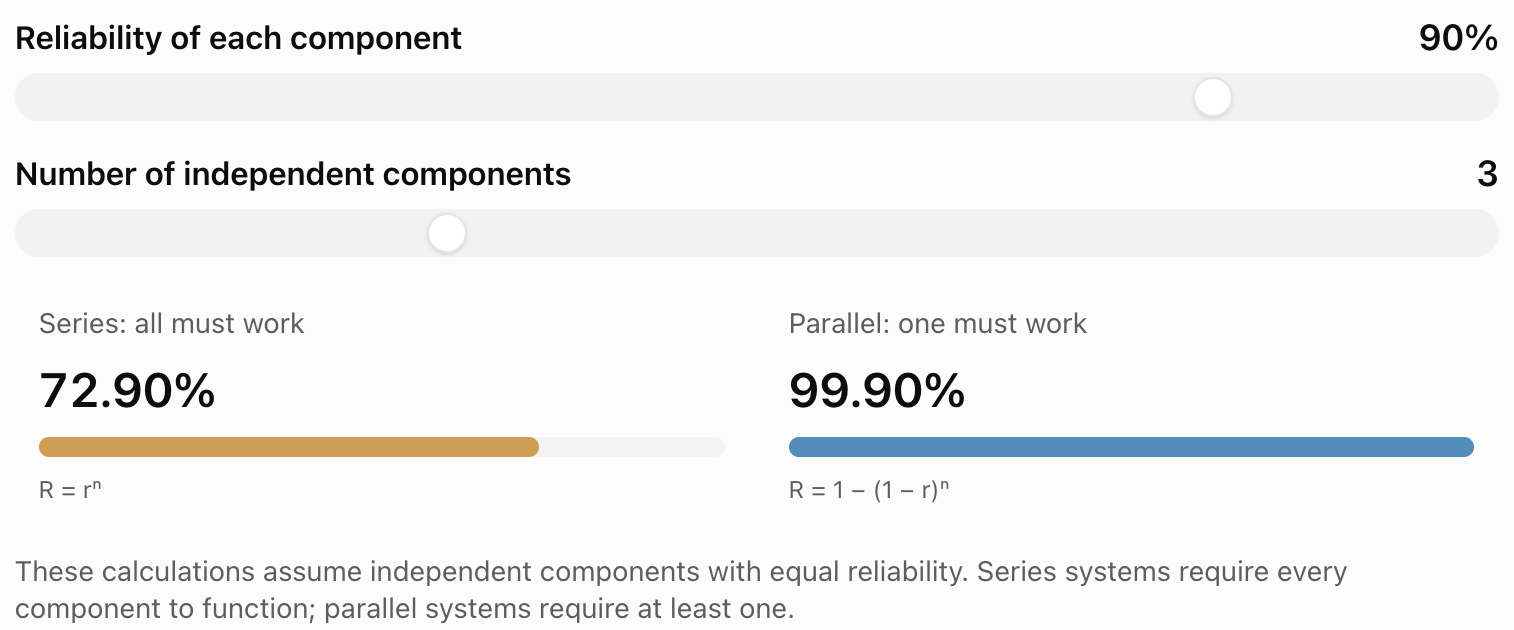
Exponential Reliability Models
Some engineering components are modelled using an exponential distribution for time until failure.
This model assumes a constant failure rate.
The reliability function is:
R(t) = e^(−λt)
where:
-
R(t) is the probability of surviving beyond time t.
-
λ is the constant failure rate.
-
t is elapsed time.
Worked Example
A component has a constant failure rate of:
λ = 0.002 failures per hour
Find the probability that it operates for at least 100 hours.
R(100) = e^(−0.002 × 100)
= e^(−0.2)
R(100) ≈ 0.8187
There is approximately an 81.87% probability that the component survives beyond 100 hours.
Mean Time to Failure
For an exponential model:
MTTF = 1/λ
For this component:
MTTF = 1/0.002
MTTF = 500 hours
This is the expected time to failure under the model.
Limitations
A constant failure rate may not be realistic for components that wear out with age.
Other models, such as the Weibull distribution, may be more appropriate for systems with changing failure rates.
Probability in Structural Engineering
Structural engineers must consider uncertain loads and material properties.
Examples include:
-
Wind forces.
-
Vehicle loads.
-
Earthquake forces.
-
Material strength.
-
Construction variations.
A structure is at risk when the applied load exceeds its resistance.
Let:
L = applied load
S = structural strength
Failure occurs when:
L > S
Therefore:
P(failure) = P(L > S)
Simplified Example
Suppose a component can withstand a maximum load of 500 N.
The applied load is normally distributed with:
μ = 400 N
σ = 50 N
Find the probability that the load exceeds 500 N.
Calculate the z-score:
z = (500 − 400)/50
z = 2
From the standard normal distribution:
P(Z > 2) ≈ 0.0228
P(failure) ≈ 2.28%
Interpretation
Under this simplified model, approximately 2.28% of loading events exceed the threshold.
Real structural reliability analysis is more complicated because both load and resistance may vary, and loads may be correlated or change over time.

Probability in Experimental Science
Scientific measurements contain uncertainty.
Repeated measurements of the same quantity may produce slightly different results because of:
-
Instrument resolution.
-
Environmental variation.
-
Random noise.
-
Observer differences.
-
Experimental conditions.
Probability distributions help describe this variation.
Example: Repeated Measurements
A student measures the length of an object five times.
The results are:
12.1 cm, 12.3 cm, 12.2 cm, 12.0 cm, 12.4 cm
Mean:
x̄ = (12.1 + 12.3 + 12.2 + 12.0 + 12.4)/5
x̄ = 12.2 cm
The measurements vary around the mean.
A standard deviation can be calculated to describe the spread.
Important Distinction
Random measurement variation can often be reduced by taking repeated measurements and averaging.
Systematic errors, such as an incorrectly calibrated instrument, are not necessarily reduced by repetition.
Confidence Intervals in Engineering
A confidence interval estimates an unknown population parameter using sample data.
For a population mean with known population standard deviation σ, a 95% confidence interval is:
x̄ ± 1.96 × σ/√n
where:
-
x̄ is the sample mean.
-
σ is the population standard deviation.
-
n is the sample size.
Worked Example
A factory measures the diameter of 100 components.
The sample mean is:
x̄ = 20.1 mm
The known population standard deviation is:
σ = 0.5 mm
Calculate the standard error:
SE = 0.5/√100
= 0.05 mm
Margin of error:
1.96 × 0.05 = 0.098 mm
Confidence interval:
20.1 ± 0.098
20.002 mm to 20.198 mm
Interpretation
Using this method, approximately 95% of confidence intervals constructed from repeated samples would contain the true population mean, assuming the method's conditions are satisfied.
The interval estimates the mean diameter, not the range containing 95% of individual component diameters.
Monte Carlo Simulation in Engineering
Monte Carlo simulation uses repeated random sampling to investigate uncertain systems.
It is particularly useful when several variables are uncertain.
Example: Manufacturing Dimensions
Suppose the length and width of a manufactured plate vary slightly.
The area is:
A = L × W
If both L and W are uncertain, the area is also uncertain.
A Monte Carlo simulation can:
-
Generate a random length from an appropriate distribution.
-
Generate a random width.
-
Calculate the area.
-
Repeat thousands of times.
-
Analyse the distribution of calculated areas.
The simulation can estimate:
-
Mean area.
-
Standard deviation of area.
-
Probability that area exceeds a limit.
-
Probability that area falls within specifications.

Practical Application: Battery Reliability
Suppose a battery-powered system requires two independent batteries connected in parallel.
Each battery has a 95% probability of functioning throughout a mission.
The system works if at least one battery functions.
Probability both batteries fail:
0.05 × 0.05 = 0.0025
System reliability:
R = 1 − 0.0025
R = 0.9975
The system has a 99.75% probability of remaining operational.
Engineering Interpretation
Redundancy improves reliability.
However, if both batteries depend on the same charging system or are exposed to the same extreme temperature, failures may be correlated.
The independence assumption must be evaluated.
Practical Application: Medical Testing
Probability models are important in medical diagnostics.
A test may have:
-
Sensitivity: Probability of a positive result when the condition is present.
-
Specificity: Probability of a negative result when the condition is absent.
The probability that a person actually has a condition after testing positive also depends on how common the condition is.
Worked Example
Suppose:
-
1% of a population has a particular condition.
-
The test has 95% sensitivity.
-
The test has 90% specificity.
We want:
P(condition | positive)
Using Bayes' theorem:
P(condition | positive) = P(positive | condition)P(condition) / P(positive)
Calculate:
P(positive) = 0.95 × 0.01 + 0.10 × 0.99
= 0.0095 + 0.099
= 0.1085
Therefore:
P(condition | positive) = 0.0095/0.1085
≈ 0.0876
Approximately 8.76% of positive test results correspond to people who have the condition under these assumptions.
Interpretation
Even a test with relatively high sensitivity can produce many false positives when the condition is uncommon.
This demonstrates why base rates are important in scientific probability.
Practical Application: Environmental Monitoring
Environmental scientists use probability to investigate uncertain natural processes.
Examples include:
-
Rainfall.
-
Flooding.
-
Wind speed.
-
Pollution levels.
-
Temperature extremes.
-
Wildfire occurrence.
Example: Extreme Rainfall
Suppose a simplified model estimates a 5% probability of rainfall exceeding a particular threshold in any given year.
Assume annual exceedance events are independent and the probability remains constant.
The probability of no exceedance over ten years is:
P(no exceedance) = 0.95¹⁰
≈ 0.5987
Therefore:
P(at least one exceedance) = 1 − 0.95¹⁰
≈ 0.4013
There is approximately a 40.13% probability of at least one exceedance during ten years.
Interpretation
A relatively small annual probability can correspond to a much larger probability over a longer period.
This is important when designing infrastructure to withstand rare environmental events.

Interpreting Probabilistic Data
Scientific and engineering results often include probabilities, confidence intervals, and uncertainty estimates.
These values must be interpreted carefully.
Example
An engineer reports:
"The probability of system failure during one year is 0.002."
This means:
P(failure) = 0.002
As a percentage:
0.002 × 100% = 0.2%
The probability of successful operation during the year is:
1 − 0.002 = 0.998
= 99.8%
Important Questions
When interpreting probabilistic data, ask:
-
What event is being measured?
-
What time period is involved?
-
What assumptions were made?
-
How were the probabilities estimated?
-
Are the events independent?
-
Is the sample size sufficient?
-
How uncertain are the estimates?
-
What are the consequences if the event occurs?
A probability should not be interpreted without its context.
Comparing Engineering Designs
Suppose two engineering designs are available.
Design A
-
Cost: $50,000.
-
Probability of failure during the first year: 0.04.
-
Financial consequence of failure: $100,000.
Expected failure cost:
0.04 × $100,000
= $4,000
Expected total cost:
$50,000 + $4,000
= $54,000
Design B
-
Cost: $55,000.
-
Probability of failure during the first year: 0.01.
-
Financial consequence of failure: $100,000.
Expected failure cost:
0.01 × $100,000
= $1,000
Expected total cost:
$55,000 + $1,000
= $56,000
Comparison
|
Measure |
Design A |
Design B |
|---|---|---|
|
Initial cost |
$50,000 |
$55,000 |
|
Failure probability |
4% |
1% |
|
Expected failure cost |
$4,000 |
$1,000 |
|
Expected total cost |
$54,000 |
$56,000 |
Design A has the lower expected financial cost.
Design B has the lower probability of failure.
Interpretation
If failure could endanger people or cause severe environmental harm, Design B may be preferable despite its higher expected monetary cost.
Engineering decisions must consider safety requirements and consequences, not just expected financial value.
Evaluating Probability Models
Probability models are only useful when their assumptions reasonably represent the system.
Independence
Do component failures occur independently?
Constant Probabilities
Do failure probabilities change with age, temperature, or operating conditions?
Distribution Choice
Does the selected distribution match the observed data?
Sample Quality
Are the observations representative?
Rare Events
Does the model account for uncommon but severe outcomes?
Model Validation
Do predictions agree with real observations?
Sensitivity Analysis
How do results change when uncertain parameters are adjusted?
These questions help determine whether a model is suitable for a scientific or engineering application.
Common Mistakes
Assuming all events are independent
Many engineering failures share common causes.
Using the wrong probability distribution
Counts, measurements, and waiting times may require different models.
Confusing reliability with failure probability
Reliability is the probability of successful operation, while failure probability is its complement over the same period.
Using series reliability formulas for parallel systems
The system structure determines the correct calculation.
Assuming a constant failure rate applies to every component
Some components become more likely to fail as they age.
Confusing expected value with a guaranteed outcome
Expected values describe averages, not certain results.
Misinterpreting confidence intervals
Confidence intervals estimate parameters and must be interpreted according to their construction.
Ignoring systematic measurement errors
Repeated measurements do not automatically remove calibration errors.
Assuming a low annual risk means a low long-term risk
Risk can accumulate over multiple years.
Ignoring the consequences of rare failures
Low-probability events may still be important when their consequences are severe.
Using precise calculations with unrealistic assumptions
Mathematical precision does not guarantee practical accuracy.
Key Terms
-
Probability Model: A mathematical representation of uncertain outcomes and their probabilities.
-
Random Variable: A numerical variable determined by the outcome of a random process.
-
Discrete Random Variable: A random variable with a finite or countably infinite set of values.
-
Continuous Random Variable: A random variable that can take any real value within an interval or collection of intervals.
-
Deterministic Model: A model producing a fixed result from specified inputs.
-
Probabilistic Model: A model incorporating uncertain inputs or outcomes.
-
Bernoulli Distribution: A probability model for one success-or-failure trial.
-
Binomial Distribution: A model for the number of successes in a fixed number of independent trials.
-
Poisson Distribution: A model for the number of events in an interval under appropriate constant-rate assumptions.
-
Normal Distribution: A symmetrical, bell-shaped continuous probability distribution.
-
Exponential Distribution: A continuous distribution often used for waiting times under a constant event rate.
-
Expected Value: The probability-weighted average of possible outcomes.
-
Variance: A measure of how widely outcomes are spread around the mean.
-
Standard Deviation: The square root of variance, measuring variability in the original units.
-
z-Score: The number of standard deviations a value lies above or below the mean.
-
Engineering Tolerance: The permitted variation in a manufactured measurement.
-
Quality Control: Processes used to assess whether products meet specified standards.
-
Defect Probability: The probability that a component fails to meet a required standard.
-
Reliability: The probability that a system performs its required function under specified conditions.
-
Failure Probability: The probability that a component or system fails during a specified period.
-
Series System: A system that requires all components to function.
-
Parallel System: A system that functions if at least one alternative component works.
-
Redundancy: Additional components or pathways included to improve reliability.
-
Failure Rate: A measure describing the frequency or instantaneous tendency of failures.
-
Mean Time to Failure (MTTF): The expected operating time before failure.
-
Measurement Uncertainty: Uncertainty associated with a measured quantity.
-
Sampling Error: Variation caused by estimating a population quantity using a sample.
-
Systematic Error: A consistent measurement error caused by bias or calibration problems.
-
Confidence Interval: A range calculated using a method designed to contain an unknown parameter at a specified long-run rate.
-
Monte Carlo Simulation: A method using repeated random sampling to estimate probabilities or numerical quantities.
-
Sensitivity Analysis: An investigation of how model results change when assumptions or parameters change.
-
Risk Assessment: The process of evaluating the probability and consequences of uncertain events.
-
Model Validation: Comparing model predictions with observations to assess suitability.
Key Takeaways
-
Probability models help scientists and engineers analyse uncertain processes and systems.
-
Scientific uncertainty may arise from natural randomness, measurement variation, or incomplete information.
-
Discrete models are useful for counts, while continuous models are useful for measurements and waiting times.
-
Binomial distributions can model the number of defective components under suitable assumptions.
-
Poisson distributions can model event counts in fixed intervals.
-
Normal distributions are useful for approximately symmetrical measurement variation.
-
Expected value describes the average outcome of a random variable.
-
Variance and standard deviation measure the spread of possible outcomes.
-
Reliability is the probability that a component or system performs successfully for a specified period.
-
Series systems require every component to work.
-
Parallel systems can continue operating when at least one alternative component works.
-
Redundancy can improve reliability when component failures are sufficiently independent.
-
Exponential reliability models assume a constant failure rate.
-
Manufacturing tolerances can be evaluated using probability distributions.
-
Confidence intervals provide estimates of unknown population parameters.
-
Monte Carlo simulations can investigate systems with several uncertain variables.
-
Bayes' theorem is useful for interpreting diagnostic tests and conditional probabilities.
-
Environmental risks may accumulate over time.
-
Engineering decisions must consider both the probability and consequences of failure.
-
Model assumptions should always be evaluated before interpreting results.
Check Your Understanding
Recall and Understanding
-
Explain why probability is important in science and engineering.
-
Distinguish between deterministic and probabilistic models.
-
Identify three probability distributions commonly used in STEM applications and give an example of each.
-
Define reliability and explain how it differs from failure probability.
-
Explain the difference between series and parallel engineering systems.
Application
-
A factory produces components with a 3% probability of being defective. Assuming independence, calculate the probability that exactly two of 15 components are defective.
-
A radiation detector records an average of four events per minute. Assuming a Poisson model, calculate the probability of recording exactly six events in one minute.
-
A machine component has a constant failure rate of 0.001 per hour. Calculate its reliability after 500 hours.
-
Three independent components in a series system have reliabilities of 0.95, 0.98, and 0.97. Calculate the system reliability.
-
Two independent backup systems each have reliability 0.92. Calculate the reliability of the parallel system.
Analysis and Challenge
-
A manufacturing process produces component lengths that are normally distributed with a mean of 50 mm and a standard deviation of 0.5 mm. Calculate the probability that a component is longer than 51 mm.
-
A structural component can withstand a maximum load of 800 N. Applied loads are normally distributed with a mean of 650 N and a standard deviation of 75 N. Estimate the probability that the load exceeds the component's capacity.
-
A factory is comparing two engineering designs. Design A costs $40,000 with a 5% probability of a $100,000 failure. Design B costs $45,000 with a 1% probability of the same failure. Calculate the expected total cost of each design and justify which may be preferable.
-
A flood has a 2% probability of exceeding a specified level in any given year. Assuming independence, calculate the probability of at least one exceedance during the next 25 years. Explain why this matters for infrastructure planning.
-
Design a probability model for a real-world STEM application. Identify the random variable, select an appropriate distribution, state the assumptions, perform a probability calculation, and explain how the results could inform a scientific or engineering decision.
Final Summary
Probability is an essential mathematical tool in science and engineering because real systems involve uncertainty.
Probability distributions help model random events, measurement variation, manufacturing defects, equipment failures, and environmental processes.
Reliability engineering uses probability to estimate whether components and systems will operate successfully under specified conditions.
Series and parallel reliability models demonstrate how system structure affects overall performance.
Statistical methods, including confidence intervals and Monte Carlo simulation, allow scientists and engineers to interpret uncertain data and investigate complex systems.
Probability also supports practical decisions involving quality control, safety, infrastructure, medical testing, and environmental risk.
The central principle is that probability does not eliminate uncertainty. Instead, it provides a mathematical framework for understanding uncertainty, estimating risk, and making better-informed scientific and engineering decisions.
5. Comprehensive Problem Solving
Learning outcomes
- I can solve complex multi-step probability and counting problems.
- I can combine multiple combinatorial techniques.
- I can select efficient solution strategies.
- I can justify mathematical reasoning.
- I can communicate complete mathematical solutions.
Comprehensive Problem Solving
Introduction to Comprehensive Problem Solving
Many probability and counting problems cannot be solved using a single formula. They require several mathematical ideas to be combined in a logical sequence.
For example:
-
How many passwords satisfy several restrictions?
-
What is the probability of drawing a particular combination of cards?
-
How many different committees can be formed when certain members must be included?
-
What is the probability that a manufactured system contains multiple defective components?
-
How many routes are possible through a network with restrictions?
-
How can we calculate probabilities when events are dependent?
These problems may involve permutations, combinations, conditional probability, probability distributions, complementary events, or several counting principles.
The most important skill is not memorizing more formulas. It is learning to recognize the structure of a problem, choose an efficient strategy, and communicate a complete mathematical solution.


A Systematic Approach to Complex Problems
Complex problems become more manageable when they are divided into smaller steps.
A useful problem-solving process is:
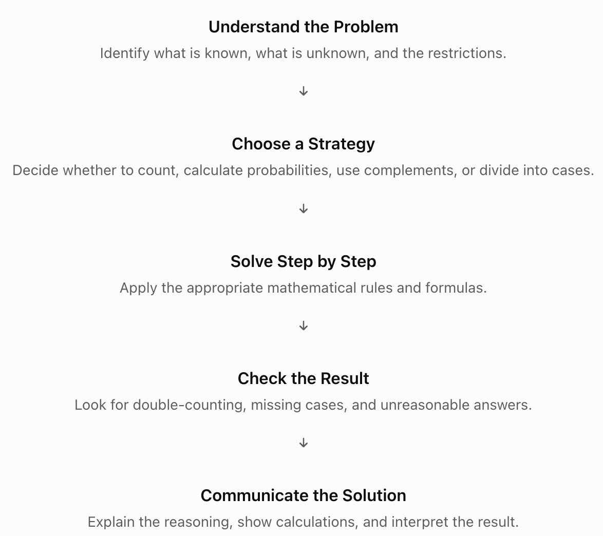
Recognizing the Structure of a Counting Problem
Before choosing a formula, ask several important questions.
Does Order Matter?
If order matters, permutations or arrangements may be appropriate.
If order does not matter, combinations may be appropriate.
Is Repetition Allowed?
If objects can be selected repeatedly, the number of possibilities may be different from a problem involving selection without replacement.
Are There Restrictions?
Some arrangements may require:
-
Particular objects to appear together.
-
Certain objects to remain apart.
-
At least one object of a particular type.
-
Exactly a specified number of objects.
-
Certain positions to be fixed.
Are the Cases Mutually Exclusive?
If a problem is divided into cases, make sure that the cases do not overlap.
Can the Complement Be Counted More Easily?
Sometimes it is easier to count the outcomes that do not satisfy a condition and subtract them from the total.
Essential Counting Principles
Addition Principle
If two possibilities are mutually exclusive, the total number of choices is found by adding.
Total = a + b
Multiplication Principle
If a process involves successive choices, multiply the number of possibilities at each stage.
Total = n₁ × n₂ × ... × nₖ
Factorials
The number of ways to arrange n distinct objects is:
n! = n × (n − 1) × ... × 2 × 1
By definition:
0! = 1
Permutations
The number of ordered selections of r objects from n distinct objects without replacement is:
P(n,r) = n!/(n − r)!
Combinations
The number of unordered selections of r objects from n distinct objects without replacement is:
C(n,r) = n!/[r!(n − r)!]
Complement Rule
P(Aᶜ) = 1 − P(A)
For counting:
Favourable outcomes = Total outcomes − Unfavourable outcomes
Inclusion–Exclusion Principle
For two sets:
|A ∪ B| = |A| + |B| − |A ∩ B|
The overlap must be subtracted because it has been counted twice.
Worked Example: Passwords with Restrictions
A password contains six characters.
Each character may be an uppercase English letter or a digit.
The password must contain exactly two digits and four letters.
Repetition is allowed.
How many passwords are possible?
Step 1: Choose the Digit Positions
There are six positions.
We must choose exactly two positions for digits.
C(6,2) = 6!/(2!4!)
= 15
Step 2: Fill the Digit Positions
Each digit position has ten possibilities.
Number of digit arrangements:
10² = 100
Step 3: Fill the Letter Positions
Each letter position has 26 possibilities.
Number of letter arrangements:
26⁴ = 456,976
Step 4: Combine the Choices
Total passwords:
15 × 100 × 456,976
= 685,464,000
Interpretation
There are 685,464,000 possible passwords satisfying the restrictions.
This problem combines combinations with the multiplication principle.
The combination determines which positions contain digits, while multiplication counts the possible characters in those positions.
Worked Example: Arrangements with Objects Together
Seven different books are arranged on a shelf.
Three particular books must remain together.
How many arrangements are possible?
Step 1: Treat the Three Books as One Block
The three particular books form a single block.
Together with the remaining four books, there are five objects to arrange.
Number of arrangements:
5! = 120
Step 2: Arrange the Books Within the Block
The three books can be arranged internally in:
3! = 6
ways.
Step 3: Multiply
Total arrangements:
5! × 3!
= 120 × 6
= 720
Why This Strategy Works
The block method ensures that the three selected books remain together.
Every valid arrangement corresponds to exactly one arrangement of the five objects and one internal arrangement of the three books.

Worked Example: Objects That Must Not Be Together
Six different students stand in a line.
Two particular students must not stand next to each other.
How many arrangements are possible?
Step 1: Count All Arrangements
There are six students.
Total arrangements:
6! = 720
Step 2: Count Arrangements Where the Two Students Are Together
Treat the two students as one block.
There are five objects to arrange:
5! = 120
The two students can switch positions inside the block:
2! = 2
Arrangements together:
120 × 2 = 240
Step 3: Apply the Complement
Valid arrangements:
720 − 240
= 480
Why the Complement Is Efficient
Counting every possible arrangement where the two students are separated would require several cases.
Subtracting the arrangements where they are together is simpler.
Worked Example: Committees with Conditions
A class contains:
-
8 girls.
-
7 boys.
A committee of five students must contain at least three girls.
How many committees are possible?
Step 1: Identify the Cases
The committee may contain:
-
3 girls and 2 boys.
-
4 girls and 1 boy.
-
5 girls and 0 boys.
These cases are mutually exclusive.
Step 2: Count Each Case
Case A: 3 girls and 2 boys
C(8,3) × C(7,2)
= 56 × 21
= 1,176
Case B: 4 girls and 1 boy
C(8,4) × C(7,1)
= 70 × 7
= 490
Case C: 5 girls and 0 boys
C(8,5) × C(7,0)
= 56 × 1
= 56
Step 3: Add the Cases
Total committees:
1,176 + 490 + 56
= 1,722
Interpretation
There are 1,722 possible committees containing at least three girls.
This problem combines combinations, multiplication, and addition.
Solving Probability Problems Using Counting
When all outcomes are equally likely:
P(E) = Number of favourable outcomes / Total number of possible outcomes
Complex probability problems often require counting both the numerator and denominator.
Worked Example: Selecting Cards
A standard deck contains 52 cards.
Five cards are selected without replacement.
What is the probability that exactly three cards are hearts?
Step 1: Count All Possible Hands
Order does not matter.
Total hands:
C(52,5) = 2,598,960
Step 2: Count Favourable Hands
There are 13 hearts and 39 non-hearts.
Choose three hearts:
C(13,3) = 286
Choose two non-hearts:
C(39,2) = 741
Favourable hands:
286 × 741
= 211,926
Step 3: Calculate Probability
P(exactly 3 hearts) = 211926/2598960
≈ 0.08154
Interpretation
The probability is approximately 8.15%.
This is an example of a hypergeometric probability, because cards are selected without replacement from a finite population.

Combining Conditional Probability and Counting
Conditional probability is useful when additional information changes the sample space.
P(A | B) = P(A ∩ B)/P(B)
Worked Example: Two Cards
Two cards are drawn without replacement from a standard deck.
Given that the first card is a heart, find the probability that the second card is also a heart.
Step 1: Update the Remaining Cards
After one heart has been removed:
-
51 cards remain.
-
12 hearts remain.
Step 2: Calculate the Probability
P(second heart | first heart) = 12/51
= 4/17 ≈ 0.2353
Interpretation
The probability of the second card being a heart is approximately 23.53%.
This differs from the original probability of drawing a heart because the first card changes the remaining deck.
Combining Independent and Dependent Events
One of the most important decisions in probability problem solving is determining whether events are independent.
Independent Events
For independent events A and B:
P(A ∩ B) = P(A) × P(B)
Dependent Events
For dependent events:
P(A ∩ B) = P(A) × P(B | A)
Worked Example: Drawing Coloured Balls
A bag contains:
-
5 red balls.
-
4 blue balls.
-
3 green balls.
Two balls are selected without replacement.
Find the probability that the first is red and the second is blue.
Step 1: Calculate the First Probability
There are 12 balls.
P(first red) = 5/12
Step 2: Calculate the Conditional Probability
After a red ball is removed:
-
11 balls remain.
-
4 blue balls remain.
P(second blue | first red) = 4/11
Step 3: Multiply
P(red then blue) = 5/12 × 4/11
= 20/132
= 5/33 ≈ 0.1515
The probability is approximately 15.15%.
Solving Problems with Several Possible Orders
Suppose a bag contains:
-
5 red balls.
-
4 blue balls.
Two balls are selected without replacement.
Find the probability of selecting one red and one blue, in either order.
Step 1: Identify the Cases
Possible sequences:
-
Red then blue.
-
Blue then red.
These events are mutually exclusive.
Step 2: Calculate Each Probability
Red then blue:
P(RB) = 5/9 × 4/8
= 20/72
Blue then red:
P(BR) = 4/9 × 5/8
= 20/72
Step 3: Add
P(one of each) = 20/72 + 20/72
= 40/72
= 5/9 ≈ 0.5556
Alternative Method
Count unordered selections.
Favourable selections:
C(5,1) × C(4,1) = 20
Total selections:
C(9,2) = 36
Probability:
20/36 = 5/9
Both methods produce the same result.
This illustrates the value of selecting an efficient solution strategy.
Choosing Between Counting Methods
Different approaches may solve the same problem.
|
Problem characteristic |
Useful strategy |
|---|---|
|
Several successive choices |
Multiplication principle |
|
Mutually exclusive cases |
Addition principle |
|
Order matters |
Permutations |
|
Order does not matter |
Combinations |
|
Objects must remain together |
Block method |
|
Objects must not remain together |
Complement or gap method |
|
At least one success |
Complement rule |
|
Selection without replacement |
Conditional probability or hypergeometric model |
|
Fixed independent trials |
Binomial distribution |
|
Several overlapping conditions |
Inclusion–exclusion |
|
Complex sequential outcomes |
Tree diagram |
|
Large uncertain system |
Simulation |
The best strategy is usually the one that counts every valid outcome exactly once with the fewest unnecessary calculations.
Worked Example: Inclusion–Exclusion
A group contains 100 students.
-
60 study mathematics.
-
45 study physics.
-
25 study both mathematics and physics.
How many students study mathematics or physics?
Step 1: Add the Groups
60 + 45 = 105
Step 2: Correct the Double-Counting
The 25 students studying both subjects were counted twice.
Subtract the overlap:
105 − 25
= 80
Step 3: Interpret
80 students study mathematics or physics or both.
The number studying neither subject is:
100 − 80
= 20
General Formula
|A ∪ B| = |A| + |B| − |A ∩ B|
In probability:
P(A ∪ B) = P(A) + P(B) − P(A ∩ B)

Worked Example: Three Overlapping Sets
In a survey of 200 students:
-
110 study biology.
-
90 study chemistry.
-
80 study physics.
-
40 study biology and chemistry.
-
35 study biology and physics.
-
30 study chemistry and physics.
-
15 study all three.
Find the number studying at least one of these subjects.
Apply Inclusion–Exclusion
For three sets:
|A ∪ B ∪ C| = |A| + |B| + |C| − |A ∩ B| − |A ∩ C| − |B ∩ C| + |A ∩ B ∩ C|
Substitute:
= 110 + 90 + 80 − 40 − 35 − 30 + 15
= 280 − 105 + 15
= 190
Therefore, 190 students study at least one of the three subjects.
The number studying none is:
200 − 190
= 10
The final addition of the triple intersection corrects for subtracting that overlap too many times.
Worked Example: Binomial Probability
A basketball player has a 70% probability of making each free throw.
The player attempts eight independent shots.
Find the probability of making at least six shots.
Step 1: Identify the Model
The number of successes follows a binomial distribution:
X ~ B(8, 0.7)
Step 2: Identify the Required Outcomes
At least six successes means:
X = 6, 7, or 8
Therefore:
P(X ≥ 6) = P(X = 6) + P(X = 7) + P(X = 8)
Step 3: Apply the Formula
P(X = k) = C(n,k) × pᵏ × (1 − p)^(n−k)
For six successes:
P(X = 6) = C(8,6) × 0.7⁶ × 0.3²
≈ 0.2965
For seven successes:
P(X = 7) = C(8,7) × 0.7⁷ × 0.3
≈ 0.1977
For eight successes:
P(X = 8) = 0.7⁸
≈ 0.0576
Step 4: Add
P(X ≥ 6) ≈ 0.2965 + 0.1977 + 0.0576
≈ 0.5518
Interpretation
There is approximately a 55.18% probability that the player makes at least six of eight shots.
Worked Example: Using the Complement Efficiently
A machine has a 3% probability of producing a defective component.
Twenty components are produced independently.
Find the probability that at least one component is defective.
Direct Approach
We could calculate the probability of:
-
Exactly one defect.
-
Exactly two defects.
-
Exactly three defects.
-
Continuing up to twenty defects.
This would require many calculations.
Complement Approach
The complement of at least one defect is no defects.
P(no defects) = 0.97²⁰
Therefore:
P(at least one defect) = 1 − 0.97²⁰
≈ 1 − 0.5438
≈ 0.4562
Interpretation
There is approximately a 45.62% probability that at least one of the twenty components is defective.
The complement method is much more efficient than calculating twenty separate cases.
Worked Example: Combining Probability and Combinatorics
A class contains:
-
10 students who study physics.
-
8 students who study chemistry.
-
6 students who study biology.
Each student belongs to exactly one of these groups.
A committee of four students is selected randomly.
Find the probability that the committee contains exactly two physics students, one chemistry student, and one biology student.
Step 1: Count the Total Students
10 + 8 + 6 = 24
Step 2: Count All Committees
C(24,4)
= 10,626
Step 3: Count Favourable Committees
Choose two physics students:
C(10,2) = 45
Choose one chemistry student:
C(8,1) = 8
Choose one biology student:
C(6,1) = 6
Favourable committees:
45 × 8 × 6
= 2,160
Step 4: Calculate Probability
P = 2160/10626
≈ 0.2033
Interpretation
There is approximately a 20.33% probability that the committee has the required composition.
This problem combines combinations, multiplication, and probability.
Worked Example: Network Paths
A communication network contains four stages.
At each stage, a message can follow several possible routes:
-
Stage 1: 3 routes.
-
Stage 2: 2 routes.
-
Stage 3: 4 routes.
-
Stage 4: 2 routes.
Assume every combination of stage choices creates a distinct valid path.
Step 1: Apply the Multiplication Principle
Total routes:
3 × 2 × 4 × 2
= 48
Step 2: Introduce a Restriction
Suppose one of the three first-stage routes is unavailable.
The remaining choices are:
2 × 2 × 4 × 2
= 32
Step 3: Compare
Original routes = 48
Available routes = 32
Unavailable routes:
48 − 32
= 16
The network loses 16 possible routes.
Interpretation
This example shows how counting methods can be applied to engineering and computer networks.

Worked Example: Probability of a Reliable System
An engineering system contains three independent components.
Their probabilities of working are:
-
Component A: 0.95.
-
Component B: 0.90.
-
Component C: 0.98.
The system operates only if all three components work.
Step 1: Identify the Structure
The components form a series system.
Step 2: Multiply the Reliabilities
P(system works) = 0.95 × 0.90 × 0.98
= 0.8379
Step 3: Calculate Failure Probability
P(system fails) = 1 − 0.8379
= 0.1621
Interpretation
The system has an 83.79% probability of working and a 16.21% probability of failing during the specified period.
This problem combines independent events with the complement rule.
Worked Example: Multi-Stage Probability Tree
A company receives components from two suppliers.
Supplier A provides 70% of components.
Supplier B provides 30%.
The defect rates are:
-
Supplier A: 2%.
-
Supplier B: 5%.
A component is selected randomly.
Find the probability that it is defective.
Step 1: Identify the Possible Paths
A defective component can come from:
-
Supplier A and be defective.
-
Supplier B and be defective.
These paths are mutually exclusive.
Step 2: Calculate Each Path Probability
Supplier A and defective:
0.70 × 0.02 = 0.014
Supplier B and defective:
0.30 × 0.05 = 0.015
Step 3: Add the Paths
P(defective) = 0.014 + 0.015
= 0.029
Interpretation
There is a 2.9% probability that a randomly selected component is defective.
Extension: Bayes' Theorem
Given that a component is defective, what is the probability that it came from Supplier B?
P(B | D) = P(B ∩ D)/P(D)
= 0.015/0.029
≈ 0.5172
There is approximately a 51.72% probability that a defective component came from Supplier B.
Although Supplier B provides only 30% of components, its higher defect rate makes it responsible for a larger share of defects.
Efficient Problem-Solving Strategies
Complex problems often have several possible solution methods.
Choosing an efficient method can reduce calculation time and prevent errors.
Work Backward
If the final outcome is known, determine which earlier choices could produce it.
Use the Complement
Count the unwanted outcomes when they are easier to calculate.
Divide into Cases
Separate the problem into mutually exclusive categories.
Use Symmetry
Identify outcomes that have equal probabilities or equivalent arrangements.
Introduce Variables
Represent unknown quantities using algebra.
Use Tables
Organize complicated information systematically.
Draw Diagrams
Tree diagrams, Venn diagrams, and network diagrams can clarify relationships.
Check Small Cases
Test a counting formula using a smaller example where all possibilities can be listed.
Use Technology
Spreadsheets, calculators, and simulations can verify complicated results.
Recognizing Double-Counting
One of the most common errors in combinatorics is counting the same outcome more than once.
Example
Suppose a committee contains three students selected from ten.
If we calculate:
10 × 9 × 8 = 720
we have counted ordered selections.
However, committees do not have an order.
Each committee has been counted:
3! = 6
times.
Therefore:
720/6
= 120
This agrees with:
C(10,3) = 120
Important Principle
Before using permutations or combinations, determine whether different orders represent different outcomes.
Checking Whether an Answer Is Reasonable
A complete solution should include a reasonableness check.
Probability Checks
Every probability must satisfy:
0 ≤ P(E) ≤ 1
If a calculated probability is greater than 1 or negative, an error has occurred.
Counting Checks
The number of favourable outcomes cannot exceed the total number of outcomes.
Complement Checks
An event and its complement must have probabilities adding to 1.
Expected Value Checks
Expected value must lie between the minimum and maximum possible outcomes.
Approximation Checks
Compare results with estimates or simulations where appropriate.
Unit Checks
Ensure that numerical answers have the correct units.
For example:
-
Probability has no units.
-
Expected profit is measured in money.
-
Expected time is measured in units of time.
Communicating Complete Mathematical Solutions
A correct numerical answer is important, but a complete mathematical solution must also explain the reasoning.
A useful structure is:
Given: Identify the relevant information.
Required: State what must be found.
Method: Explain the mathematical strategy.
Calculation: Show the formula and substitution.
Result: Present the numerical answer.
Interpretation: Explain what the result means in context.
Example of a Complete Solution
Problem: A bag contains five red balls and three blue balls. Two balls are selected without replacement. Find the probability that both are red.
Given: Five red balls, three blue balls, eight balls total.
Required: Probability of selecting two red balls.
Method: Use conditional probability because the selections are without replacement.
Calculation:
P(both red) = 5/8 × 4/7
= 20/56
= 5/14
Result:
P(both red) ≈ 0.3571
Interpretation: There is approximately a 35.71% probability that both selected balls are red.
This explanation communicates the method and its justification, not just the answer.
Using Technology to Verify Solutions
Technology can be valuable for checking complex probability calculations.
Spreadsheets
Spreadsheets can calculate:
-
Factorials.
-
Permutations.
-
Combinations.
-
Binomial probabilities.
-
Expected values.
-
Simulated probabilities.
Calculators
Scientific calculators often contain functions such as:
-
nPr.
-
nCr.
-
Factorial.
-
Binomial probability.
-
Statistical distributions.
Computer Simulations
Simulations can estimate probabilities by repeating random experiments.
For example, a simulation of selecting five cards from a deck can estimate the probability of obtaining exactly three hearts.
Important Limitation
Simulation provides approximate results.
A simulated estimate may differ slightly from the theoretical probability because of random variation.
Technology should support mathematical reasoning rather than replace it.

Common Mistakes
Choosing permutations when combinations are required
Always determine whether order matters.
Ignoring restrictions
Conditions such as exactly, at least, at most, together, or apart must be incorporated into the calculation.
Double-counting outcomes
Ensure that every valid outcome is counted exactly once.
Forgetting dependent probabilities
When objects are selected without replacement, probabilities change after each selection.
Using the multiplication principle incorrectly
The number of choices at each stage may depend on previous choices.
Adding overlapping cases without correcting for overlap
Use inclusion–exclusion when cases are not mutually exclusive.
Ignoring the complement rule
Some problems are much easier when solved by counting the opposite event.
Using an inappropriate probability distribution
Check whether the assumptions of the distribution are satisfied.
Confusing at least with exactly
At least three includes three, four, five, and so on.
Failing to simplify a complex problem
Break multi-step problems into smaller calculations.
Reporting only a numerical answer
A complete mathematical solution should explain the strategy, calculations, and interpretation.
Failing to check the final result
Probability answers must lie between 0 and 1, and counting results must be consistent with the total number of outcomes.
Key Terms
-
Comprehensive Problem Solving: Solving complex problems by combining mathematical methods and logical reasoning.
-
Combinatorics: The mathematical study of counting, arranging, and selecting objects.
-
Addition Principle: A counting rule for mutually exclusive alternatives.
-
Multiplication Principle: A counting rule for successive choices.
-
Factorial: The product of all positive integers up to a specified positive integer.
-
Permutation: An arrangement in which order matters.
-
Combination: A selection in which order does not matter.
-
Restriction: A condition limiting which outcomes are permitted.
-
Block Method: A counting technique that treats objects required to remain together as one unit.
-
Complement Rule: A method for calculating an event using the probability of its opposite.
-
Inclusion–Exclusion Principle: A method for counting overlapping sets without double-counting.
-
Sample Space: The set of all possible outcomes of a random experiment.
-
Favourable Outcome: An outcome satisfying the conditions of an event.
-
Mutually Exclusive Events: Events that cannot occur simultaneously.
-
Independent Events: Events where one outcome does not affect the probability of another.
-
Dependent Events: Events where one outcome changes the probability of another.
-
Conditional Probability: The probability of an event given that another event has occurred.
-
Binomial Distribution: A probability model for the number of successes in a fixed number of independent trials.
-
Hypergeometric Distribution: A probability model for successes in selections without replacement from a finite population.
-
Tree Diagram: A diagram representing sequential outcomes and their probabilities.
-
Venn Diagram: A diagram showing relationships between sets.
-
Probability Model: A mathematical representation of uncertain outcomes and their probabilities.
-
Expected Value: The probability-weighted average of possible numerical outcomes.
-
Double-Counting: Counting the same outcome more than once.
-
Case Analysis: Dividing a problem into separate categories that can be solved individually.
-
Symmetry: A mathematical property in which different arrangements or outcomes have equivalent structures.
-
Simulation: A method of imitating random experiments to estimate probabilities.
-
Reasonableness Check: Evaluating whether a calculated answer is consistent with the problem.
-
Mathematical Justification: An explanation showing why a mathematical method or conclusion is valid.
-
Mathematical Communication: Presenting mathematical ideas, calculations, and conclusions clearly.
Key Takeaways
-
Complex probability and counting problems often require several mathematical techniques to be combined.
-
Understanding the problem is the first step toward choosing an efficient strategy.
-
The addition principle is useful for mutually exclusive cases.
-
The multiplication principle is useful for successive choices.
-
Permutations are used when order matters.
-
Combinations are used when order does not matter.
-
Restrictions must be incorporated carefully into counting calculations.
-
The block method is useful when particular objects must remain together.
-
Complementary counting is often efficient for problems involving restrictions or at least one occurrence.
-
Inclusion–exclusion prevents double-counting when sets overlap.
-
Conditional probability is important when events are dependent.
-
Binomial distributions model fixed numbers of independent trials.
-
Hypergeometric models are useful for selections without replacement.
-
Tree diagrams help organize sequential probability problems.
-
Case analysis allows complicated problems to be divided into manageable parts.
-
Symmetry can simplify counting and probability calculations.
-
Technology can verify results through calculation and simulation.
-
Every probability should lie between 0 and 1.
-
A complete mathematical solution should include the method, calculations, result, and interpretation.
-
Efficient problem solving requires both mathematical knowledge and strategic reasoning.
Check Your Understanding
Recall and Understanding
-
Explain the difference between permutations and combinations.
-
Describe when the multiplication principle should be used.
-
Explain why the complement rule is useful in complex probability problems.
-
Define double-counting and explain how it can affect a solution.
-
Describe the steps required to communicate a complete mathematical solution.
Application
-
A password contains eight characters, consisting of exactly three digits and five uppercase letters. Repetition is allowed. How many passwords are possible?
-
Eight different books are arranged on a shelf. Three particular books must remain together. Calculate the number of possible arrangements.
-
A committee of five students is selected from nine girls and seven boys. How many committees contain exactly three girls and two boys?
-
Five cards are drawn from a standard deck. Calculate the probability that exactly two cards are aces.
-
A bag contains six red balls and four blue balls. Three balls are selected without replacement. Calculate the probability that exactly two are red.
Analysis and Challenge
-
A class contains 12 students studying mathematics, 10 studying physics, and 8 studying chemistry. Each student belongs to exactly one group. A committee of five students is selected randomly. Calculate the probability that the committee contains two mathematics students, two physics students, and one chemistry student.
-
Ten different people stand in a line. Two particular people must not stand next to each other. Calculate the number of possible arrangements and explain why the complement method is efficient.
-
A factory receives 60% of components from Supplier A and 40% from Supplier B. Supplier A has a 3% defect rate, while Supplier B has a 7% defect rate. Calculate the probability that a randomly selected component is defective. Then calculate the probability that a defective component came from Supplier B.
-
A basketball player makes each free throw independently with probability 0.8. The player attempts ten shots. Calculate the probability of making at least eight shots. Explain why a binomial model is appropriate.
-
Design and solve a complex probability problem that combines at least three mathematical techniques, such as combinations, conditional probability, complements, or inclusion–exclusion. Present a complete solution with a clear justification and interpretation.
Final Summary
Comprehensive problem solving brings together the major ideas of probability and combinatorics.
Complex problems often involve multiple stages, restrictions, dependent events, or overlapping cases.
Successful solutions require identifying the structure of the problem, selecting suitable mathematical techniques, and applying them in a logical order.
Counting principles, permutations, combinations, conditional probability, probability distributions, and complementary methods provide a powerful collection of problem-solving tools.
Efficient strategies reduce unnecessary calculations and help prevent errors such as double-counting.
Mathematical communication is equally important. A complete solution should show not only the numerical result but also the reasoning that explains why the method is valid.
The central principle is that strong mathematical problem solving combines accurate calculations, efficient strategies, logical justification, and clear communication.