Understanding Polynomial Functions
| Site: | Young Education |
| Cursus: | Polynomial and Rational Functions |
| Boek: | Understanding Polynomial Functions |
| Afgedrukt door: | Guest user |
| Datum: | maandag, 9 november 2026, 16:43 |
1. What are Polynomial Functions?
Learning outcomes
- I can define a polynomial function.
- I can identify polynomial functions and distinguish them from non-polynomial expressions.
- I can determine the degree of a polynomial.
- I can identify the leading coefficient and leading term.
- I can classify polynomials by degree and number of terms.
What Is a Polynomial?
A polynomial is an algebraic expression made from:
- Variables
- Constants
- Coefficients
- Addition or subtraction
- Whole-number exponents
For example:
is a polynomial.
It contains three terms:
3x2, 5x, −7
Another example is:
This is also a polynomial because all the powers of x are non-negative whole numbers.
What Is a Polynomial Function?
A polynomial function is a function that can be written in the form:
where:
- a0, a1, a2, …, an are constants called coefficients.
- n is a non-negative whole number.
- .
For example:
is a polynomial function.
Polynomial functions can be very simple or contain many terms.
Recognising Polynomial Functions
To decide whether an expression is a polynomial, look carefully at the exponents of the variable.
The exponents must be:
0, 1, 2, 3, 4, …
In other words, they must be non-negative integers.
Polynomial Examples
All of these are polynomial functions.
Notice that even a constant such as 9 can be considered a polynomial.
What Is NOT a Polynomial?
Some expressions may look similar to polynomials but do not meet the rules.
Variables in the Denominator
Consider:
We can rewrite:
The exponent is negative, so this is not a polynomial.
Variables Inside Roots
Consider:
Since:
the exponent is a fraction.
Therefore, this is not a polynomial.
Variables as Exponents
Consider:
Here, the variable is in the exponent rather than the base.
This is an exponential function, not a polynomial.
Quick Rule
A polynomial cannot have:
- Negative powers of the variable
- Fractional powers of the variable
- Variables in denominators
- Variables as exponents
Terms and Coefficients
A polynomial is made up of terms separated by addition or subtraction.
Consider:
The terms are:
5x3, −2x2, 7x, −4
The numerical values multiplying the variables are called coefficients.
The coefficients are:
5, −2, 7
The number −4 is the constant term.
Writing Polynomials in Standard Form
Polynomials are usually written in standard form.
This means arranging the terms from the highest exponent to the lowest exponent.
For example:
can be rearranged as:
2x3 + x2 − 5x + 4
Now the powers decrease from left to right:
3, 2, 1, 0
Writing a polynomial in standard form makes it easier to identify its important features.
Degree of a Polynomial
The degree of a polynomial is the highest exponent of the variable after the polynomial has been simplified.
For example:
The exponents are:
3, 2, 1, 0
The highest exponent is 3.
Therefore:
Degree = 3
More Examples of Degree
Consider:
The highest exponent is 5.
Therefore:
Consider:
The highest exponent is 2.
Therefore:
Consider:
The highest exponent is 1.
Therefore:
Leading Term and Leading Coefficient
When a polynomial is written in standard form, the first term is called the leading term.
Consider:
The leading term is:
6x4
The number multiplying the variable in the leading term is called the leading coefficient.
Therefore:
Leading coefficient = 6
The leading term is especially important because it strongly influences the overall shape and behaviour of the polynomial's graph.
Worked Example
Consider:
Step 1: Write in standard form
Step 2: Identify the degree
The highest exponent is 5.
Degree = 5
Step 3: Identify the leading term
2x5
Step 4: Identify the leading coefficient
2
Step 5: Count the terms
There are four terms.
This simple process can be used to analyse almost any polynomial.
Classifying Polynomials by Degree
Polynomials can be given special names according to their degree.
| Degree | Classification | Example |
|---|---|---|
| 0 | Constant | |
| 1 | Linear | |
| 2 | Quadratic | |
| 3 | Cubic | |
| 4 | Quartic | |
| 5 | Quintic |
For degrees greater than five, we often simply say sixth-degree polynomial, seventh-degree polynomial, and so on.


Notice that different degrees can produce very different graph shapes.
Classifying Polynomials by Number of Terms
Polynomials can also be classified according to the number of terms they contain.
Monomial
A polynomial with one term.
5x3
Binomial
A polynomial with two terms.
Trinomial
A polynomial with three terms.
For polynomials with four or more terms, we usually just call them polynomials.
Combining the Classifications
We can describe a polynomial using both its degree and its number of terms.
For example:
has degree 2, so it is quadratic.
It has three terms, so it is a trinomial.
Therefore, we can describe it as a:
quadratic trinomial
Another example:
has degree 3 and two terms.
Therefore, it is a:
cubic binomial
Worked Example: Classifying a Polynomial
Consider:
Degree
The highest exponent is 4.
Therefore, it is quartic.
Number of Terms
There are three terms:
7x4, − 3x2, 5
Therefore, it is a trinomial.
Complete Classification
quartic trinomial
The leading term is:
7x4
and the leading coefficient is:
7
Polynomial Functions and Their Graphs
Every polynomial function can be represented by a graph.
For example, a linear polynomial such as:
produces a straight line.
A quadratic polynomial such as:
produces a parabola.
A cubic polynomial such as:
produces a different curved shape.

One important feature of polynomial graphs is that they are smooth and continuous. They do not suddenly break, jump, or contain sharp corners.
As we study polynomial functions further, the degree and leading coefficient will help us predict the shape of these graphs.
Polynomials in Real-World Situations
Polynomial functions can be used to model many real-world relationships.
They can appear in:
- Physics
- Engineering
- Economics
- Computer graphics
- Architecture
- Population models
- Area and volume problems
For example, the area of a square with side length is:
Expanding gives:
The relationship between the side length and area can therefore be represented using a quadratic polynomial.
Did You Know?
The word polynomial comes from words meaning many terms.
- poly means many.
- nomial relates to terms or names.
You may recognise the same pattern in words such as monomial, binomial, and trinomial.
Key Terms
Polynomial – An algebraic expression containing terms with non-negative integer powers of variables.
Polynomial function – A function defined using a polynomial expression.
Term – A single part of an algebraic expression separated by addition or subtraction.
Coefficient – A numerical value multiplying a variable.
Constant term – A term containing no variable.
Degree – The highest exponent in a polynomial.
Leading term – The term with the highest degree when the polynomial is written in standard form.
Leading coefficient – The coefficient of the leading term.
Standard form – Writing polynomial terms from highest degree to lowest degree.
Monomial – A polynomial containing one term.
Binomial – A polynomial containing two terms.
Trinomial – A polynomial containing three terms.
Key Takeaways
- A polynomial function contains variables raised only to non-negative whole-number powers.
- Negative or fractional powers of variables are not allowed in polynomial functions.
- Variables cannot appear in denominators or as exponents.
- Polynomials are normally written in standard form, from highest power to lowest.
- The degree is the highest exponent in the polynomial.
- The leading term is the highest-degree term.
- The leading coefficient is the coefficient of the leading term.
- Polynomials can be classified by degree as constant, linear, quadratic, cubic, quartic, and so on.
- They can also be classified by number of terms as monomials, binomials, or trinomials.
- The degree and leading coefficient will later help us understand the behaviour and graphs of polynomial functions.
2. Graphs of Polynomial Functions
Learning outcomes
- I can identify the general shape of polynomial graphs.
- I can relate the degree of a polynomial to its graph.
- I can predict the end behaviour of polynomial functions.
- I can determine whether a graph has even or odd degree characteristics.
- I can sketch basic polynomial graphs.


3. Zeros and Multiplicity
Learning outcomes
- I can identify the zeros of a polynomial.
- I can explain the relationship between zeros and x-intercepts.
- I can determine the multiplicity of a root.
- I can predict how multiplicity affects the graph.
- I can sketch graphs using zeros and multiplicities.
Zeros and Multiplicity
The zeros of a polynomial are the values of x that make the polynomial equal to zero.
For example:
f(x) = (x − 2)(x + 3)
To find the zeros, set:
f(x) = 0
So:
(x − 2)(x + 3) = 0
This gives:
x = 2
and:
x = −3
These zeros are closely connected to the places where the graph meets the x-axis.


Learning Targets
- I can identify the zeros of a polynomial.
- I can explain the relationship between zeros and x-intercepts.
- I can determine the multiplicity of a root.
- I can predict how multiplicity affects the graph.
- I can sketch graphs using zeros and multiplicities.
What Is a Zero?
A zero of a polynomial is a value of x for which:
f(x) = 0
Consider:
f(x) = x − 5
Set the function equal to zero:
x − 5 = 0
Therefore:
x = 5
So 5 is a zero of the function.
Other names commonly used for zeros include:
- Roots
- Solutions of f(x) = 0
- X-values of x-intercepts, when the roots are real
Zeros and X-Intercepts
On the x-axis:
y = 0
Therefore, if:
f(a) = 0
the point:
(a, 0)
lies on the graph.
For example, if:
x = 3
is a zero, then:
(3, 0)
is an x-intercept.


This gives us the important relationship:
Zero: x = a
X-intercept: (a, 0)
The zero is an x-value, while the x-intercept is a point on the graph.
Finding Zeros from Factored Form
Zeros are particularly easy to identify when a polynomial is written in factored form.
Consider:
f(x) = (x − 4)(x + 2)
Set:
f(x) = 0
Then:
(x − 4)(x + 2) = 0
For the product to equal zero, at least one factor must equal zero.
So:
x − 4 = 0
giving:
x = 4
or:
x + 2 = 0
giving:
x = −2
Therefore, the zeros are:
x = −2 and x = 4
The Zero Product Property
The previous method works because of the zero product property.
If:
ab = 0
then:
a = 0
or:
b = 0
For example:
(x − 5)(x + 1) = 0
means:
x − 5 = 0
or:
x + 1 = 0
Therefore:
x = 5
or:
x = −1
This property is fundamental when finding polynomial zeros.
Worked Example — Finding Several Zeros
Find the zeros of:
f(x) = (x + 4)(x − 1)(x − 6)
Set each factor equal to zero.
First:
x + 4 = 0
so:
x = −4
Second:
x − 1 = 0
so:
x = 1
Third:
x − 6 = 0
so:
x = 6
Therefore, the zeros are:
−4, 1, and 6
The corresponding x-intercepts are:
(−4, 0), (1, 0), and (6, 0)

What Is Multiplicity?
Sometimes the same factor appears more than once in a polynomial.
Consider:
f(x) = (x − 2)²(x + 3)
The factor:
(x − 2)
appears twice.
Therefore:
x = 2
is a zero with multiplicity 2.
The factor:
(x + 3)
appears once.
Therefore:
x = −3
has multiplicity 1.
Multiplicity tells us how many times a particular factor occurs.
Reading Multiplicity from Factors
If a polynomial contains:
(x − a)ⁿ
then:
x = a
is a zero with multiplicity:
n
For example:
(x − 4)³
gives:
Zero: x = 4
Multiplicity: 3
Similarly:
(x + 2)⁴
can be written conceptually as:
(x − (−2))⁴
so:
Zero: x = −2
Multiplicity: 4
Worked Example — Identifying Multiplicities
Consider:
f(x) = (x + 1)²(x − 3)³(x − 5)
For:
(x + 1)²
the zero is:
x = −1
with multiplicity:
2
For:
(x − 3)³
the zero is:
x = 3
with multiplicity:
3
For:
(x − 5)
the zero is:
x = 5
with multiplicity:
1
The sum of the multiplicities is:
2 + 3 + 1 = 6
Therefore, this polynomial has degree 6.
Multiplicity Affects the Graph
Multiplicity does more than tell us how often a factor appears.
It also affects how the graph behaves at the corresponding x-intercept.
The most important pattern is:
Odd multiplicity → graph crosses the x-axis
Even multiplicity → graph touches the x-axis and turns around

This is extremely useful when sketching polynomial graphs.
Multiplicity 1
Consider:
f(x) = x − 2
The zero is:
x = 2
with multiplicity:
1
Since 1 is odd, the graph crosses the x-axis at:
(2, 0)
Multiplicity 1 usually produces a straightforward crossing.
Multiplicity 2
Consider:
f(x) = (x − 2)²
The zero is:
x = 2
with multiplicity:
2
Since 2 is even, the graph touches the x-axis and turns around.
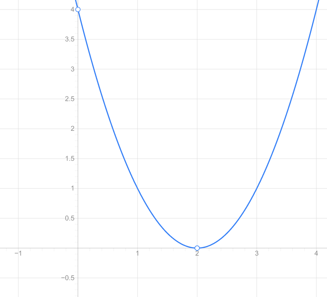
The graph reaches the x-axis but does not pass through it.
This behaviour is sometimes described as bouncing off the x-axis.
Multiplicity 3
Consider:
f(x) = (x − 2)³
The zero is:
x = 2
with multiplicity:
3
Because 3 is odd, the graph crosses the x-axis.
However, the graph becomes flatter near the root than it would for multiplicity 1.
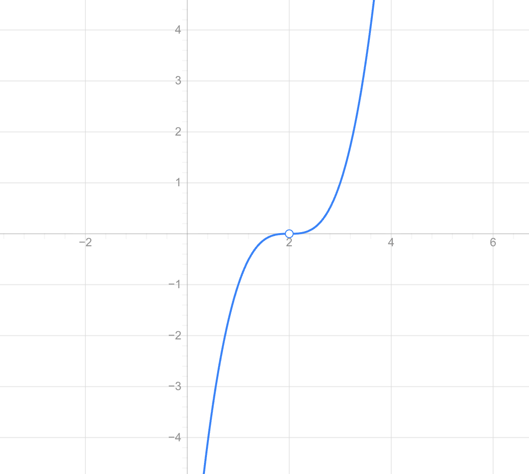
The graph still crosses, but it tends to flatten as it passes through the intercept.
Multiplicity 4
Consider:
f(x) = (x − 2)⁴
The zero is:
x = 2
with multiplicity:
4
Because 4 is even, the graph touches the x-axis and turns around.
Higher multiplicity also causes the graph to become flatter near the root.
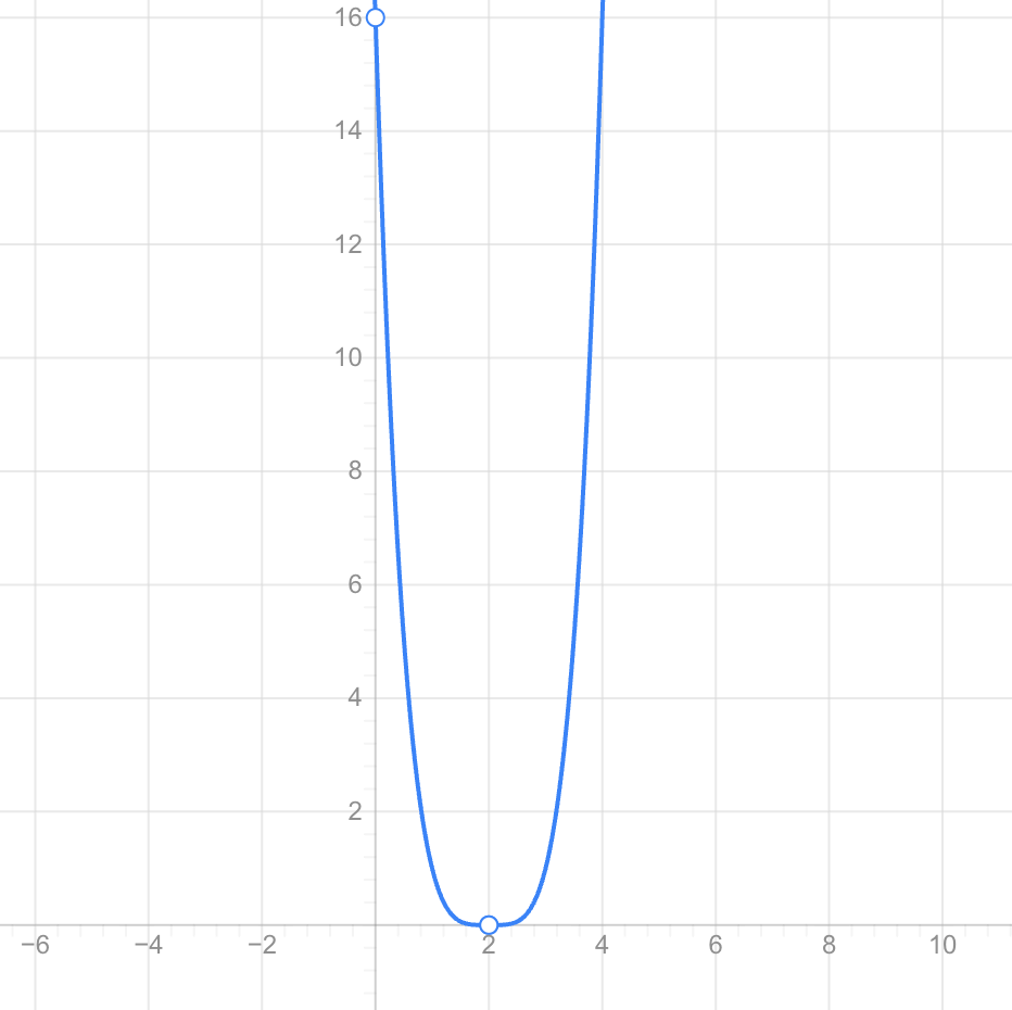
So multiplicity 4 behaves like multiplicity 2 in terms of crossing versus touching, but the graph is flatter near the zero.
Odd Multiplicity
Zeros with odd multiplicity cause the graph to cross the x-axis.
Examples include multiplicities:
1, 3, 5, 7, ...
The function changes sign as it passes through the root.
For example, it might change from:
negative → positive
or:
positive → negative


Even Multiplicity
Zeros with even multiplicity cause the graph to touch the x-axis and turn around.
Examples include:
2, 4, 6, 8, ...
The function does not change sign at the root.
If the graph approaches the x-axis from above, it touches the axis and returns upward.
If it approaches from below, it touches the axis and returns downward.
A Useful Multiplicity Pattern
When sketching, remember:
Multiplicity 1 → crosses
Multiplicity 2 → touches and turns
Multiplicity 3 → crosses and flattens
Multiplicity 4 → touches, turns, and flattens
For higher multiplicities, the same odd/even pattern continues.
The larger the multiplicity, the flatter the graph tends to become near the root.


Worked Example — Predicting Graph Behaviour
Consider:
f(x) = (x + 2)(x − 1)²
The zeros are:
x = −2
with multiplicity:
1
and:
x = 1
with multiplicity:
2
Therefore:
At:
x = −2
the graph crosses the x-axis.
At:
x = 1
the graph touches the x-axis and turns around.
This information already tells us a great deal about the shape of the graph.
Degree from Multiplicity
When a polynomial is completely factored, the multiplicities can help identify its degree.
Consider:
f(x) = (x + 3)²(x − 1)³
The first factor contributes degree:
2
The second contributes degree:
3
Therefore:
Degree = 2 + 3 = 5
This is a fifth-degree polynomial.
The sum of the multiplicities is:
5
Multiplicity and End Behaviour Together
To sketch a polynomial successfully, we can combine information about:
- Zeros
- Multiplicities
- Degree
- Leading coefficient
- End behaviour
Consider:
f(x) = (x + 2)(x − 1)²
The degree is:
1 + 2 = 3
So the polynomial has odd degree.
Its leading coefficient is positive.
Therefore:
Left end → down
Right end → up
At:
x = −2
the graph crosses.
At:
x = 1
the graph touches and turns.
Together, these facts give us the basic shape.
Sketching from Zeros and Multiplicity
A useful process is:
- Write down all zeros.
- Identify the multiplicity of each zero.
- Plot each zero on the x-axis.
- Determine whether the graph crosses or touches at each zero.
- Determine the degree.
- Determine the sign of the leading coefficient.
- Predict the end behaviour.
- Find the y-intercept if useful.
- Connect the features with a smooth curve.
Polynomial graphs should be drawn smoothly, without sharp corners.
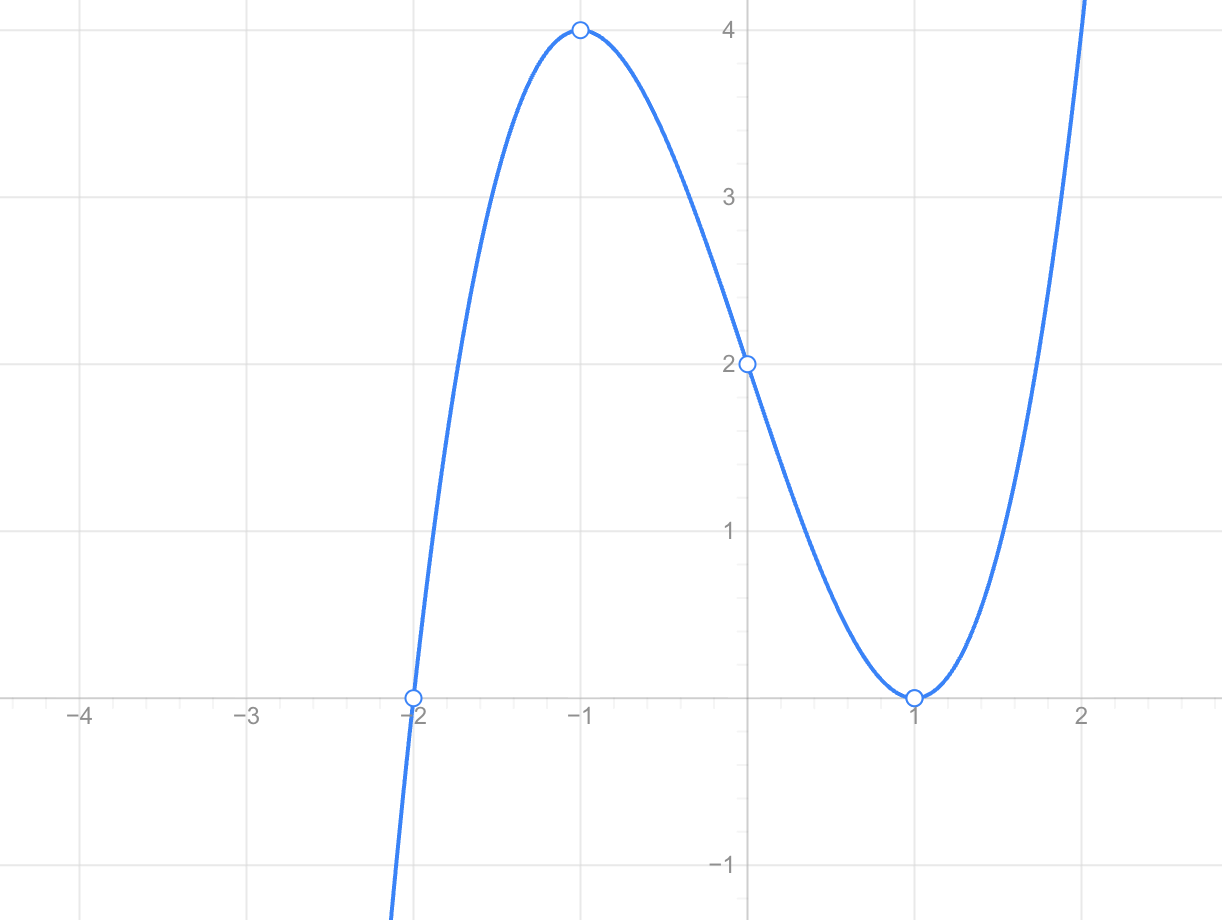
Worked Example — Sketching a Cubic
Sketch the general graph of:
f(x) = (x + 2)(x − 1)²
Zeros:
x = −2, multiplicity 1
x = 1, multiplicity 2
Degree:
3
Leading coefficient:
positive
End behaviour:
Left end → down
Right end → up
At:
x = −2
the graph crosses the x-axis.
At:
x = 1
the graph touches the x-axis and turns.
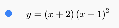


4. Transformations of Polynomial Functions
Learning outcomes
- I can identify vertical and horizontal translations.
- I can identify reflections and stretches.
- I can determine the effect of transformations on polynomial graphs.
- I can write transformed polynomial equations.
- I can sketch transformed polynomial functions.
Transformations of Polynomial Functions
A transformation changes the position, orientation, or shape of a graph without changing the basic family of function it belongs to.
For example, begin with the basic quadratic function:
f(x) = x²
We can move it up, down, left, or right. We can reflect it or stretch and compress it.
Examples include:
y = x² + 3
y = (x − 2)²
y = −x²
y = 3x²
Each equation is a transformation of the original function.


Learning Targets
- I can identify vertical and horizontal translations.
- I can identify reflections and stretches.
- I can determine the effect of transformations on polynomial graphs.
- I can write transformed polynomial equations.
- I can sketch transformed polynomial functions.
Parent Functions
A parent function is the simplest version of a particular family of functions.
Some common polynomial parent functions are:
Linear: f(x) = x
Quadratic: f(x) = x²
Cubic: f(x) = x³
Quartic: f(x) = x⁴
Transformations create new functions based on these basic graphs.


The General Transformation Form
A transformed function can often be written as:
g(x) = a f(b(x − h)) + k
Each value controls a different transformation.
h controls horizontal translation.
k controls vertical translation.
a controls vertical stretching, compression, and reflection across the x-axis.
b controls horizontal stretching, compression, and reflection across the y-axis.
Understanding these values allows us to predict a graph without plotting many individual points.
Vertical Translations
A vertical translation moves a graph upward or downward.
Starting with:
y = f(x)
the transformed function:
y = f(x) + k
moves the graph vertically.
If:
k > 0
the graph moves up.
If:
k < 0
the graph moves down.
Moving a Graph Up
Consider:
f(x) = x²
Now transform it to:
g(x) = x² + 3
Every y-value increases by 3.
Therefore, the entire graph moves:
3 units upward
The original vertex:
(0, 0)
becomes:
(0, 3)


Moving a Graph Down
Consider:
f(x) = x²
and:
g(x) = x² − 4
Every y-value decreases by 4.
Therefore, the graph moves:
4 units downward
The vertex moves from:
(0, 0)
to:
(0, −4)
The shape and orientation of the graph remain unchanged.
Horizontal Translations
Horizontal translations move graphs left or right.
Starting with:
y = f(x)
the transformation:
y = f(x − h)
moves the graph horizontally.
The direction can initially seem backwards.
f(x − h) → right by h
f(x + h) → left by h


Moving a Graph Right
Consider:
f(x) = x²
and:
g(x) = (x − 3)²
The graph moves:
3 units right
The vertex changes from:
(0, 0)
to:
(3, 0)
Notice that the equation contains:
x − 3
but the graph moves right.
Moving a Graph Left
Consider:
g(x) = (x + 2)²
We can think of this as:
g(x) = (x − (−2))²
Therefore, the graph moves:
2 units left
The vertex becomes:
(−2, 0)
Combining Horizontal and Vertical Translations
Transformations can occur together.
Consider:
g(x) = (x − 2)² + 3
Starting with:
f(x) = x²
the graph moves:
2 units right
and:
3 units up
The vertex moves from:
(0, 0)
to:
(2, 3)


Worked Example — Identifying a Translation
Describe the transformation:
g(x) = (x + 4)² − 2
Start with:
f(x) = x²
Inside the brackets:
x + 4
means:
4 units left
Outside the brackets:
−2
means:
2 units down
Therefore:
Left 4 and down 2
The vertex moves to:
(−4, −2)
Reflections Across the X-Axis
Multiplying the entire function by −1 reflects its graph across the x-axis.
Starting with:
y = f(x)
the reflection is:
y = −f(x)
For example:
f(x) = x²
becomes:
g(x) = −x²


Every point:
(x, y)
becomes:
(x, −y)
The upward-opening parabola becomes a downward-opening parabola.
Reflection of a Cubic Function
Consider:
f(x) = x³
Reflecting across the x-axis gives:
g(x) = −x³
The original graph has:
Left end → down
Right end → up
After reflection:
Left end → up
Right end → down
The entire graph has been flipped vertically.
Reflections Across the Y-Axis
Replacing x with −x reflects a graph across the y-axis.
Starting with:
y = f(x)
the transformed function is:
y = f(−x)
For example, consider:
f(x) = (x − 2)³
Then:
f(−x) = (−x − 2)³
produces a reflection across the y-axis.


Some Reflections Appear Unchanged
Consider:
f(x) = x²
Reflect across the y-axis:
f(−x) = (−x)²
But:
(−x)² = x²
Therefore, the graph looks unchanged.
This happens because:
f(x) = x²
is symmetric about the y-axis.
The same is true for:
x⁴, x⁶, x⁸, ...
Vertical Stretches
Consider:
y = a f(x)
If:
|a| > 1
the graph undergoes a vertical stretch.
For example:
f(x) = x²
and:
g(x) = 3x²
Every y-value is multiplied by 3.
A point:
(1, 1)
becomes:
(1, 3)
A point:
(2, 4)
becomes:
(2, 12)


For a parabola, this makes the graph appear narrower or steeper.
Vertical Compressions
If:
0 < |a| < 1
the graph undergoes a vertical compression.
For example:
g(x) = 0.5x²
Every y-value is multiplied by:
0.5
The graph appears wider or flatter than:
y = x²
The basic shape remains recognizable.
The Sign and Size of a
In:
g(x) = a f(x)
the value of a tells us two things.
If:
a < 0
the graph is reflected across the x-axis.
If:
|a| > 1
there is a vertical stretch.
If:
0 < |a| < 1
there is a vertical compression.
For example:
g(x) = −3x²
contains both:
Reflection across the x-axis
and:
Vertical stretch by factor 3
Worked Example — Reflection and Stretch
Describe:
g(x) = −2(x − 3)² + 5
Compare it with:
f(x) = x²
The:
−2
means:
Reflection across the x-axis
and:
Vertical stretch by factor 2
The:
x − 3
means:
3 units right
The:
+5
means:
5 units up
Therefore, the transformed parabola has its vertex at:
(3, 5)
and opens downward.
Horizontal Stretches and Compressions
Changes inside the function affect horizontal dimensions.
Consider:
g(x) = f(bx)
If:
|b| > 1
the graph undergoes a horizontal compression by factor:
1/|b|
If:
0 < |b| < 1
the graph undergoes a horizontal stretch.
The horizontal effect is reciprocal, which can make these transformations more difficult to recognize.


Worked Example — Horizontal Compression
Suppose:
f(x) = x³ − x
and:
g(x) = f(2x)
The input has been multiplied by:
2
Therefore, the graph is horizontally compressed by a factor of:
1/2
Features of the graph occur at half their original x-coordinates.
Worked Example — Horizontal Stretch
Suppose:
g(x) = f(x/3)
This can be written:
g(x) = f((1/3)x)
Since:
b = 1/3
the graph is horizontally stretched by a factor of:
3
Features become three times farther from the y-axis.
Combining Several Transformations
Consider:
g(x) = −2(x + 1)³ + 4
Start with:
f(x) = x³
Now identify each transformation.
x + 1
means:
1 unit left
The factor:
−2
means:
Reflection across the x-axis
and:
Vertical stretch by factor 2
Finally:
+4
means:
4 units up


Transforming Important Points
Instead of calculating many new points, we can transform points from the original graph.
For a transformation:
g(x) = a f(x − h) + k
a point:
(x, y)
on the original graph moves to:
(x + h, ay + k)
This provides a powerful way to sketch transformed functions.
Worked Example — Transforming Points
Suppose:
f(x) = x²
and:
g(x) = 2(x − 3)² + 1
A point on the parent function is:
(0, 0)
Apply the transformation.
Move right 3:
x = 3
Multiply the y-value by 2:
2(0) = 0
Move up 1:
y = 1
So:
(0, 0) → (3, 1)
Another parent point is:
(1, 1)
It becomes:
(4, 3)
because:
x: 1 + 3 = 4
and:
y: 2(1) + 1 = 3
Transformations and Zeros
Transformations can change the zeros of a polynomial.
Consider:
f(x) = x² − 4
Its zeros are:
x = −2 and x = 2
Now move the graph upward:
g(x) = x² − 4 + 4
which simplifies to:
g(x) = x²
The two original x-intercepts have moved until they meet at:
x = 0
The transformed graph now has one distinct real zero with multiplicity 2.
Transformations can therefore change where a graph intersects the axes.
Horizontal Translation of Zeros
Consider:
f(x) = (x − 1)(x + 2)
Its zeros are:
x = 1 and x = −2
Now translate the graph 3 units right:
g(x) = f(x − 3)
Every important feature moves 3 units right.
Therefore, the zeros become:
x = 4 and x = 1
This allows us to predict transformed roots without solving the new polynomial from the beginning.
Transformations and End Behaviour
Some transformations change end behaviour while others do not.
Translations do not change the fundamental end directions.
For example, moving a positive quartic left, right, up, or down still leaves:
Both ends → up
A reflection across the x-axis reverses the vertical end behaviour.
A positive quartic with:
Both ends → up
becomes a negative quartic with:
Both ends → down
Transformations and Multiplicity
Translations and stretches do not normally change the multiplicity pattern of roots.
If a graph originally touches and turns at a double root, a horizontal translation moves that behaviour to a new x-coordinate.
If a graph crosses and flattens at a root with multiplicity 3, translating the graph moves that feature without changing its basic crossing behaviour.
This makes transformations useful when sketching complicated polynomial functions from simpler ones.
Writing a Transformed Equation
Suppose:
f(x) = x²
and you are asked to:
- Move right 4
- Move down 2
Start with:
x²
Right 4 means replace x with:
x − 4
giving:
(x − 4)²
Down 2 means subtract 2:
(x − 4)² − 2
Therefore:
g(x) = (x − 4)² − 2
Worked Example — Writing from a Description
Start with:
f(x) = x³
Apply:
- Reflection across the x-axis
- Vertical stretch by factor 3
- Move left 2
- Move up 5
Left 2:
(x + 2)³
Vertical stretch:
3(x + 2)³
Reflect:
−3(x + 2)³
Move up:
−3(x + 2)³ + 5
Therefore:
g(x) = −3(x + 2)³ + 5
Sketching Transformed Polynomial Functions
A good sketching process is:
- Identify the parent function.
- Identify horizontal translations.
- Identify vertical translations.
- Identify reflections.
- Identify stretches or compressions.
- Locate important transformed points.
- Determine end behaviour.
- Draw a smooth curve consistent with all of these features.
You usually do not need to create a large table of values.
Worked Example — Sketching a Transformed Quadratic
Sketch:
g(x) = −(x − 2)² + 4
Start with:
f(x) = x²
Transformations:
Right 2
Reflect across the x-axis
Up 4
The original vertex:
(0, 0)
moves to:
(2, 4)
Because of the reflection, the parabola opens downward.


Worked Example — Sketching a Transformed Cubic
Consider:
g(x) = 2(x + 1)³ − 3
Start with:
f(x) = x³
Transformations:
Left 1
Vertical stretch by factor 2
Down 3
The central point:
(0, 0)
moves to:
(−1, −3)
The graph still has the general increasing cubic shape because there is no reflection.
Comparing Original and Transformed Graphs
A transformation is often easier to understand when the original and transformed graphs are shown together.
For example, compare:
f(x) = x²
with:
g(x) = −2(x − 3)² + 4
The second graph is:
- Shifted right
- Shifted up
- Reflected
- Vertically stretched
Yet it remains recognizable as a transformed quadratic.


Reading Transformations from an Equation
Consider:
g(x) = 4(x − 5)⁴ − 2
Identify each part.
4
means:
Vertical stretch by factor 4
x − 5
means:
5 units right
−2
means:
2 units down
The parent function is:
f(x) = x⁴
Because the coefficient 4 is positive, there is no reflection across the x-axis.
Reading Transformations from a Graph
You may also be given a parent graph and a transformed graph.
Look for:
- Has the graph moved horizontally?
- Has it moved vertically?
- Has it flipped?
- Has it become steeper or flatter?
- Have important points moved?
- Has the end behaviour reversed?
Comparing corresponding features can reveal the transformations.
A Useful Transformation Summary
f(x) + k
moves the graph:
up k units
f(x) − k
moves the graph:
down k units
f(x − h)
moves the graph:
right h units
f(x + h)
moves the graph:
left h units
−f(x)
reflects the graph:
across the x-axis
f(−x)
reflects the graph:
across the y-axis
a f(x), |a| > 1
produces a:
vertical stretch
a f(x), 0 < |a| < 1
produces a:
vertical compression
Why Horizontal Changes Seem Backwards
One of the most common difficulties with transformations is horizontal translation.
Why does:
f(x − 3)
move the graph right rather than left?
Suppose an important feature originally occurs when:
x = 0
For the transformed function, the same input to f occurs when:
x − 3 = 0
Therefore:
x = 3
The feature has moved from:
x = 0
to:
x = 3
So the graph moves right.
Polynomial Transformations in Real Applications
Transformations are useful whenever a mathematical model needs to be adjusted.
They can represent:
- Changes in starting position
- Changes in baseline values
- Reversed relationships
- Increased or decreased scale
- Shifts in experimental data
- Adjustments to mathematical models
- Changes in computer-generated curves


The same transformation ideas are also fundamental in physics, engineering, computer graphics, and data analysis.
Common Mistakes
Mistake: Reversing Horizontal Translation
f(x − 3) means:
Right 3
not left 3.
f(x + 3) means:
Left 3
not right 3.
Mistake: Confusing Horizontal and Vertical Changes
Changes outside the function generally affect vertical position or scale.
Changes inside the function generally affect horizontal position or scale.
Mistake: Missing a Reflection
In:
−(x − 2)²
the negative sign outside the brackets reflects the graph across the x-axis.
Mistake: Treating a Vertical Stretch as a Translation
In:
3x²
the graph is not moved upward by 3.
Its y-values are multiplied by 3.
Mistake: Applying Horizontal Scale Directly
For:
f(2x)
the horizontal scale factor is:
1/2
not 2.
Mistake: Forgetting That Transformations Can Combine
A function such as:
−2(x + 3)⁴ + 5
contains several transformations at once.
Analyze each part separately.
Key Terms
Transformation – a change to the position, orientation, or scale of a graph.
Parent function – the simplest function in a particular family.
Translation – movement of a graph without changing its shape.
Vertical translation – movement upward or downward.
Horizontal translation – movement left or right.
Reflection – flipping a graph across an axis.
Vertical stretch – multiplying y-values so they move farther from the x-axis.
Vertical compression – multiplying y-values so they move closer to the x-axis.
Horizontal stretch – spreading a graph horizontally.
Horizontal compression – squeezing a graph horizontally.
Check Your Understanding
1. Describe the transformation from:
f(x) = x²
to:
g(x) = x² + 5
2. Describe:
g(x) = (x − 4)²
3. Describe:
g(x) = (x + 3)² − 2
4. What transformation occurs in:
g(x) = −x³
5. Describe the transformations in:
g(x) = 3x²
6. Describe the transformations in:
g(x) = −2x⁴
7. Describe:
g(x) = 2(x − 3)² + 5
8. Describe:
g(x) = −3(x + 2)³ − 4
9. Write an equation obtained by moving:
f(x) = x²
4 units right and 6 units up.
10. Write an equation obtained by moving:
f(x) = x³
2 units left and 5 units down.
11. Write an equation for a reflection of:
f(x) = x⁴
across the x-axis.
12. Write an equation for a vertical stretch of:
f(x) = x²
by a factor of 5.
13. Explain why:
f(x − 3)
moves a graph right rather than left.
14. Describe the effect of:
g(x) = f(2x)
on the graph of f(x).
15. Explain how you would sketch:
g(x) = −2(x − 1)⁴ + 3
starting from the graph of:
f(x) = x⁴
Key Takeaways
- Transformations change the position, orientation, or scale of polynomial graphs.
- f(x) + k moves a graph vertically.
- f(x − h) moves a graph horizontally.
- Horizontal translations appear to work in the opposite direction from the sign inside the brackets.
- −f(x) reflects a graph across the x-axis.
- f(−x) reflects a graph across the y-axis.
- Multiplying a function by a number greater than 1 produces a vertical stretch.
- Multiplying by a number between 0 and 1 produces a vertical compression.
- Changes inside the function can create horizontal stretches or compressions.
- Several transformations can occur in the same equation.
- Important points can be transformed instead of recalculated from the beginning.
- Transformations can affect zeros and intercepts.
- Reflections can change end behaviour.
- Translations do not change the fundamental degree or basic polynomial family.
- Recognizing transformations allows complicated polynomial graphs to be sketched efficiently.
Did You Know?
Graph transformations are not limited to algebra. The same basic ideas—translation, reflection, stretching, and compression—are used extensively in computer graphics and animation. When an object on a screen is moved, flipped, or resized, the software performs mathematical transformations closely related to the transformations used to move and reshape function graphs.
5. Modelling with Polynomial Functions
Learning outcomes
- I can identify situations modelled by polynomial functions.
- I can interpret polynomial models in context.
- I can estimate values using polynomial graphs.
- I can evaluate polynomial functions for given inputs.
- I can solve real-world problems involving polynomial models.


