Non-Linear Functions
| Website: | Young Education |
| Kurs: | Functions and Graphs |
| Buch: | Non-Linear Functions |
| Gedruckt von: | Guest user |
| Datum: | Montag, 9. November 2026, 16:36 |
1. Quadratic Functions
Learning outcomes
- I can recognize quadratic functions.
- I can identify parabolic graphs.
- I can describe the shape of quadratic graphs.
- I can compare linear and quadratic functions.
- I can interpret quadratic relationships.


2. Exponential Functions
Learning outcomes
- I can recognize exponential growth.
- I can recognize exponential decay.
- I can compare exponential and linear growth.
- I can interpret exponential graphs.
- I can identify real-life exponential relationships.
Exponential Functions
An exponential function describes a relationship in which a quantity changes by the same factor or percentage over equal intervals.
A common form is:
y = abˣ
where:
- a = initial value
- b = growth or decay factor
- x = independent variable
- y = dependent variable
The important feature is that the variable x appears in the exponent.
For example:
y = 3(2ˣ)
is exponential because x is an exponent.
By contrast:
y = 3x + 2
is linear because x is multiplied by a constant.


Recognizing an Exponential Function
Consider:
y = 5(2ˣ)
The variable x appears in the exponent.
Therefore this is an exponential function.
Now consider:
y = 5x²
Here x is the base and 2 is the exponent.
This is quadratic, not exponential.
The position of the variable matters.
Exponential Growth
An exponential function represents growth when its values repeatedly multiply by a factor greater than 1.
For:
y = abˣ
exponential growth occurs when:
b > 1
For example:
y = 100(2ˣ)
has:
a = 100
b = 2
The quantity doubles every time x increases by 1.
A Growth Table
Consider:
y = 2ˣ
| x | y |
|---|---|
| 0 | 1 |
| 1 | 2 |
| 2 | 4 |
| 3 | 8 |
| 4 | 16 |
| 5 | 32 |
Notice:
1 → 2 → 4 → 8 → 16 → 32
Each value is multiplied by:
2
This constant multiplication factor is the key sign of an exponential relationship.
Constant Factor Rather Than Constant Difference
For exponential functions, look for a constant ratio between consecutive outputs.
In:
3, 6, 12, 24, 48
each value is:
2 times the previous value
Therefore:
growth factor = 2
Compare this with:
3, 6, 9, 12, 15
Here we repeatedly add 3.
That is a linear pattern.
Exponential Decay
An exponential function represents decay when the quantity repeatedly decreases by the same percentage or multiplication factor.
For:
y = abˣ
decay occurs when:
0 < b < 1
For example:
y = 100(0.5ˣ)
means the quantity is multiplied by:
0.5
each interval.
In other words, it halves each time.


A Decay Table
Consider:
y = 80(0.5ˣ)
| x | y |
|---|---|
| 0 | 80 |
| 1 | 40 |
| 2 | 20 |
| 3 | 10 |
| 4 | 5 |
The values are:
80 → 40 → 20 → 10 → 5
Each value is half the previous value.
The decay factor is:
0.5
Initial Value
In:
y = abˣ
the value a represents the initial value when:
x = 0
This works because:
b⁰ = 1
Therefore:
y = a(1)
y = a
For:
y = 250(1.4ˣ)
the initial value is:
250
The graph passes through:
(0, 250)
Growth Factor
In:
y = abˣ
the value b is the growth factor or decay factor.
For:
y = 50(3ˣ)
the growth factor is:
3
The quantity triples every interval.
For:
y = 50(0.8ˣ)
the decay factor is:
0.8
The quantity retains 80% of its previous value each interval.
Growth Rate as a Percentage
Suppose a quantity increases by:
20%
each year.
The original amount represents:
100%
After the increase, it becomes:
120%
As a decimal:
120% = 1.20
Therefore the growth factor is:
1.20
The model has the form:
y = a(1.20ˣ)
Growth Factor Formula
If the growth rate is r as a decimal:
growth factor = 1 + r
For example:
10% growth:
b = 1 + 0.10 = 1.10
25% growth:
b = 1 + 0.25 = 1.25
4% growth:
b = 1 + 0.04 = 1.04
Decay Factor from a Percentage
Suppose a quantity decreases by:
20%
each year.
It retains:
80%
of its previous value.
Therefore:
b = 0.80
The model has the form:
y = a(0.80ˣ)
Decay Factor Formula
If the decay rate is r:
decay factor = 1 − r
For example:
10% decrease:
b = 1 − 0.10 = 0.90
25% decrease:
b = 1 − 0.25 = 0.75
60% decrease:
b = 1 − 0.60 = 0.40
Growth Rate Is Not the Same as Growth Factor
This distinction is important.
If something increases by:
15%
then:
growth rate = 15% = 0.15
but:
growth factor = 1.15
For:
y = 500(1.15ˣ)
the number:
1.15
does not mean 115% growth.
It means the quantity retains its original 100% and gains an additional 15%.
Decay Rate Is Not the Same as Decay Factor
For:
y = 500(0.85ˣ)
the decay factor is:
0.85
This means:
85% remains
so:
15% is lost
each interval.
Therefore:
decay rate = 15%
Shape of an Exponential Growth Graph
An exponential growth graph typically:
- increases slowly at first
- becomes increasingly steep
- rises rapidly for larger x-values
- curves upward
Unlike a linear graph, it does not increase by equal amounts over equal intervals.


Shape of an Exponential Decay Graph
An exponential decay graph typically:
- decreases quickly at first
- decreases more slowly later
- approaches zero
- does not normally reach zero in the basic mathematical model
This produces a curved graph that becomes flatter over time.
Horizontal Asymptote
For basic exponential functions such as:
y = 2ˣ
and:
y = 0.5ˣ
the graph approaches:
y = 0
but does not reach it.
The line:
y = 0
is called a horizontal asymptote.
An asymptote is a line that a graph approaches increasingly closely.
Exponential Functions Are Not Straight Lines
Consider:
y = 2ˣ
The slope is constantly changing.
As x increases, the graph becomes steeper.
Therefore the graph is curved.
This differs fundamentally from a linear function, which has a constant slope.
Linear Growth
A linear function has the form:
y = mx + b
Linear growth involves adding the same amount during each interval.
For example:
100, 120, 140, 160, 180
Each value increases by:
20
The difference is constant.
Exponential Growth
Exponential growth involves multiplying by the same factor.
For example:
100, 120, 144, 172.8, 207.36
Each value is multiplied by:
1.2
This represents:
20% growth
during each interval.
The amount being added gets larger because 20% is being calculated from an increasingly large quantity.
Linear Versus Exponential Growth
Suppose two quantities both begin at 100.
Linear:
L = 100 + 20x
Exponential:
E = 100(1.2ˣ)
| x | Linear | Exponential |
|---|---|---|
| 0 | 100 | 100 |
| 1 | 120 | 120 |
| 2 | 140 | 144 |
| 3 | 160 | 172.8 |
| 4 | 180 | 207.36 |
| 5 | 200 | 248.83 |
At first, the values may appear similar.
Over time, the exponential function grows much faster.


Why Exponential Growth Becomes So Fast
Suppose a population increases by:
10% each year
The increase itself becomes larger every year.
If the population is:
1,000
the first increase is:
100
giving:
1,100
The next 10% increase is based on 1,100:
110
giving:
1,210
The next increase is:
121
The quantity being added is itself increasing.
This is the key reason exponential growth can become extremely rapid.
Repeated Addition Versus Repeated Multiplication
This provides a useful recognition rule.
Linear
Repeated addition:
5, 8, 11, 14, 17
Add:
3
each time.
Exponential
Repeated multiplication:
5, 10, 20, 40, 80
Multiply by:
2
each time.
Think:
Linear → constant difference
Exponential → constant ratio
Recognizing Exponential Functions from Tables
Consider:
| x | y |
|---|---|
| 0 | 4 |
| 1 | 12 |
| 2 | 36 |
| 3 | 108 |
| 4 | 324 |
Calculate consecutive ratios:
12/4 = 3
36/12 = 3
108/36 = 3
324/108 = 3
The ratio is constant.
Therefore the relationship is exponential.
The model is:
y = 4(3ˣ)
Recognizing Exponential Decay from Tables
Consider:
| x | y |
|---|---|
| 0 | 160 |
| 1 | 80 |
| 2 | 40 |
| 3 | 20 |
| 4 | 10 |
Ratios:
80/160 = 0.5
40/80 = 0.5
20/40 = 0.5
10/20 = 0.5
The constant ratio is:
0.5
Therefore this is exponential decay.
Linear, Quadratic, and Exponential Tables
These patterns can often be distinguished by their differences or ratios.
Linear
Constant first difference
Example:
2, 5, 8, 11, 14
Quadratic
Constant second difference
Example:
0, 1, 4, 9, 16
Exponential
Constant ratio
Example:
2, 6, 18, 54, 162
This is an extremely useful recognition strategy.
A Comparison Table
| Feature | Linear | Quadratic | Exponential |
|---|---|---|---|
| Example | y = 2x + 1 | y = x² | y = 2ˣ |
| Variable | Power 1 | Power 2 | In exponent |
| Graph | Straight line | Parabola | Exponential curve |
| Pattern | Constant difference | Constant second difference | Constant ratio |
| Rate of change | Constant | Changes steadily | Changes multiplicatively |
| Typical growth | Add same amount | Increasing differences | Multiply by same factor |
Population Growth
Populations can sometimes grow approximately exponentially when the percentage growth rate remains relatively constant.
Suppose a bacterial population begins with:
500 bacteria
and increases by:
20% each hour
The growth factor is:
1.20
Model:
P = 500(1.2ᵗ)
where t is time in hours.
After 4 hours:
P = 500(1.2⁴)
P = 500(2.0736)
P = 1036.8
The model predicts approximately:
1,037 bacteria


Doubling
A common exponential growth pattern is doubling.
Suppose a cell population doubles every hour.
Starting with:
200 cells
the pattern is:
200 → 400 → 800 → 1600 → 3200
The model is:
P = 200(2ᵗ)
The factor 2 represents doubling.
Compound Interest
Money invested with compound interest can grow exponentially.
Suppose $1,000 grows by:
5% per year
The growth factor is:
1.05
Model:
A = 1000(1.05ᵗ)
After 10 years:
A = 1000(1.05¹⁰)
Approximately:
A = $1,628.89
The interest earned in earlier years also earns interest in later years.
This is why compound interest is exponential rather than linear.
Simple Versus Compound Growth
If $100 is added to an account every year:
linear growth
because the same amount is added.
If the account increases by 5% every year:
exponential growth
because the same percentage is applied repeatedly.
The wording of a problem often reveals the type of relationship.
Inflation
If prices increase by approximately the same percentage each year, an exponential model may be useful.
For example, if a price begins at $200 and increases by 3% annually:
P = 200(1.03ᵗ)
This does not mean exactly $6 is added every year.
The amount added increases as the price becomes larger.
Radioactive Decay
Radioactive materials decrease exponentially.
Suppose a sample contains:
800 mg
and half remains after each half-life.
The pattern is:
800 → 400 → 200 → 100 → 50
A simple model using n as the number of half-lives is:
M = 800(0.5ⁿ)
This is exponential decay.


Half-Life
Half-life is the time required for half of a quantity to decay.
After:
1 half-life → 1/2 remains
2 half-lives → 1/4 remains
3 half-lives → 1/8 remains
4 half-lives → 1/16 remains
The same fraction disappears repeatedly, producing exponential decay.
Depreciation
The value of some products decreases by a percentage each year.
Suppose a car is worth:
$30,000
and loses:
15% of its value each year
It retains:
85%
Therefore:
V = 30000(0.85ᵗ)
After one year:
V = $25,500
After another year, the 15% decrease is calculated from $25,500 rather than the original $30,000.
This produces exponential decay.
Medication in the Body
Some medications are removed from the body at approximately exponential rates.
If 80% remains after each hour, then:
decay factor = 0.80
Starting with 200 mg:
A = 200(0.8ᵗ)
The amount decreases rapidly at first and more slowly later.
Cooling and Exponential Relationships
Under suitable conditions, the difference between an object's temperature and its surroundings can decrease approximately exponentially.
This means cooling does not necessarily occur by exactly the same number of degrees each minute.
The temperature often changes rapidly at first and more slowly as it approaches the surrounding temperature.
This is another example of exponential decay toward a limiting value.
Interpreting Exponential Graphs
When examining an exponential graph, look for:
- initial value
- growth or decay
- rate or factor
- direction of change
- steepness
- asymptotic behaviour
- meaningful domain
- real-world interpretation
The shape of the graph provides important information about the relationship.
Reading the Initial Value
For:
y = 300(1.4ˣ)
when:
x = 0
y = 300
Therefore the graph crosses the y-axis at:
(0, 300)
This represents the initial quantity.
Reading Growth from a Graph
If an exponential graph increases:
- slowly at first
- then increasingly rapidly
it may represent exponential growth.
If equal horizontal intervals correspond to multiplication by approximately the same factor, this provides stronger evidence.
Reading Decay from a Graph
If a graph:
- decreases rapidly initially
- becomes increasingly flat
- approaches a horizontal value
it may represent exponential decay.
The graph's behaviour reflects repeated percentage or proportional change.
Exponential Models and Asymptotes
Consider:
y = 100(0.5ˣ)
As x increases:
y gets closer and closer to 0
but the basic mathematical function does not reach zero for any finite x.
This is different from a linear decay model such as:
y = 100 − 10x
which reaches zero exactly when:
x = 10
Comparing Linear and Exponential Decay
Linear decay:
100, 90, 80, 70, 60
Subtract:
10
each time.
Exponential decay:
100, 90, 81, 72.9, 65.61
Multiply by:
0.9
each time.
Linear decay removes the same amount.
Exponential decay removes the same percentage.
Predicting Values
Suppose:
P = 200(1.5ᵗ)
Predict P when:
t = 4
Substitute:
P = 200(1.5⁴)
P = 200(5.0625)
P = 1012.5
The model predicts approximately:
1,013
if the quantity must be a whole number.
Working Backwards Conceptually
Suppose:
P = 100(2ᵗ)
The values are:
t = 0 → 100
t = 1 → 200
t = 2 → 400
t = 3 → 800
If:
P = 800
we can recognize:
t = 3
More advanced exponential equations may require logarithms to solve when the answer cannot be identified easily.
Comparing Two Exponential Functions
Consider:
A = 100(1.1ˣ)
B = 100(1.3ˣ)
Both begin at:
100
But B has the larger growth factor.
Therefore B grows faster for positive x.
The difference between them becomes increasingly large over time.
Same Growth Factor, Different Initial Values
Consider:
A = 100(1.2ˣ)
B = 500(1.2ˣ)
Both grow by:
20% per interval
but B begins five times larger.
In fact, B remains five times A for every x-value.
Comparing Growth Rates Carefully
Consider:
A = 100(1.10ˣ)
B = 20(1.30ˣ)
A begins much larger.
B grows faster.
Therefore A may initially have the greater value, while B may eventually overtake it.
When comparing exponential functions, consider both:
- initial value
- growth factor
Exponential Models Have Limits
A mathematical exponential function may continue indefinitely.
Real systems usually cannot.
A bacterial population cannot grow exponentially forever because eventually there may be shortages of:
- food
- space
- oxygen
- other resources
Therefore exponential growth may be a good model only over a limited interval.
Population Growth Is Not Always Exponential
Real populations may initially grow approximately exponentially.
Later, growth may slow because of:
- limited resources
- disease
- competition
- environmental changes
- migration
A different model may then become more appropriate.
Mathematical models must always be evaluated against reality.
Exponential Relationships in Science
Exponential functions appear in many scientific contexts, including:
- radioactive decay
- population growth
- bacterial growth
- charging and discharging processes
- attenuation
- some cooling processes
- drug elimination
- chain reactions
Recognizing exponential behaviour helps scientists make predictions about rapidly changing systems.
Exponential Relationships in Finance
Exponential functions are also important in:
- compound interest
- inflation
- investment growth
- depreciation
- debt growth
Small percentage changes repeated many times can produce large long-term effects.
This is one reason exponential growth is so important in financial decision-making.
Recognizing Exponential Relationships from Words
Words suggesting exponential growth include:
- doubles every...
- triples every...
- increases by 5% each...
- grows by 20% per...
- multiplied by...
Words suggesting exponential decay include:
- halves every...
- loses 10% each...
- decreases by 25% per...
- retains 80% each...
- decays by...
The key idea is repeated multiplication, not repeated addition or subtraction.
A Reliable Recognition Strategy
Use:
Equation → Table → Graph → Context
Equation
Is the variable in the exponent?
Table
Is there approximately a constant ratio between outputs for equally spaced inputs?
Graph
Does it show the characteristic exponential growth or decay curve?
Context
Does the situation involve repeated percentage or proportional change?
Using several types of evidence gives a stronger conclusion.
Linear, Quadratic, or Exponential?
Ask:
Is there a constant first difference?
Likely:
Linear
Is there a constant second difference?
Likely:
Quadratic
Is there a constant ratio?
Likely:
Exponential
This applies when the x-values are equally spaced.
Common Mistakes
Mistake: Thinking y = x² is exponential.
The variable is the base, not the exponent.
y = x² is quadratic.
Mistake: Thinking y = 2ˣ is quadratic.
The variable appears in the exponent.
Therefore it is exponential.
Mistake: Looking for a constant difference in an exponential table.
Look for a constant ratio.
Mistake: Confusing growth rate and growth factor.
20% growth gives:
growth rate = 0.20
growth factor = 1.20
Mistake: Using 0.20 as the factor for 20% growth.
That would mean only 20% remains each interval.
For 20% growth, use:
1.20
Mistake: Using 1.20 for 20% decay.
For 20% decay:
80% remains
so use:
0.80
Mistake: Thinking exponential growth adds the same amount each time.
It multiplies by the same factor.
Mistake: Thinking exponential decay subtracts the same amount each time.
It usually decreases by the same percentage or factor.
Mistake: Assuming exponential decay reaches zero quickly.
Basic exponential decay approaches zero asymptotically.
Mistake: Assuming exponential growth can continue forever in real systems.
Resources and physical limitations often restrict exponential growth.
Mistake: Comparing exponential models using only their initial values.
The growth factors must also be considered.
Mistake: Assuming every rapidly increasing graph is exponential.
Check the equation, ratios, and context before classifying the relationship.
Key Terms
Exponential function — function in which the independent variable appears in an exponent.
Exponential growth — repeated proportional increase represented by a growth factor greater than 1.
Exponential decay — repeated proportional decrease represented by a factor between 0 and 1.
Initial value — starting amount, represented by a in y = abˣ.
Growth factor — multiplier greater than 1 applied during each interval.
Decay factor — multiplier between 0 and 1 applied during each interval.
Growth rate — percentage by which a quantity increases during each interval.
Decay rate — percentage by which a quantity decreases during each interval.
Constant ratio — same quotient between consecutive outputs for equally spaced inputs.
Linear growth — growth involving a constant additive change.
Compound growth — growth in which increases are repeatedly applied to the new total.
Compound interest — interest calculated on both the original amount and previously accumulated interest.
Depreciation — decrease in value over time.
Half-life — time required for half of a quantity to decay.
Asymptote — line that a graph approaches increasingly closely.
Horizontal asymptote — horizontal line approached by a graph.
Interpolation — prediction within the range of known data.
Extrapolation — prediction beyond the range of known data.
Exponential model — exponential function used to represent a real situation.
Key Takeaways
- Exponential functions have the variable in the exponent.
- A common form is y = abˣ.
- The value a represents the initial amount.
- The value b represents the growth or decay factor.
- If b > 1, the function represents exponential growth.
- If 0 < b < 1, the function represents exponential decay.
- Exponential growth involves repeated multiplication by a factor greater than 1.
- Exponential decay involves repeated multiplication by a factor between 0 and 1.
- Linear relationships have constant differences.
- Exponential relationships have constant ratios for equally spaced inputs.
- Quadratic relationships have constant second differences for equally spaced inputs.
- Linear growth repeatedly adds the same amount.
- Exponential growth repeatedly multiplies by the same factor.
- Percentage growth produces exponential relationships when the percentage is repeatedly applied.
- A growth rate r gives a factor of 1 + r.
- A decay rate r gives a factor of 1 − r.
- A 20% increase corresponds to a factor of 1.20.
- A 20% decrease corresponds to a factor of 0.80.
- Exponential growth graphs become increasingly steep.
- Exponential decay graphs decrease rapidly at first and then flatten.
- Basic exponential growth and decay functions commonly have a horizontal asymptote at y = 0.
- Exponential growth can eventually exceed linear growth dramatically.
- Exponential relationships occur in population growth, bacterial growth, compound interest, inflation, and other situations.
- Exponential decay occurs in radioactive decay, depreciation, medication elimination, and other processes.
- Real-world exponential models are usually valid only over an appropriate range.
- Equations, tables, graphs, and context can all help identify exponential relationships.
Check Your Understanding
- What feature of an equation usually identifies it as exponential?
- Which is exponential: y = x², y = 2x, or y = 2ˣ? Explain.
- In y = 300(1.4ˣ), identify the initial value and growth factor.
- Does y = 500(0.75ˣ) represent growth or decay? Explain.
- A population increases by 12% each year. What is its growth factor?
- A machine loses 8% of its value each year. What is its decay factor?
- Explain the difference between a growth rate and a growth factor.
- Determine whether 5, 10, 20, 40, 80 represents a linear or exponential pattern. Explain.
- Determine whether 5, 10, 15, 20, 25 represents a linear or exponential pattern. Explain.
- Determine whether 160, 80, 40, 20, 10 represents exponential growth or decay and identify the factor.
- Compare the meaning of constant difference and constant ratio.
- A bacteria culture begins with 400 bacteria and doubles every hour. Write an exponential model for the population after t hours.
- Use your model from Question 12 to predict the population after 6 hours.
- An investment of $2,000 increases by 5% annually. Write an exponential model for its value after t years.
- A car worth $40,000 loses 12% of its value each year. Write an exponential model for its value.
- Explain why compound interest is exponential rather than linear.
- Explain how the graph of exponential growth differs from a straight-line graph.
- Explain why an exponential decay graph can approach zero without reaching zero in the basic model.
- Compare A = 100(1.1ˣ) and B = 100(1.25ˣ). Which begins larger? Which grows faster? Explain.
- Give one real-world example of exponential growth and one example of exponential decay. For each, explain what is repeatedly multiplied, identify a possible growth or decay factor, and describe one reason the exponential model might eventually stop being appropriate.
3. Piecewise and Step Functions
Learning outcomes
- I can recognize piecewise functions.
- I can interpret step graphs.
- I can determine outputs from piecewise graphs.
- I can explain why piecewise functions are useful.
- I can describe real-life examples.


4. Comparing Function Types
Learning outcomes
- I can distinguish between linear, quadratic, and exponential functions.
- I can compare their graphs.
- I can compare rates of change.
- I can identify each function from data.
- I can determine which model best fits a situation.
Comparing Function Types
Functions describe relationships between quantities. Three of the most important types of functions are linear, quadratic, and exponential functions.
Although all three can be represented using equations, tables, and graphs, they behave very differently.
Learning to recognize these differences allows us to choose an appropriate mathematical model for a real-world situation.
Linear Functions
A linear function has a constant rate of change.
A common form is:
y = mx + b
where:
- m = slope or rate of change
- b = y-intercept
For example:
y = 2x + 1
Every time x increases by 1, y increases by 2.
| x | y |
|---|---|
| 0 | 1 |
| 1 | 3 |
| 2 | 5 |
| 3 | 7 |
| 4 | 9 |
The first differences are:
+2, +2, +2, +2
Because the first differences are constant, the relationship is linear.
Graph Shape
The graph of a linear function is a straight line.
A positive slope produces an increasing line, while a negative slope produces a decreasing line.


Linear relationships appear when something changes by the same amount during each equal interval.
Examples include:
- Earning the same amount of money each hour
- Travelling at constant speed
- Filling a container at a constant rate
- Paying a fixed price per item
Quadratic Functions
A quadratic function contains a squared variable.
A common form is:
y = ax² + bx + c
where a ≠ 0.
For example:
y = x²
| x | y |
|---|---|
| 0 | 0 |
| 1 | 1 |
| 2 | 4 |
| 3 | 9 |
| 4 | 16 |
The first differences are:
+1, +3, +5, +7
These are not constant.
However, the second differences are:
+2, +2, +2
Constant second differences are an important clue that a table represents a quadratic function when the x-values increase by equal amounts.
Graph Shape
The graph of a quadratic function is called a parabola.


A parabola can open upward or downward.
If a > 0, it opens upward.
If a < 0, it opens downward.
The turning point of a parabola is called its vertex.
Quadratic relationships appear in situations involving:
- Projectile motion
- Falling objects
- Areas of geometric shapes
- Optimization problems
- Some profit and revenue models
Exponential Functions
An exponential function changes by a constant multiplying factor rather than a constant amount.
A common form is:
y = abˣ
where:
- a = initial value
- b = growth or decay factor
For example:
y = 2ˣ
| x | y |
|---|---|
| 0 | 1 |
| 1 | 2 |
| 2 | 4 |
| 3 | 8 |
| 4 | 16 |
Each output is multiplied by 2:
1 → 2 → 4 → 8 → 16
The ratio between consecutive outputs is constant:
2/1 = 2
4/2 = 2
8/4 = 2
16/8 = 2
This constant ratio is a major clue that a relationship is exponential.
Graph Shape
An exponential growth graph begins relatively slowly and then becomes increasingly steep.


If:
b > 1
the function represents exponential growth.
If:
0 < b < 1
the function represents exponential decay.
Exponential relationships appear in situations involving:
- Population growth
- Compound interest
- Bacterial growth
- Radioactive decay
- Depreciation
- Spread of information under simplified conditions
Comparing the Graphs
The shapes of the graphs provide one of the easiest ways to distinguish the three function types.
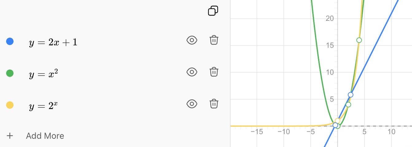
The three graphs have very different characteristics.
| Function Type | Typical Graph |
|---|---|
| Linear | Straight line |
| Quadratic | Parabola |
| Exponential | Increasing or decreasing curve |
Linear
A linear graph changes at a constant rate.
Its steepness remains constant.
Quadratic
A quadratic graph curves and has a turning point called the vertex.
Its rate of change changes steadily.
Exponential
An exponential graph becomes increasingly steep during growth or increasingly flat during decay.
Its rate of change depends on its current value.
Comparing Rates of Change
One of the most important differences between these functions is how their outputs change.
Linear: Constant Difference
Consider:
2, 5, 8, 11, 14
The differences are:
+3, +3, +3, +3
The output increases by the same amount each time.
This indicates a linear relationship.
Quadratic: Constant Second Difference
Consider:
1, 4, 9, 16, 25
First differences:
+3, +5, +7, +9
The first differences are not constant.
Now calculate the second differences:
+2, +2, +2
The second differences are constant.
This indicates a quadratic relationship.
Exponential: Constant Ratio
Consider:
3, 6, 12, 24, 48
Calculate the ratios:
6 ÷ 3 = 2
12 ÷ 6 = 2
24 ÷ 12 = 2
48 ÷ 24 = 2
Each output is multiplied by 2.
This indicates an exponential relationship.
A Useful Recognition Strategy
When x-values increase by equal amounts, look for these patterns:
| Pattern in y-values | Likely Function |
|---|---|
| Constant first difference | Linear |
| Constant second difference | Quadratic |
| Constant ratio | Exponential |
This provides a powerful way to identify functions from tables.
A useful memory aid is:
Linear → add
Quadratic → second differences
Exponential → multiply
Identifying Functions from Data
Suppose we have the following data.
Table A
| x | y |
|---|---|
| 0 | 5 |
| 1 | 8 |
| 2 | 11 |
| 3 | 14 |
| 4 | 17 |
Differences:
+3, +3, +3, +3
Therefore:
Linear
Table B
| x | y |
|---|---|
| 0 | 1 |
| 1 | 4 |
| 2 | 9 |
| 3 | 16 |
| 4 | 25 |
First differences:
+3, +5, +7, +9
Second differences:
+2, +2, +2
Therefore:
Quadratic
Table C
| x | y |
|---|---|
| 0 | 5 |
| 1 | 10 |
| 2 | 20 |
| 3 | 40 |
| 4 | 80 |
Ratios:
10 ÷ 5 = 2
20 ÷ 10 = 2
40 ÷ 20 = 2
80 ÷ 40 = 2
Therefore:
Exponential
Comparing Linear and Exponential Growth
Linear and exponential growth can look surprisingly similar at first.
Suppose two savings accounts begin with $100.
Account A
The balance increases by $100 each year.
100 → 200 → 300 → 400 → 500
This is linear growth because we repeatedly add the same amount.
Account B
The balance doubles each year.
100 → 200 → 400 → 800 → 1600
This is exponential growth because we repeatedly multiply by the same factor.


At first, the values may be similar.
Over longer periods, however, exponential growth can become much larger because the amount being added grows along with the quantity itself.
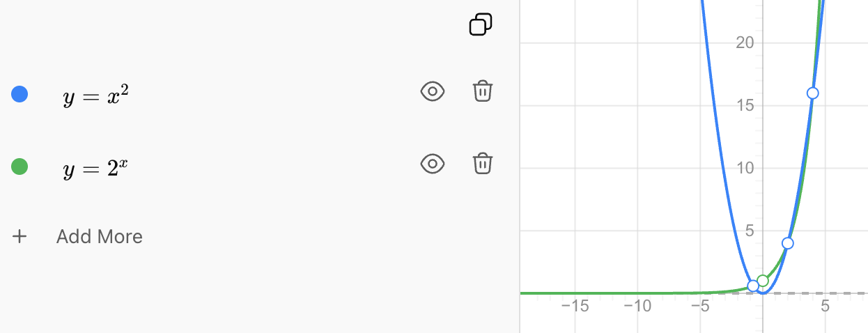
Comparing Quadratic and Exponential Growth
Quadratic and exponential graphs can both curve upward and become increasingly steep.
This means that graph shape alone can sometimes be misleading.
Consider:
Quadratic:
y = x²
Exponential:
y = 2ˣ
For some x-values, the quadratic function may actually be larger.
But exponential growth eventually overtakes polynomial growth such as quadratic growth and then increases much more rapidly.


5. Modeling with Functions
Learning outcomes
- I can choose an appropriate function type.
- I can justify my choice of model.
- I can interpret model predictions.
- I can evaluate limitations of models.
- I can solve practical problems using function models.


