Linear Relationships and Functions

Сайт: Young Education
Курс: Linear Equations and Inequalities
Книга: Linear Relationships and Functions
Надруковано: Guest user
Дата: понеділок 9 листопада 2026 16:38 PM

1. Patterns and Linear Relationships

Learning outcomes
  • I can identify linear patterns in tables and sequences.
  • I can determine the constant rate of change in a pattern.
  • I can extend linear patterns using algebraic rules.
  • I can describe relationships between variables.
  • I can distinguish linear relationships from non-linear relationships.

Patterns and Linear Relationships

A pattern is a repeated or predictable arrangement of numbers, shapes, or quantities. In mathematics, recognizing patterns helps us predict what comes next and describe how quantities are related.

A linear pattern changes by a constant amount.

Consider the sequence:

4, 7, 10, 13, 16, ...

Each term increases by:

+3

Because the same amount is added each time, this is a linear pattern.

Linear patterns are closely connected to linear equations, tables, graphs, and real-world situations involving a constant rate of change.


Recognizing Patterns in Sequences

A sequence is an ordered list of numbers or other mathematical objects.

For example:

5, 9, 13, 17, 21, ...

Look at the difference between consecutive terms:

9 − 5 = 4

13 − 9 = 4

17 − 13 = 4

21 − 17 = 4

The difference is always:

+4

Therefore, the sequence is linear.

The value 4 is called the common difference.


Constant Difference

A numerical sequence is linear when the difference between consecutive terms is constant.

Consider:

20, 17, 14, 11, 8, ...

Differences:

17 − 20 = −3

14 − 17 = −3

11 − 14 = −3

8 − 11 = −3

The common difference is:

−3

This is still a linear pattern.

A linear pattern can increase or decrease.


Increasing Linear Patterns

Consider:

2, 7, 12, 17, 22, ...

The pattern increases by:

5

each time.

The common difference is:

+5

An increasing linear pattern has a positive rate of change.


Decreasing Linear Patterns

Consider:

30, 26, 22, 18, 14, ...

The pattern decreases by:

4

each time.

The common difference is:

−4

A decreasing linear pattern has a negative rate of change.


Constant Patterns

Consider:

8, 8, 8, 8, 8, ...

The difference between consecutive terms is:

0

This is also a linear pattern because its rate of change is constant.

Its constant rate of change is:

0


Patterns in Tables

Linear relationships can also be identified using tables.

Consider:

x y
0 2
1 5
2 8
3 11
4 14

As x increases by 1, y increases by 3.

Therefore:

rate of change = 3

This table represents a linear relationship.

https://images.openai.com/static-rsc-4/lcsqnHo_uhyeX3VLncqdI1qq-amuQ2RXeattwo56iusWY4Iuvmd5_PuAe4OJWptHW12c32EviDf2ReOtfg6dHeg8PUiD_pvrQxlnwyDymVbFk8-lGwLIQ7TheFs9iJ_ZervxW_TwKxIRCYKjsNz-xOPWuoN8xR9lv6PfgzGRLaY5-inLbsgbn7YguuvDPq1Q?purpose=fullsize
 
https://images.openai.com/static-rsc-4/bOHyGrR2RDJzraJFRJFdBtTMcyljFfG_05M8tAI93TjBQc0BX9KAMD6i9-1TBUCIkHgZ42Z5G_2w_gdsbV0jzIeYgI1crBfv2Gzh8JxmIaZ6i_efCa7SVWQ5p471opFrHuXZEWloBtqvAJBUBUjphtyGuoxNfxsnRIGFqAQrzrbQUWdj9ZEXzO3k5kVQUBEX?purpose=fullsize
 
https://images.openai.com/static-rsc-4/GHI0v-m1PD2U96i56OZDUvccjKIeixxSvEIbU87wrph40296hmJfujFMb3pS0tfFcXl9EV9OJL897lF9OQ00bzBu0d6rdtqla-5O0OG0p9plZg4PQRYTAyWDRfm4qfrE7tM8a8sZXsjL6o24z2meugOZcEmwyXF0Bi7w7Z9zSt39cvvhD_bVXFY9GIEuwbam?purpose=fullsize
 
10

Rate of Change

The rate of change describes how much one variable changes compared with another variable.

It can be calculated using:

rate of change = change in y / change in x

or:

rate of change = Δy/Δx

The symbol Δ means "change in."

For example, suppose:

x changes from 2 to 5

and:

y changes from 7 to 19

Then:

Δx = 5 − 2 = 3

Δy = 19 − 7 = 12

Therefore:

rate of change = 12/3

rate of change = 4


Constant Rate of Change

A relationship is linear when its rate of change remains constant.

Consider:

x y
1 7
2 11
3 15
4 19

For every increase of 1 in x:

y increases by 4.

Therefore:

Δy/Δx = 4/1 = 4

The rate of change is constant, so the relationship is linear.


When x Does Not Increase by 1

Do not simply look at the change in y unless the change in x is always 1.

Consider:

x y
0 5
2 11
4 17
6 23

Here:

Δx = 2

and:

Δy = 6

Therefore:

rate of change = 6/2

rate of change = 3

The relationship is linear because this rate remains constant.


Unequal x-Intervals

Consider:

x y
1 5
3 11
7 23
10 32

The x-values do not increase by equal amounts, so calculate the rate carefully.

From the first to second row:

rate = (11 − 5)/(3 − 1)

= 6/2

= 3

From the second to third:

rate = (23 − 11)/(7 − 3)

= 12/4

= 3

From the third to fourth:

rate = (32 − 23)/(10 − 7)

= 9/3

= 3

The rate is always 3.

Therefore, the relationship is linear.


Linear Rules

A linear relationship can often be represented using:

y = mx + b

where:

m = constant rate of change

and:

b = starting value when x = 0

This is called a linear equation.

For example:

y = 3x + 2

has:

rate of change = 3

starting value = 2


Connecting a Table to a Rule

Consider:

x y
0 4
1 7
2 10
3 13
4 16

First identify the rate of change.

Each y-value increases by:

3

Therefore:

m = 3

Now look at the value when x = 0:

y = 4

Therefore:

b = 4

The rule is:

y = 3x + 4


Checking the Rule

For:

y = 3x + 4

when x = 2:

y = 3(2) + 4

y = 6 + 4

y = 10

The table gives y = 10 when x = 2.

Therefore, the rule works.


Extending a Pattern Using a Rule

Suppose:

y = 5x + 2

To determine y when x = 10:

y = 5(10) + 2

y = 50 + 2

y = 52

An algebraic rule allows us to find values far beyond those shown in a table.

We do not need to extend the pattern one step at a time.


Sequences and Term Numbers

Sequences can also be described using algebraic rules.

Consider:

5, 8, 11, 14, 17, ...

Let n represent the term number.

n Term
1 5
2 8
3 11
4 14
5 17

The common difference is:

3

A rule for the sequence is:

T = 3n + 2

where T represents the term value.


Checking a Sequence Rule

For:

T = 3n + 2

find the fourth term.

T = 3(4) + 2

T = 12 + 2

T = 14

This agrees with the sequence.


Finding a Sequence Rule

Consider:

7, 12, 17, 22, 27, ...

The common difference is:

5

Start with:

T = 5n + b

Use the first term:

n = 1

T = 7

Therefore:

7 = 5(1) + b

7 = 5 + b

b = 2

So:

T = 5n + 2


Why the Starting Number Is Not Always b

Consider the sequence:

7, 12, 17, 22, ...

The first term is 7, but the equation is:

T = 5n + 2

not:

T = 5n + 7

This happens because the first term corresponds to:

n = 1

not n = 0.

If we extended the pattern backward to term 0:

2, 7, 12, 17, 22, ...

then the value at n = 0 would be 2.

That is the value of b.


Finding Later Terms Efficiently

Suppose:

T = 4n − 1

Find the 50th term.

Substitute:

n = 50

T = 4(50) − 1

T = 200 − 1

T = 199

An algebraic rule is much faster than writing all 50 terms.


Describing Relationships Between Variables

Variables often represent quantities that change together.

Suppose a taxi charges:

  • $5 starting fee
  • $3 per kilometre

Let:

d = distance travelled in kilometres

C = total cost in dollars

The relationship is:

C = 3d + 5

This tells us:

  • each additional kilometre adds $3
  • the rate of change is $3/km
  • the initial cost is $5
  • cost depends on distance

Independent and Dependent Variables

In many relationships, one variable affects another.

The independent variable is the variable we choose or control.

The dependent variable changes in response.

In:

C = 3d + 5

distance d is the independent variable.

Cost C is the dependent variable.

The cost depends on how far the taxi travels.


Real-World Linear Relationship: Hourly Pay

Suppose a worker earns:

$18 per hour

and receives a fixed:

$25 bonus

Let:

h = hours worked

P = total pay

Then:

P = 18h + 25

The rate of change is:

$18/hour

The starting value is:

$25

https://images.openai.com/static-rsc-4/LUHE6G1IFMlhWM8uyO19wYP36wpidz2YXpIeW1jR_xho3gH8tqIBHqTUC9hRDBBUdXFGhZ6nGrk-KS36aPCbJsV5CasCUECEmU1UxRzz10cFs1FvK7jd4SBfTlLg5oq6QHk6kis05JMnDaRE3SMr1So-E1i8kx-Iyud1LoFvvJ87Fz463bV4F19j8Ool5F8d?purpose=fullsize
 
https://images.openai.com/static-rsc-4/akPZdS47F8NUW_4uZXhKFc74S79d2epy_qFgckkmJuC4nVkuWVUHl7dnHH2CwDhrh3sF10rTf-q_k8OTj1sxV_OMB-nmodmLHht9uThvgAdh6qf3DU6g5FTXYF_UV93a4sEiJtGAeX2aVwD3ggiDgdt_zQRMRvHi9xAYTRPKm7tQ15qDeehs6vmoLsbLPGK1?purpose=fullsize
 
https://images.openai.com/static-rsc-4/W_UU4zE8ly0mippcxnLJCRRKjtO3DWiw3GG_Ty8XZEaueu5pchTjprkZ1UnItlA3khRTbPdmQG__kfGayquo3uinw6ZVnKp51mWv1arXH76Sh3kx9ozrATusay99lJrAdT3d48TMtX7y7tG-Il0tp47_I54dIta-wfd5rVgOwNos0GIQR4BX8hDI2eJLvPG2?purpose=fullsize
 
9

Building a Table from a Rule

For:

P = 18h + 25

we can construct:

Hours h Pay P
0 $25
1 $43
2 $61
3 $79
4 $97

Each additional hour increases pay by:

$18

This constant increase confirms that the relationship is linear.


Linear Relationships and Graphs

When a linear relationship is graphed on a coordinate plane, its points lie on a straight line.

For example:

y = 2x + 1

produces:

x y
0 1
1 3
2 5
3 7
4 9

The y-value increases by 2 whenever x increases by 1.
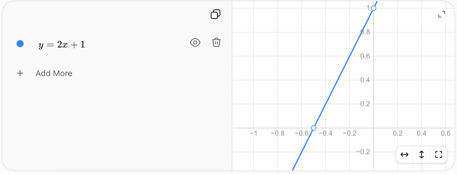
The straight-line graph is another way to recognize a linear relationship.


Rate of Change and Steepness

The rate of change affects how steep a linear graph appears.

Compare:

y = x

and:

y = 4x

The second relationship changes four times as quickly.

A larger positive rate of change produces a steeper upward line.

A negative rate of change produces a line that falls from left to right.


Positive Rate of Change

Consider:

y = 3x + 2

The rate of change is:

3

As x increases, y increases.

The graph rises from left to right.


Negative Rate of Change

Consider:

y = −2x + 10

The rate of change is:

−2

Every time x increases by 1:

y decreases by 2.

For example:

x y
0 10
1 8
2 6
3 4
4 2

The relationship is still linear because the rate of change remains constant.


Zero Rate of Change

Consider:

y = 6

No matter what x is, y remains 6.

Therefore:

rate of change = 0

The graph is a horizontal line.

This is still a linear relationship.


Linear vs Non-Linear Relationships

The defining feature of a linear relationship is a constant rate of change.

Consider:

x y
0 1
1 4
2 7
3 10

Changes in y:

+3, +3, +3

This is linear.

Now consider:

x y
0 1
1 2
2 4
3 8

Changes in y:

+1, +2, +4

The differences are not constant.

This relationship is non-linear.


A Quadratic Pattern

Consider:

1, 4, 9, 16, 25, ...

These are square numbers:

1², 2², 3², 4², 5²

First differences:

3, 5, 7, 9

The first differences are not constant.

Therefore, this sequence is not linear.

It follows a quadratic pattern.


An Exponential Pattern

Consider:

2, 4, 8, 16, 32, ...

Each term is multiplied by:

2

The differences are:

2, 4, 8, 16

They are not constant.

Therefore, this pattern is not linear.

It is an exponential pattern.

A constant multiplication factor does not produce a linear pattern.


Additive vs Multiplicative Patterns

Linear patterns are generally additive.

Example:

3, 8, 13, 18, 23

Add 5 each time.

Exponential patterns are generally multiplicative.

Example:

3, 6, 12, 24, 48

Multiply by 2 each time.

This distinction is useful when identifying patterns.


A Pattern Can Look Regular Without Being Linear

Consider:

1, 4, 9, 16, 25

The sequence clearly follows a pattern.

However, it is not linear.

A pattern is not automatically linear simply because it follows a predictable rule.

To be linear, it must have a constant rate of change.


Using First Differences

One useful way to identify a linear sequence is to calculate first differences.

Consider:

11, 16, 21, 26, 31

First differences:

16 − 11 = 5

21 − 16 = 5

26 − 21 = 5

31 − 26 = 5

Because the first differences are constant:

The sequence is linear.


Non-Linear First Differences

Consider:

2, 5, 10, 17, 26

First differences:

3, 5, 7, 9

Because the first differences change:

The sequence is non-linear.

In later mathematics, patterns in the differences themselves can help identify other types of relationships.


Constant Rate with Different Intervals

A common mistake is to expect equal changes in y when x changes by unequal amounts.

Consider:

Time серце Distance (km)
1 60
2 120
4 240
7 420

The changes in distance are not identical:

+60, +120, +180

But the changes in time are also different:

+1, +2, +3

Calculate the rates:

60/1 = 60

120/2 = 60

180/3 = 60

The rate is always:

60 km/h

Therefore, the relationship is linear.


Distance and Constant Speed

If an object travels at constant speed:

distance = speed × time

Suppose a cyclist travels at:

15 km/h

Then:

d = 15t

where:

d = distance in kilometres

t = time in hours

The constant rate of change is:

15 km/h

This is a linear relationship.


Starting Values in Real Situations

Not every linear relationship begins at zero.

Suppose a water tank initially contains:

100 L

and fills at:

8 L/min

Let:

t = time in minutes

V = volume in litres

Then:

V = 8t + 100

The rate of change is:

8 L/min

The starting value is:

100 L

At t = 0:

V = 100


Decreasing Real-World Pattern

Suppose a tank contains:

500 L

and loses water at:

20 L/min

The relationship is:

V = 500 − 20t

or:

V = −20t + 500

The rate of change is:

−20 L/min

The negative rate tells us that the amount of water decreases over time.


Extending a Table

Suppose:

x y
1 9
2 14
3 19
4 24

The constant difference is:

+5

Continue the pattern:

x y
5 29
6 34
7 39

The rule is:

y = 5x + 4

Using the rule, we can calculate any value directly.


Predicting Far Beyond a Table

Using:

y = 5x + 4

find y when:

x = 100

Substitute:

y = 5(100) + 4

y = 500 + 4

y = 504

This is one of the major advantages of algebraic rules: they allow us to make predictions without extending a table one row at a time.


Working Backward

An algebraic rule can also be used to determine an input from an output.

Suppose:

y = 4x + 3

and:

y = 35

Then:

35 = 4x + 3

Subtract 3:

32 = 4x

Divide by 4:

x = 8

This tells us that 35 occurs when x = 8.


Comparing Two Linear Patterns

Consider:

Pattern A:

y = 2x + 5

Pattern B:

y = 4x + 1

Pattern A has:

rate of change = 2

Pattern B has:

rate of change = 4

Therefore, Pattern B grows more quickly.

However, Pattern A begins with a larger starting value.

This means one pattern may begin larger even though the other eventually overtakes it.


Finding Where Two Patterns Are Equal

Using:

y = 2x + 5

and:

y = 4x + 1

set the expressions equal:

2x + 5 = 4x + 1

Subtract 2x:

5 = 2x + 1

Subtract 1:

4 = 2x

x = 2

At x = 2:

Pattern A:

2(2) + 5 = 9

Pattern B:

4(2) + 1 = 9

The two patterns meet at:

(2, 9)


Comparing Linear Relationships from Tables

Suppose:

Pattern A

x y
0 5
1 8
2 11
3 14

Rate:

3

Now consider:

Pattern B

x y
0 1
1 6
2 11
3 16

Rate:

5

Pattern B changes more quickly because:

5 > 3

Even though Pattern A begins with a larger value.


Connecting Tables, Rules, and Graphs

A linear relationship can be represented in several ways.

Words

"Start at 4 and increase by 3 each time."

Table

x y
0 4
1 7
2 10

Rule

y = 3x + 4

Graph

A straight line with a constant rate of change of 3.

These are different representations of the same relationship.

https://images.openai.com/static-rsc-4/JK7b8ZM_rwMZiXDFwwxtTRFC6wrwoYXJacEaBWrL9xr2ZXDvDleb9gcqNzBdVikh7Aa-pfKkaDuvOoIDyMrtQytXRfnSdno_d8FW4d0R0M1bd9X3uZYLf0TBE4hvT4gyRrp7lh4rzNpeqEN0m2jD48zhshS6Qv6q0G4I37BQz8chaxo1rZSprNT8YXSjYADd?purpose=fullsize
 
https://images.openai.com/static-rsc-4/yl947in3Ufe77JB5Gf0O0DIkF_-yc9y6yj-TwWcJq1ukZgOj6XUELz26NxnwKZU7nk12h9eRDAFSXenHxLX5o9p4ibSFKuwoqZkA0HVytRAUwjGAmzybtztQEIKIW0oKysV1cQ_VXINWJd0yO6fCaR-c3al-YRkPKsuMAx4ovZD_fC8VeNwvtlUlNUOcRdM0?purpose=fullsize
 
https://images.openai.com/static-rsc-4/rw8_DONyrXhVQWyXpk70t2Os-GmJlWxDNyUXhSFFsjJ8wjUdONNxleF5AxLBe9q_DkM9eiw2v1p-idlgMz-yMkq2u3xEZb0znQQ6Nkd8FRSP2v0tM_XBqOcPqulFjLazGk8EaOHRS99pfH7yXLslv3wsHu8fYJwYfdO7_PnHHDfGvW2wQWcRBckT_c2JcHOu?purpose=fullsize
 
9

Interpreting the Rate in Context

The rate of change should always include meaning and units.

If:

C = 4d + 6

where C is taxi cost in dollars and d is distance in kilometres:

rate = $4/km

This means:

The cost increases by $4 for every additional kilometre travelled.

Simply saying "the rate is 4" is mathematically incomplete when interpreting a real situation.


Interpreting the Starting Value

For:

C = 4d + 6

the starting value is:

6

In context:

The taxi costs $6 before any distance is travelled.

The starting value might represent:

  • an initial fee
  • an initial population
  • starting height
  • initial volume
  • starting balance
  • initial temperature

Its meaning depends on the situation.


Practical Example: Phone Plan

A phone plan costs:

$25 per month

plus:

$3 per GB of additional data

Let:

g = additional data in GB

C = total cost

Then:

C = 3g + 25

The rate of change is:

$3/GB

The starting value is:

$25

If 8 GB of additional data is used:

C = 3(8) + 25

C = 24 + 25

C = $49


Practical Example: Saving Money

Suppose you already have:

$120

and save:

$25 each week

Let:

w = number of weeks

S = total savings

Then:

S = 25w + 120

After 10 weeks:

S = 25(10) + 120

S = 250 + 120

S = $370

This is linear because the savings increase by the same amount each week.


Practical Example: Candle Burning

A candle begins at:

30 cm

and burns down at:

2 cm per hour

Let:

t = time in hours

h = candle height

Then:

h = 30 − 2t

The rate of change is:

−2 cm/h

The negative sign indicates that the candle becomes shorter.

After 6 hours:

h = 30 − 2(6)

h = 18

The candle is:

18 cm tall

under this model.


When a Linear Model Stops Making Sense

The candle equation:

h = 30 − 2t

is mathematically defined for many values of t.

But eventually it predicts negative candle heights.

For example:

t = 20

h = 30 − 40

h = −10 cm

A candle cannot have a physical height of −10 cm.

Therefore, the mathematical model only makes sense over a limited domain.

This is an important part of interpreting real-world linear relationships.


Linear Patterns in Geometry

Suppose a row of connected squares is built with matchsticks.

If each new square shares one side with the previous square, each additional square adds a constant number of matchsticks.

A possible pattern is:

4, 7, 10, 13, 16, ...

The common difference is:

3

Therefore, the pattern is linear.

https://images.openai.com/static-rsc-4/oy_EeOVY7jEtzOytVN4hqQzyOEvDqUoI8aRfMMWd6U1r39cTvMn2vgWKvFygirPDOI4q3eaJ6QLhkhUYZdHUZcsdNg2Tb5ioa7jo9Rb97NEFDK-py_YUWk4qJvrnTf6WgtrcmWlCfCGRwnq9kvInYTI3Gq2O5ZGgBMZml4O4btJYEYEyiLpI-RuqvSnjNHEN?purpose=fullsize
 

Finding the Rule for a Geometric Pattern

Suppose:

Number of Squares n Matchsticks M
1 4
2 7
3 10
4 13

The rate is:

3 matchsticks per additional square

Use:

M = 3n + b

Substitute n = 1 and M = 4:

4 = 3(1) + b

b = 1

Therefore:

M = 3n + 1

For 20 squares:

M = 3(20) + 1

M = 61


Identifying Linear Relationships Quickly

Ask these questions:

From a sequence:
Are the first differences constant?

From a table:
Is Δy/Δx constant?

From an equation:
Can it be written in the form y = mx + b?

From a graph:
Do the points form a straight line?

From a situation:
Does one quantity change by a constant amount for each unit change in another quantity?

If yes, the relationship is likely linear.


Identifying Non-Linear Relationships

A relationship is non-linear if its rate of change is not constant.

Common examples include:

Quadratic

y = x²

Exponential

y = 2ˣ

Inverse

y = 1/x

These relationships do not form straight lines and do not have a constant rate of change over their entire domains.


Linear or Non-Linear?

Consider:

Pattern A

2, 6, 10, 14, 18

Differences:

+4, +4, +4, +4

Linear

Consider:

Pattern B

2, 6, 18, 54, 162

Each term is multiplied by 3.

Differences are not constant.

Non-linear

Consider:

Pattern C

3, 3, 3, 3, 3

Differences:

0, 0, 0, 0

Linear


A Reliable Strategy for Analyzing Patterns

When given a sequence, table, graph, or situation:

  1. Identify the variables or term numbers.
  2. Calculate changes in the input.
  3. Calculate changes in the output.
  4. Determine Δy/Δx.
  5. Check whether the rate remains constant.
  6. If constant, identify the relationship as linear.
  7. Determine the rate of change.
  8. Find the starting value.
  9. Write an algebraic rule if possible.
  10. Use the rule to extend or predict values.
  11. Interpret the rate and starting value in context.
  12. Check whether the model remains realistic for the values being considered.

Common Mistakes

Looking only for a pattern

A predictable pattern is not necessarily linear. Linear patterns specifically require a constant rate of change.

Checking y-values without considering x-values

If x changes by different amounts, calculate:

Δy/Δx

rather than only comparing y-differences.

Thinking decreasing patterns are non-linear

A constant negative rate of change is still linear.

Thinking a constant pattern is non-linear

A constant rate of zero is linear.

Confusing additive and multiplicative patterns

Adding the same amount produces a linear sequence. Multiplying by the same factor usually produces an exponential pattern.

Using the first term as b

In a sequence where n starts at 1, the first term is not necessarily the value of b.

Ignoring units

A rate should be interpreted using units such as dollars/hour, kilometres/hour, or litres/minute.

Assuming every algebraic pattern is linear

Equations containing x², x³, √x, 1/x, or similar expressions are generally non-linear.

Extending a real-world model beyond a reasonable domain

A linear rule may be mathematically valid for values that make no physical sense.


Key Terms

Pattern — predictable arrangement or change in numbers, shapes, or quantities.

Sequence — ordered list of numbers or mathematical objects.

Term — individual value in a sequence.

Term number — position of a term within a sequence.

Linear pattern — pattern with a constant rate of change.

Non-linear pattern — pattern whose rate of change is not constant.

Common difference — constant difference between consecutive terms of a linear sequence.

First differences — differences between consecutive terms in a sequence.

Rate of change — amount one variable changes relative to another.

Constant rate of change — rate that remains the same throughout a relationship.

Independent variable — variable used as the input or controlled quantity.

Dependent variable — variable whose value depends on another variable.

Linear relationship — relationship between variables having a constant rate of change.

Linear equation — equation representing a linear relationship, commonly written y = mx + b.

Starting value — value of the dependent variable when the independent variable is zero.

Algebraic rule — equation describing how variables or pattern values are related.

Domain — set of input values for which a relationship or model is defined or meaningful.

Prediction — value estimated or calculated from an identified relationship.


Key Takeaways

  • Patterns can be represented using sequences, tables, equations, graphs, and words.
  • A linear pattern has a constant rate of change.
  • In a sequence with consecutive term numbers, a constant first difference indicates a linear pattern.
  • Linear patterns may increase, decrease, or remain constant.
  • A positive rate produces an increasing relationship.
  • A negative rate produces a decreasing relationship.
  • A zero rate produces a constant relationship.
  • Rate of change can be calculated using Δy/Δx.
  • When x-values have unequal intervals, both Δx and Δy must be considered.
  • Linear relationships can often be written as y = mx + b.
  • In y = mx + b, m represents the rate of change and b represents the starting value.
  • An algebraic rule can extend a pattern far beyond the values shown in a table.
  • Linear graphs form straight lines.
  • A predictable pattern is not necessarily linear.
  • Quadratic and exponential patterns are examples of non-linear relationships.
  • Repeated addition or subtraction commonly indicates a linear pattern.
  • Repeated multiplication usually indicates a non-linear pattern.
  • Rates should be interpreted with appropriate units.
  • Real-world linear models may only make sense over a restricted domain.
  • Tables, equations, graphs, and verbal descriptions can all represent the same linear relationship.

Check Your Understanding

  1. Determine whether 4, 9, 14, 19, 24, ... is a linear sequence. If it is, state the common difference.
  2. Determine whether 3, 6, 12, 24, 48, ... is linear. Explain your reasoning.
  3. Find the next three terms in 30, 26, 22, 18, ....
  4. Determine the constant rate of change in the table:
x y
0 6
1 10
2 14
3 18
  1. Determine whether the relationship is linear:
x y
0 2
2 8
5 17
9 29

Show how you calculated the rates.

  1. Write an algebraic rule for the sequence 6, 10, 14, 18, 22, ..., where n = 1 represents the first term.
  2. Use your rule from Question 6 to determine the 50th term.
  3. A relationship has a rate of change of −3 and a starting value of 20. Write an equation in the form y = mx + b.
  4. A taxi charges a starting fee of $7 plus $4 per kilometre. Define variables and write a linear equation relating cost and distance. Explain the meaning of the rate of change.
  5. A tank initially contains 350 L and loses 15 L each minute. Write a linear equation for its volume after t minutes. Determine its volume after 12 minutes.
  6. Compare y = 3x + 8 and y = 5x + 2. Which has the greater rate of change? Which has the greater starting value?
  7. Determine whether 2, 5, 10, 17, 26, ... is linear. Use first differences to justify your answer.
  8. A student says that 5, 10, 20, 40, 80, ... is linear because there is a clear pattern. Explain the student's mistake and identify what type of change is occurring.
  9. A worker begins with a $40 bonus and earns $22 per hour. Create a table for 0 through 5 hours, write the algebraic rule, identify the independent and dependent variables, and explain the meaning of both the rate of change and starting value.
  10. A candle begins at 36 cm tall and burns down at a constant rate of 3 cm per hour. Write a linear equation for its height, determine when the candle reaches 12 cm, and explain why the same linear model should not be used indefinitely.


2. Functions and Function Notation

Learning outcomes
  • I can define a function as a relationship between inputs and outputs.
  • I can identify whether a relation is a function.
  • I can evaluate functions using function notation.
  • I can interpret function values in context.
  • I can represent functions using tables, graphs, and equations.

Functions and Function Notation

A function is a relationship between inputs and outputs in which each input has exactly one output.

Think of a function as a machine:

input → function rule → output

For example, suppose the rule is:

y = 2x + 3

If the input is x = 4:

y = 2(4) + 3

y = 11

So:

input 4 → output 11

The most important rule is:

One input cannot produce two different outputs if the relationship is a function.


Inputs and Outputs

A function connects two quantities.

The input is the value entered into the function.

The output is the value produced.

For:

y = 3x + 5

x is the input.

y is the output.

If x = 2:

y = 3(2) + 5

y = 11

Therefore:

2 → 11


Independent and Dependent Variables

The input is often called the independent variable.

The output is often called the dependent variable because its value depends on the input.

Consider:

C = 4h + 10

where:

h = hours

C = cost

The number of hours is the input.

The cost is the output.

Changing h causes C to change.


What Makes a Relation a Function?

A relation is any collection of input-output pairs.

For example:

(1, 5), (2, 7), (3, 9), (4, 11)

Each input appears with exactly one output.

Therefore, this relation is a function.

Now consider:

(1, 5), (2, 7), (2, 10), (3, 12)

Input 2 has two outputs:

2 → 7

and:

2 → 10

Therefore, this relation is not a function.


Repeated Outputs Are Allowed

A common misunderstanding is that outputs cannot repeat.

They can.

Consider:

(1, 5), (2, 5), (3, 7), (4, 7)

Different inputs produce the same outputs.

That is allowed.

Each input still has only one output.

Therefore:

This relation is a function.

The rule applies to repeated inputs, not repeated outputs.


Repeated Inputs

Consider:

(1, 4), (2, 6), (2, 6), (3, 8)

The repeated input 2 still produces the same output, 6.

This does not create two different outputs.

The relationship can still represent a function.

The problem occurs when one input is connected to different outputs.


Functions in Tables

Consider:

Input x Output y
1 4
2 7
3 10
4 13

Every input has exactly one output.

Therefore, the table represents a function.


A Table That Is Not a Function

Consider:

Input x Output y
1 5
2 8
2 11
3 14

Input 2 produces:

8 and 11.

Therefore:

This relation is not a function.


Mapping Diagrams

Functions can also be represented using mapping diagrams.

A mapping diagram shows arrows connecting inputs to outputs.

For example:

1 → 4
2 → 6
3 → 8
4 → 10

Every input has one arrow leading to one output.

Therefore, the relation is a function.

https://images.openai.com/static-rsc-4/DIWXHN8Fz4y1UIzieCeMilpGOU88TQpx3-L7S9P-Avcu0l8EW5b-G1rlUsBptvCIMx29R2_p2XVq6t78hRf8Rnj64Syu926Gcx6mMyRfgnvso7POizfjqRuki-1lG3XifItdtAIQJ6nRPWHkjH3m0iK6B_d_iUIUWDmd9ALl09rzcVSXBRsnNhAyotq87LOx?purpose=fullsize
 
https://images.openai.com/static-rsc-4/D2cCE461mfOwdIpHd7CpZldtcGd51ZJyMbEyLeLibAexkclZ7n8u5EKvWpGfUxsrt03r6xuYqfC-HT_f_u0MjFup8pNJsbaHPnrkjKfFm7DoUg4f7NtVuBf3JX6rtl6zUl7OXXeBJCpLwCEuJZkEgWzJqTu8OQg7Qu0tCpaLCNgBVDSDK8AW3VfwyD3vAYXZ?purpose=fullsize
 
https://images.openai.com/static-rsc-4/5eGqqvnt6Yf8TSte8CaAtBcPCyts8i1ln4QGu6EnqlCNOzWg7oNPER9wK9i3pZY6-YtU1osbAXz5aICCU53BeNZNWclSUgoTBhLKRfGrLUh5k17UzEb2I37bhdje5htff8YHLfF4qnPbgvJ6VHV4hOe5EUuej2y67y3W6ognp3G-B4MeQZZD6JlPbb9-7gLd?purpose=fullsize
 
7

Identifying Functions from Mapping Diagrams

Suppose:

1 → 5
2 → 6
3 → 6
4 → 8

This is a function.

Although inputs 2 and 3 share the same output, each input still has only one output.

Now suppose:

1 → 5
2 → 6
2 → 9
3 → 10

This is not a function because input 2 produces two different outputs.


Function Notation

Instead of writing:

y = 2x + 3

we can write:

f(x) = 2x + 3

This is called function notation.

The expression:

f(x)

is read:

"f of x"

It does not mean:

f × x

Instead, f(x) represents the output of function f when the input is x.


Understanding f(x)

If:

f(x) = 3x + 4

then:

f(2)

means:

the output when the input is 2

Substitute 2 for x:

f(2) = 3(2) + 4

f(2) = 6 + 4

f(2) = 10


Evaluating a Function

Suppose:

f(x) = 5x − 2

Find:

f(4)

Replace every x with 4:

f(4) = 5(4) − 2

f(4) = 20 − 2

f(4) = 18

Therefore, input 4 produces output 18.


Evaluating a Function at Zero

Suppose:

f(x) = 4x + 7

Find:

f(0)

Substitute 0:

f(0) = 4(0) + 7

f(0) = 7

For a linear function, f(0) often represents the starting value.


Evaluating Functions at Negative Values

Suppose:

f(x) = 3x + 8

Find:

f(−2)

Substitute −2:

f(−2) = 3(−2) + 8

f(−2) = −6 + 8

f(−2) = 2

Use parentheses around negative inputs to reduce sign errors.


Evaluating Functions with Exponents

Functions do not have to be linear.

Suppose:

g(x) = x² + 2

Find:

g(3)

g(3) = 3² + 2

g(3) = 9 + 2

g(3) = 11

Now find:

g(−3)

g(−3) = (−3)² + 2

g(−3) = 9 + 2

g(−3) = 11

Different inputs can produce the same output and the relation can still be a function.


Why Parentheses Matter

Suppose:

f(x) = x² − 4x

Find:

f(−2)

Substitute carefully:

f(−2) = (−2)² − 4(−2)

f(−2) = 4 + 8

f(−2) = 12

Writing negative inputs inside parentheses helps preserve the correct signs.


Evaluating Decimal Inputs

Suppose:

f(x) = 2x + 5

Find:

f(1.5)

f(1.5) = 2(1.5) + 5

f(1.5) = 3 + 5

f(1.5) = 8

Function inputs do not have to be whole numbers unless the context restricts them.


Evaluating Fraction Inputs

Suppose:

f(x) = 6x + 1

Find:

f(1/2)

f(1/2) = 6(1/2) + 1

f(1/2) = 3 + 1

f(1/2) = 4


Functions as Machines

A useful mental model is a function machine.

For:

f(x) = 2x + 1

the machine:

  1. takes an input
  2. multiplies it by 2
  3. adds 1
  4. produces an output

For example:

3 → multiply by 2 → 6 → add 1 → 7

Therefore:

f(3) = 7

https://images.openai.com/static-rsc-4/-HbRQFtUz57OaAfX3v7aJoMNRECIQKlQ3HWlhXVF_GjU_T_ng1XKXKqZM5PYBNARgejFn3S3sTsdvxX__2iWDoBWKZO7crRkr0obUxOTBRcPjCVbqFXzQ4kg-CzzXQRO5ZH6xFWH8e-JRxzNZycMj6gJd6J29hmOOuuzfZg5LPN_6UGMHp2ZLy14_cnozv7D?purpose=fullsize
 
https://images.openai.com/static-rsc-4/slJmBFJ9T6xPiZEDAaZLcr7Iae8fzz0sabV0mJcAZrRyktSIpNs2laPhH2-HWcX2_krjk6KvbwbooDJw3vu6hj2jZxylIyqb0-xIph_k75ko99ccZU7bXCIV-JXIqzgjYc-tOERLVrqhP59GHbRZ95plUU91OjYqpprG86aqR4F9NM1EDv9sxEN0FwHXhekX?purpose=fullsize
 
https://images.openai.com/static-rsc-4/TchFi7MNSXGxfOD3sboYUkca0bVpN0Bf4i0NzVDdvcQjhy83adOoNzPw6kirpS4l6ouksVKm_6z9fY3ayp8hILBJI2_SrX40CHemO42RQ22st57YVrm1qIFCPdHWP-YK717IPURHQ9RvmQCjOggU9-Hu2wInkLjTMPsIjFxgeyb7aUFAUeLUbVuCZUt21yXx?purpose=fullsize
 
10

Building a Function Table

Suppose:

f(x) = 2x + 3

We can evaluate several inputs.

x f(x)
−2 −1
−1 1
0 3
1 5
2 7

The table represents the same function as the equation.


Moving from a Table to an Equation

Consider:

x f(x)
0 4
1 7
2 10
3 13

The output increases by:

3

for every increase of 1 in x.

Therefore, the rate of change is:

3

At x = 0:

f(0) = 4

So the function rule is:

f(x) = 3x + 4


Function Values from Tables

Suppose:

x f(x)
−2 7
−1 4
0 1
1 −2
2 −5

To find:

f(1)

look for the row where x = 1.

The output is:

−2

Therefore:

f(1) = −2


Finding an Input from a Function Table

Using the same table, suppose we ask:

For what value of x is f(x) = 7?

Find 7 in the output column.

It corresponds to:

x = −2

This is different from being asked to find f(−2).

Function notation requires careful reading.


Evaluating Functions from Graphs

A graph can also represent a function.

To find:

f(2)

from a graph:

  1. locate x = 2 on the horizontal axis
  2. move vertically until you reach the graph
  3. read the corresponding y-value

That y-value is:

f(2)

https://images.openai.com/static-rsc-4/ghErpnYGR-KfScu9QM96RpU1SP5X3_TPtwvZCa0yBUfavFqzW3_JyeGFBLmSPKsL2FjXA-OSZnYtOsM935sdI2lr1iv1MaewqCdSiGSkHTTivrsIwdfjxJ0vbc-j90AcOfgGJ363eYnbUpgkrIe8S2Mbh7jYltsINrjBVmgLypP5CDzV0_YnnC542Vl1GGjQ?purpose=fullsize
 
https://images.openai.com/static-rsc-4/jSByijKNaQCSHBMQPwFN6f5aj3caAIyM4Nm5vxUsltCSYF9YbRtFXqQgF12FBNI5MKZji8ItwQJn9YHfGg_dy-NBkMI9LE-vADk5nczuja_Jrsh81pZq-3SmqJI4Pyvey9o2q7lonmhInqs6Ag1vB9shUiWtiSyTIS0tTZuWaeJlrS-f4yQkoKtlt0F-bsEi?purpose=fullsize
 
https://images.openai.com/static-rsc-4/DD7CwW2qDn3RqWEZFdqhe6LT6cteKuPDiQdq2Qwnsiycn2m6aUostWOVdD0qnlnQ0nWZ6SCiZu66B8dOyeVkirdDGL1sYPZlKc00Y9a7eBPaavo-14kfiFiw99Y1BsPP6jLUktO11JmL2L002V4ACVVszH3wHhPwu-eP6NOS4kq-BpZKj_P_chFJdH_Bwz43?purpose=fullsize
 
10

A Function Graph

Consider:

f(x) = 2x + 1

The graph represents every input-output pair satisfying the function.

For example:

f(0) = 1

f(1) = 3

f(2) = 5

f(3) = 7
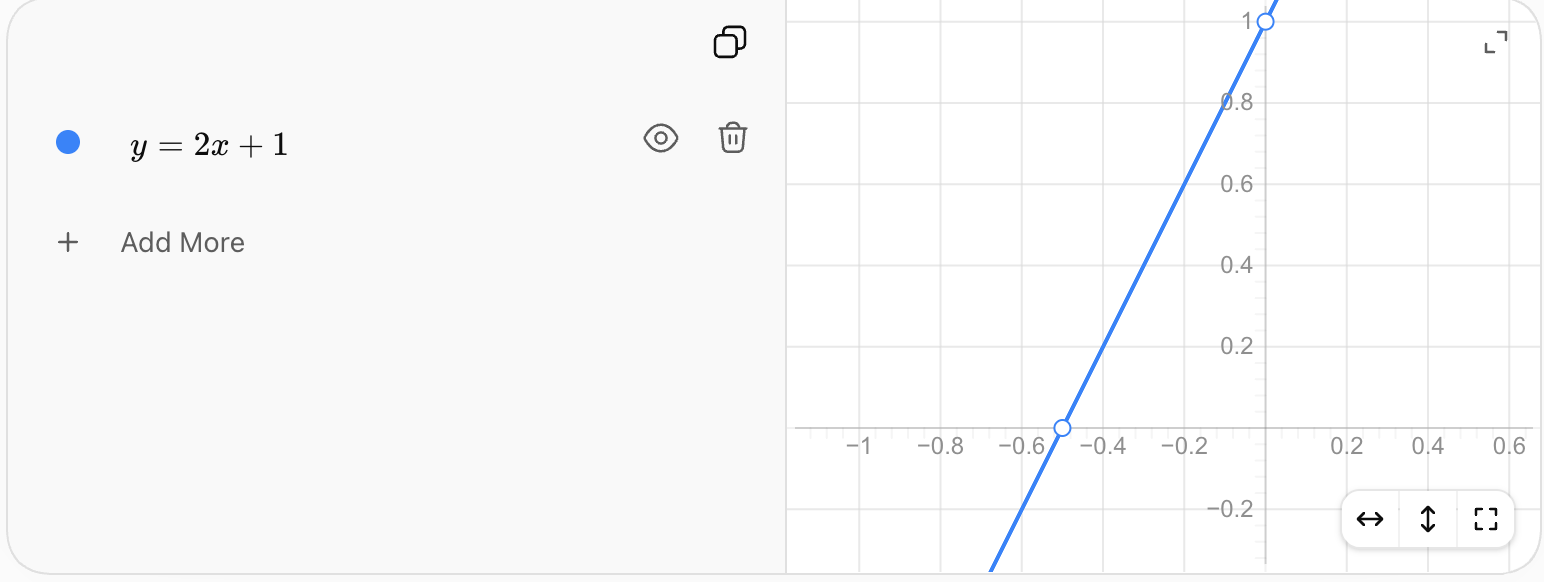
Each x-coordinate has exactly one corresponding y-coordinate.


The Vertical Line Test

A graph represents a function if every input x has no more than one output y.

The vertical line test provides a quick graphical method.

Imagine drawing vertical lines through the graph.

If any vertical line intersects the graph more than once:

the graph is not a function.

If every vertical line intersects at most once:

the graph is a function.


Why the Vertical Line Test Works

A vertical line represents one particular x-value.

If it crosses the graph twice, that same x-value has two different y-values.

That violates the definition of a function.

Therefore:

More than one intersection with a vertical line → not a function.


Function vs Non-Function Graphs

A typical straight line such as:

y = 2x + 3

is a function.

A parabola such as:

y = x²

is also a function.

For each x-value, there is exactly one y-value.

A circle such as:

x² + y² = 25

is not y as a function of x over the entire circle because many x-values correspond to two y-values.

https://images.openai.com/static-rsc-4/mpIlIrT30apulmFI-w7ktu5t0RX7XTKh_3Yjv9P1PEYIoorfoI9e5lSw1CHvoHRYULLermDQ7--EV_y1iv7Wcts0W8qaHhkmUoFg543U58lbVP_xm41vqNfZRZhmQ3ALM_KL6J_y4zK652gpZz5y5oFfFNBrFQcIstNNBFKkHrwbCqM4uSB_L5IaYvlg3rhG?purpose=fullsize
 
https://images.openai.com/static-rsc-4/LOPs_Zh1oA7swmqqnJDtqlU9xizyddvBGhhKGSB6kqxuNQSt6RK1wIT6TwSfHh7Srmd5vnVnbl9FJEYLD0jxCvm82zQm8DGGRbzay4MkmUmRXHqi3FZrswk36GJfuRJ51lAGo68AzY7ja2Vh_QXwvLnWBAn2--X-8WSexA_kicmz6Ys40kLTN0hK0VPOFDbm?purpose=fullsize
 
https://images.openai.com/static-rsc-4/JE11liGbMNXYMEyjZ6iKcBtiJ8VEi_NBDN5EMCmwRuG1lpLVX2TZBXhdKIwoMPX_9ZuJfrRhU4K347NcNDyMPmDl3-0ZI69Te7LzDlNFFwSlv2RbKy8klSaWl2M5UptC3BsR8TT1R0sSHV3FF4CGRt_ts4vrAQftZ7fjrHiIct7eKYg7N9-MhWOB5nNm3gvZ?purpose=fullsize
 
6

A Non-Linear Function

A function does not need to be linear.

For example:

f(x) = x²

is a function.

Its graph is curved rather than straight.
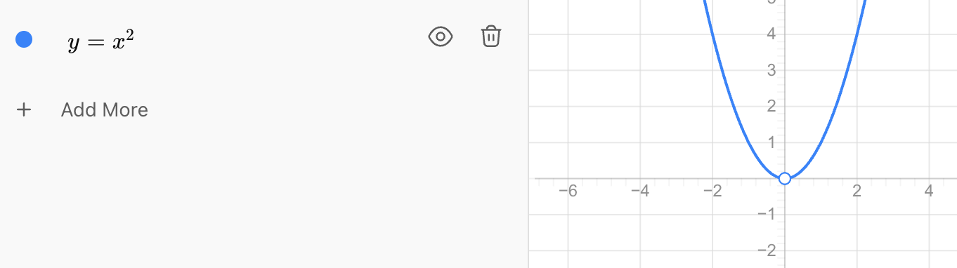
For every input x, there is exactly one output.

For example:

f(2) = 4

and:

f(−2) = 4

Two inputs producing the same output is allowed.


Relations That Are Not Functions

Consider:

x² + y² = 9

This represents a circle.

For x = 0:

y could be:

3

or:

−3

Therefore, the same input x = 0 has two outputs.

So the complete circle is not a function of x.


Domain

The domain is the set of allowed input values.

For example, suppose a function is represented by:

(1, 5), (2, 7), (3, 9), (4, 11)

The domain is:

{1, 2, 3, 4}

These are all the input values.


Range

The range is the set of output values.

For:

(1, 5), (2, 7), (3, 9), (4, 11)

the range is:

{5, 7, 9, 11}

So:

domain = inputs

range = outputs


Repeated Values in the Range

Consider:

(1, 4), (2, 6), (3, 6), (4, 8)

Domain:

{1, 2, 3, 4}

Range:

{4, 6, 8}

The number 6 only needs to be listed once in the range because a set does not repeat elements.


Domain Restrictions

Not every function allows every possible input.

Consider:

f(x) = 10/x

The input:

x = 0

is not allowed because division by zero is undefined.

Therefore, the domain excludes 0.

Domain:

all real numbers except 0


Domain in Real-World Situations

Suppose:

CНі = 8n + 20

represents the cost of ordering n pizzas.

Mathematically, the equation could accept values such as:

n = −4

or:

n = 2.5

But these values do not make sense if n represents a number of pizzas.

The realistic domain might be:

n = 0, 1, 2, 3, ...

Context determines which inputs are meaningful.


Function Notation in Context

Suppose:

CНі = 12n + 5

represents the total cost of ordering n items.

Then:

C(4)

does not simply mean "C times 4."

It means:

the total cost when 4 items are ordered.

Calculate:

C(4) = 12(4) + 5

C(4) = 53

Therefore:

C(4) = $53


Interpreting Function Values

Suppose:

H(t) = 120 − 5t

represents the height of water in a tank, in centimetres, after t minutes.

Then:

H(6)

means:

the height of the water after 6 minutes.

Calculate:

H(6) = 120 − 5(6)

H(6) = 90

Therefore:

After 6 minutes, the water is 90 cm high.

A complete interpretation includes both the value and its meaning.


Units Matter

Suppose:

d(t) = 60t

where:

d = distance in kilometres

t = time in hours

Then:

d(3) = 60(3)

d(3) = 180

A complete interpretation is:

After 3 hours, the object has travelled 180 km.

Not simply:

"d(3) = 180."


Real-World Function: Taxi Cost

Suppose a taxi charges:

  • $6 starting fee
  • $3 per kilometre

Let:

C(d) = 3d + 6

where d is distance in kilometres.

Find:

C(10)

C(10) = 3(10) + 6

C(10) = 36

Therefore:

A 10 km trip costs $36.


Real-World Function: Temperature

Suppose:

Tсерце = 18 + 2h

models temperature in °C, h hours after a measurement begins.

Find:

T(4)

T(4) = 18 + 2(4)

T(4) = 26

Therefore:

The model predicts a temperature of 26°C after 4 hours.


Real-World Function: Falling Water Level

Suppose:

W(t) = 250 − 12t

where W is water volume in litres and t is time in minutes.

Find:

W(5)

W(5) = 250 − 12(5)

W(5) = 190

Therefore:

After 5 minutes, 190 L of water remain.


Different Names for Functions

Functions do not always use the letter f.

We might have:

f(x) = 2x + 1

g(x) = x²

h(t) = 5t − 3

CНі = 12n + 20

T(t) = 25 − 0.5t

The function name can help communicate what the function represents.

For example:

C might represent cost.

T might represent temperature.

P might represent population.


Comparing Two Functions

Suppose:

f(x) = 2x + 5

and:

g(x) = 4x − 1

Find f(3):

f(3) = 2(3) + 5

f(3) = 11

Find g(3):

g(3) = 4(3) − 1

g(3) = 11

At x = 3, both functions have the same output.


Functions Can Be Represented in Different Ways

A function can be represented using:

  • words
  • ordered pairs
  • mapping diagrams
  • tables
  • equations
  • function notation
  • graphs

For example:

Words: Start at 2 and increase by 3 for every unit increase in x.

Equation: y = 3x + 2

Function notation: f(x) = 3x + 2

Table:

x f(x)
0 2
1 5
2 8
3 11

All these representations describe the same relationship.


Moving Between Representations

Suppose a table shows:

x f(x)
0 5
1 9
2 13
3 17

The outputs increase by 4.

Therefore:

rate of change = 4

At x = 0:

f(0) = 5

So:

f(x) = 4x + 5

The table and equation represent the same function.


Functions and Linear Relationships

A linear function can usually be written:

f(x) = mx + b

where:

m = constant rate of change

b = starting value

For example:

f(x) = −3x + 10

has:

rate of change = −3

starting value = 10

Every input still has exactly one output, so it is a function.


Functions Do Not Have to Be Linear

Examples of functions include:

Linear:
f(x) = 2x + 3

Quadratic:
f(x) = x²

Exponential:
f(x) = 2ˣ

Constant:
f(x) = 7

All satisfy the fundamental requirement:

each allowed input produces exactly one output.


Finding an Input When the Output Is Known

Suppose:

f(x) = 3x + 5

and:

f(x) = 20

We want to find the input that produces 20.

Write:

3x + 5 = 20

Subtract 5:

3x = 15

Divide by 3:

x = 5

Therefore:

f(5) = 20


Input vs Output Questions

These two questions are different:

Find f(5).

This gives you the input and asks for the output.

But:

Find x when f(x) = 5.

This gives you the output and asks for the input.

Carefully identify which quantity is known before calculating.


Evaluating an Expression as an Input

Function notation can contain expressions rather than just numbers.

Suppose:

f(x) = 2x + 3

Find:

f(a)

Replace x with a:

f(a) = 2a + 3

Now find:

f(a + 1)

Replace every x with:

a + 1

f(a + 1) = 2(a + 1) + 3

f(a + 1) = 2a + 2 + 3

f(a + 1) = 2a + 5

This idea becomes important in more advanced algebra.


A Function as a Rule

A function can be thought of as a rule assigning each allowed input exactly one output.

For:

f(x) = x² − 1

the rule says:

  1. take the input
  2. square it
  3. subtract 1

For x = 4:

f(4) = 4² − 1

f(4) = 16 − 1

f(4) = 15

The same rule is applied consistently to every allowed input.


Evaluating Functions Efficiently

When evaluating a function:

  1. Write the function.
  2. Identify the requested input.
  3. Replace every occurrence of the variable with the input.
  4. Use parentheses when substituting negative numbers or expressions.
  5. Follow the order of operations.
  6. Simplify.
  7. Include units and interpretation when working in context.

Determining Whether a Relation Is a Function

When given a relation, ask:

Ordered pairs:
Does any input have two different outputs?

Table:
Does any input appear with different outputs?

Mapping diagram:
Does any input have arrows leading to multiple outputs?

Graph:
Does it pass the vertical line test?

Equation:
Does each allowed input determine exactly one output?

These tests all come from the same definition of a function.


Common Mistakes

Thinking f(x) means f × x

Function notation does not represent multiplication. It means the output of function f at input x.

Thinking outputs cannot repeat

Different inputs are allowed to produce the same output.

Allowing one input to have two outputs

This violates the definition of a function.

Substituting into only one occurrence of x

Every x in the rule must be replaced.

Forgetting parentheses around negative inputs

For f(x) = x², write:

f(−3) = (−3)²

not:

−3²

Confusing inputs and outputs

f(4) asks for the output corresponding to input 4.

Misreading a graph

To find f(3), begin with x = 3 and locate the corresponding y-value.

Ignoring context

An equation may mathematically accept inputs that are impossible in the real situation.

Ignoring units

Function values in context should be interpreted using appropriate units.

Thinking only straight lines are functions

Many curved graphs, including y = x², are functions.


Key Terms

Function — relationship in which every input has exactly one output.

Relation — collection of input-output relationships.

Input — value entered into a function.

Output — value produced by a function.

Independent variable — variable used as the input.

Dependent variable — variable whose value depends on the input.

Function notation — notation such as f(x) used to represent the output of a function.

Evaluate — determine a function's output for a specified input.

Ordered pair — pair (x, y) representing an input and its corresponding output.

Mapping diagram — visual representation connecting inputs to outputs.

Function rule — mathematical rule used to determine outputs from inputs.

Domain — set of allowed input values.

Range — set of resulting output values.

Vertical line test — graphical test used to determine whether a relation is a function.

Linear function — function with a constant rate of change.

Non-linear function — function whose graph is not a straight line and whose rate of change is generally not constant.

Realistic domain — inputs that make sense within the context of a real-world model.


Key Takeaways

  • A function connects inputs to outputs.
  • Every input in a function must have exactly one output.
  • Different inputs may have the same output.
  • A relation fails to be a function only when an input corresponds to more than one different output.
  • Functions can be represented using tables, ordered pairs, mapping diagrams, equations, graphs, and words.
  • Function notation such as f(x) is read "f of x."
  • f(x) does not mean f multiplied by x.
  • To evaluate a function, substitute the specified input for every occurrence of the variable.
  • Parentheses are particularly important when substituting negative values.
  • f(0) often represents the starting value of a linear function.
  • The domain contains allowed inputs.
  • The range contains resulting outputs.
  • The vertical line test determines whether a graph represents y as a function of x.
  • A function does not have to be linear.
  • Linear, quadratic, exponential, and constant relationships can all be functions.
  • Function values should be interpreted using their real-world meaning and units.
  • Context can restrict the domain of a function.
  • Tables, graphs, equations, and function notation can represent the same function.
  • Function notation provides an efficient way to communicate input-output relationships.

Check Your Understanding

  1. Explain what it means to say that a relation is a function.
  2. Determine whether the relation {(1, 4), (2, 6), (3, 8), (4, 10)} is a function. Explain your reasoning.
  3. Determine whether {(1, 5), (2, 7), (2, 9), (3, 11)} is a function. Identify the problem.
  4. Determine whether {(1, 6), (2, 6), (3, 8), (4, 8)} is a function. Explain why repeated outputs do or do not cause a problem.
  5. Given f(x) = 3x + 7, calculate f(5).
  6. Given g(x) = x² − 4, calculate g(3) and g(−3).
  7. Given h(x) = 5 − 2x, calculate h(0), h(4), and h(−2).
  8. The function CНі = 8n + 15 represents the cost of ordering n items. Calculate C(6) and explain what the result means.
  9. The function H(t) = 150 − 6t represents the height of water in centimetres after t minutes. Find H(10) and interpret your answer.
  10. Consider the table:
x f(x)
0 3
1 7
2 11
3 15

Write an equation for f(x) and use it to determine f(20).

  1. A relation contains the pairs (−2, 4), (−1, 1), (0, 0), (1, 1), (2, 4). Is it a function? Explain why two different inputs producing the same output does not violate the function rule.
  2. Explain how the vertical line test can be used to determine whether a graph represents a function.
  3. Given f(x) = 4x − 3, determine the input x for which f(x) = 25.
  4. A taxi's cost is represented by C(d) = 4d + 6, where d is distance in kilometres and C is cost in dollars. Explain the meanings of C(0), C(5), and the number 4 in the function rule.
  5. A water tank contains 300 L and loses water at a constant rate of 12 L/min. Define an appropriate function V(t), create a table for t = 0 through 5 minutes, explain the domain that makes sense physically, and determine whether the function should continue to be used after the tank becomes empty.

3. Writing Linear Equations

Learning outcomes
  • I can write linear equations from tables and patterns.
  • I can identify slope and intercept values.
  • I can express linear relationships using algebraic equations.
  • I can write equations in slope-intercept form.
  • I can verify that an equation represents a given relationship.

Writing Linear Equations

A linear equation describes a relationship in which one variable changes at a constant rate compared with another variable.

Linear equations can be created from:

  • tables
  • numerical patterns
  • graphs
  • descriptions
  • real-world situations

One of the most useful forms of a linear equation is:

y = mx + b

where:

  • m = slope or rate of change
  • b = y-intercept or starting value

For example:

y = 3x + 5

has a slope of 3 and a y-intercept of 5.

This means y begins at 5 when x = 0 and increases by 3 whenever x increases by 1.


Slope-Intercept Form

The equation:

y = mx + b

is called slope-intercept form.

Each part has a specific meaning.

Part Meaning
x independent variable or input
y dependent variable or output
m slope or rate of change
b y-intercept or starting value

For:

y = 4x + 7

m = 4

b = 7

Therefore, the relationship has:

slope = 4

y-intercept = 7


Understanding Slope

The slope describes how much y changes compared with x.

Slope can be calculated using:

m = change in y / change in x

or:

m = Δy/Δx

If x increases by 1 while y increases by 5:

m = 5/1 = 5

If x increases by 2 while y increases by 6:

m = 6/2 = 3

The slope is the rate of change.


Positive Slope

Consider:

y = 3x + 2

The slope is:

m = 3

Every time x increases by 1:

y increases by 3.

The graph rises from left to right.


Negative Slope

Consider:

y = −2x + 8

The slope is:

m = −2

Every time x increases by 1:

y decreases by 2.

A negative slope represents a decreasing relationship.


Zero Slope

Consider:

y = 6

This can be thought of as:

y = 0x + 6

Therefore:

m = 0

The y-value does not change as x changes.

The graph is a horizontal line.


Understanding the y-Intercept

The y-intercept is the value of y when:

x = 0

For:

y = 5x + 12

substitute x = 0:

y = 5(0) + 12

y = 12

Therefore:

b = 12

The graph crosses the y-axis at:

(0, 12)


The y-Intercept as a Starting Value

In real situations, the y-intercept often represents an initial amount.

Suppose:

C = 4d + 6

where:

C = taxi cost

d = distance travelled

The slope is:

4

meaning the cost increases by $4 per kilometre.

The intercept is:

6

meaning the taxi has a starting charge of $6.


Finding an Equation from a Table

Consider:

x y
0 4
1 7
2 10
3 13
4 16

First find the slope.

As x increases by 1:

y increases by 3.

Therefore:

m = 3

Now find the intercept.

When x = 0:

y = 4

Therefore:

b = 4

The equation is:

y = 3x + 4


Checking the Equation

For:

y = 3x + 4

check x = 3.

y = 3(3) + 4

y = 9 + 4

y = 13

The table shows:

x = 3, y = 13

Therefore, the equation correctly represents that point.

A stronger verification checks several points rather than only one.


Finding Slope When x Changes by More Than 1

Consider:

x y
0 5
2 11
4 17
6 23

Here:

Δx = 2

and:

Δy = 6

Therefore:

m = 6/2

m = 3

When x = 0:

y = 5

Therefore:

b = 5

The equation is:

y = 3x + 5

Do not automatically assume the change in y is the slope. You must consider the change in x as well.


Finding Slope with Unequal x-Intervals

Consider:

x y
1 7
3 13
6 22
10 34

Calculate slope using two rows:

m = (13 − 7)/(3 − 1)

m = 6/2

m = 3

Check another pair:

m = (22 − 13)/(6 − 3)

m = 9/3

m = 3

The constant slope confirms that the relationship is linear.


Finding the Intercept When x = 0 Is Shown

If a table contains x = 0, finding b is easy.

Consider:

x y
0 −2
1 3
2 8
3 13

The slope is:

m = 5

At x = 0:

y = −2

Therefore:

b = −2

The equation is:

y = 5x − 2


When x = 0 Is Not in the Table

Sometimes the table does not show the y-intercept.

Consider:

x y
2 11
3 15
4 19
5 23

The slope is:

m = 4

So begin with:

y = 4x + b

Use any point from the table.

Using:

(2, 11)

substitute:

11 = 4(2) + b

11 = 8 + b

b = 3

Therefore:

y = 4x + 3


Using a Point to Find b

Once the slope is known, substitute any known point into:

y = mx + b

For example, suppose:

m = 5

and the line contains:

(3, 19)

Substitute:

19 = 5(3) + b

19 = 15 + b

b = 4

Therefore:

y = 5x + 4

This method works even when the y-intercept is not visible in the original data.


Writing an Equation from a Numerical Pattern

Consider the sequence:

7, 11, 15, 19, 23, ...

Let:

n = term number

T = term value

The common difference is:

4

Therefore:

m = 4

Create a table:

n T
1 7
2 11
3 15
4 19

Start with:

T = 4n + b

Use the first term:

7 = 4(1) + b

7 = 4 + b

b = 3

Therefore:

T = 4n + 3


Why the First Term Is Not Necessarily the Intercept

For the sequence:

7, 11, 15, 19, ...

the first term is 7.

But the equation is:

T = 4n + 3

The intercept is 3, not 7.

This happens because the first term occurs at:

n = 1

The intercept represents the theoretical value when:

n = 0


Extending a Pattern Using Its Equation

Using:

T = 4n + 3

find the 25th term.

Substitute:

n = 25

T = 4(25) + 3

T = 100 + 3

T = 103

The equation allows us to find distant terms without writing every term in between.


Writing an Equation from Two Points

Suppose a linear relationship contains:

(2, 7)

and:

(6, 19)

First calculate slope:

m = (19 − 7)/(6 − 2)

m = 12/4

m = 3

Now use:

y = 3x + b

Substitute (2, 7):

7 = 3(2) + b

7 = 6 + b

b = 1

Therefore:

y = 3x + 1


The Slope Formula

Given two points:

(x₁, y₁) and (x₂, y₂)

the slope is:

m = (y₂ − y₁)/(x₂ − x₁)

For example:

(1, 5) and (4, 14)

m = (14 − 5)/(4 − 1)

m = 9/3

m = 3


Keep the Subtraction Order Consistent

When calculating slope, the subtraction order must match.

Correct:

m = (14 − 5)/(4 − 1)

or:

m = (5 − 14)/(1 − 4)

Both give:

m = 3

Incorrect:

(14 − 5)/(1 − 4)

because the numerator and denominator use opposite point orders.


Writing Equations with Negative Slope

Consider:

x y
0 12
1 9
2 6
3 3
4 0

The y-values decrease by 3 whenever x increases by 1.

Therefore:

m = −3

When x = 0:

b = 12

The equation is:

y = −3x + 12


Writing Equations with Fractional Slope

Consider the points:

(0, 2)

and:

(4, 4)

Calculate slope:

m = (4 − 2)/(4 − 0)

m = 2/4

m = 1/2

The intercept is:

b = 2

Therefore:

y = (1/2)x + 2

A linear equation can have a fractional or decimal slope.


Writing Equations with Zero Slope

Consider:

x y
−2 7
0 7
2 7
4 7

The y-value never changes.

Therefore:

m = 0

The equation is:

y = 7

This is a horizontal line.


Connecting an Equation to Its Graph

Consider:

y = 2x + 3

The slope is:

2

The y-intercept is:

3

The graph crosses the y-axis at:

(0, 3)

and rises by 2 units for every 1 unit moved to the right.

This produces a straight line.


Visualizing Slope-Intercept Form

For:

y = 2x + 3

we can generate several points:

x y
−1 1
0 3
1 5
2 7
3 9

These points all lie on the same straight line.

The constant slope is what makes the relationship linear.

https://images.openai.com/static-rsc-4/n1-RZtk4k4utPpw5LZ1OAl7-O1lPY-q__vuv_LNuZsap5NAzZEaMpOImaG-XREFG0AJsmUdt_goUovVTEmzRx2KzYVipvRl9343UDGGRu-6iMSKSCSe6WJxPcCaATM2vl_DW2iqVfwDJ24PevZKNdlfzVVQd-BV8oKgPUzIP9iPaAXO19aPbO5kis4DIt4fw?purpose=fullsize
 
https://images.openai.com/static-rsc-4/3jPNWZzb3IZKyZex5PeBUcl1xNyCHIScHI5UD64QMSeo3WyhRWViTqs6vGAb4ceDeOW2sdZnxDNdMaRriXMK9I-k43B3r4Mfh3htAQHbd157eN1A5aTAt4oNxth01WsvTDKz7rD-oOn6c79QUj_qxElvotRqRvw-1khzYQWYy3zpgHwmLSSVmUOOsQwsRB2I?purpose=fullsize
 
https://images.openai.com/static-rsc-4/ZJLU9hjZwtCB43bGm5YGGt23Bd8ICTtUR7oQTy5gRoLcCkkHDUMG0C2WS4Yp1TnVLLOzwjepMDFUpKZ2YMYT6I0Gwu8s99cnXMiyaIMj5LIDsBaNEv8t_RXK4XumnVSNag34IHezPe2k4ydr9Rfz3bzQSQADahOuTKCXpnP-8tTNXlmNpkI6UrdSxbwxtcRF?purpose=fullsize
 
8

Rise and Run

Slope is often described as:

slope = rise/run

The rise is the vertical change.

The run is the horizontal change.

For:

m = 3/2

the graph rises 3 units for every 2 units it moves right.

For:

m = −2/3

the graph falls 2 units for every 3 units it moves right.


Writing an Equation from a Graph

To write an equation from a graph:

  1. identify the y-intercept
  2. choose two clear points
  3. calculate the slope
  4. substitute m and b into y = mx + b
  5. verify the equation using another point

Suppose a line crosses the y-axis at:

(0, 2)

and also passes through:

(3, 8)

Slope:

m = (8 − 2)/(3 − 0)

m = 6/3

m = 2

Intercept:

b = 2

Equation:

y = 2x + 2


From Words to an Equation

Many verbal descriptions contain both the slope and intercept.

Consider:

"A tank initially contains 200 L of water and fills at 15 L per minute."

Let:

t = time in minutes

V = volume in litres

Starting value:

b = 200

Rate:

m = 15

Therefore:

V = 15t + 200


Identifying Rate and Starting Value from Language

Look for phrases such as:

"starts with" → intercept

"initially contains" → intercept

"initial fee" → intercept

"per hour" → slope

"each kilometre" → slope

"every week" → slope

"increases by" → slope

"decreases by" → negative slope


Taxi Fare Example

A taxi charges:

  • $5 initial fee
  • $2.50 per kilometre

Let:

d = distance in kilometres

C = total cost

The slope is:

2.5

The intercept is:

5

Therefore:

C = 2.5d + 5

For a 10 km journey:

C = 2.5(10) + 5

C = 25 + 5

C = $30


Savings Example

A student already has:

$75

and saves:

$20 each week

Let:

w = number of weeks

S = total savings

Starting amount:

75

Rate:

20

Equation:

S = 20w + 75

After 8 weeks:

S = 20(8) + 75

S = 235

The student has:

$235


Decreasing Quantity Example

A container begins with:

500 L

and loses:

25 L each minute

Let:

t = time

V = volume

The rate is:

−25 L/min

The starting value is:

500 L

Therefore:

V = −25t + 500

The negative slope represents a decreasing quantity.


Temperature Example

Suppose the temperature begins at:

18°C

and decreases:

1.5°C each hour

Let:

h = time in hours

T = temperature

Then:

T = −1.5h + 18

The slope is:

−1.5°C/hour

The intercept is:

18°C


Writing Function Notation

Linear equations can also be written using function notation.

Instead of:

y = 4x + 7

we can write:

f(x) = 4x + 7

The slope remains:

4

The intercept remains:

7

These are simply different ways of naming the output.


Verifying an Equation Using a Table

Suppose someone claims that this table:

x y
0 2
1 6
2 10
3 14

is represented by:

y = 4x + 2

Check several values.

For x = 0:

y = 4(0) + 2 = 2

Correct.

For x = 2:

y = 4(2) + 2 = 10

Correct.

For x = 3:

y = 4(3) + 2 = 14

Correct.

The equation represents the relationship.


Detecting an Incorrect Equation

Using the same table, suppose someone proposes:

y = 3x + 2

Check x = 2:

y = 3(2) + 2

y = 8

But the table gives:

y = 10

Therefore:

y = 3x + 2 does not represent the table.

One contradiction is enough to show that the proposed equation is incorrect.


Verifying Both Slope and Intercept

A quick verification method is to check:

  1. Does the equation have the correct rate of change?
  2. Does it have the correct starting value?

For example, a table has:

rate = 5

and:

y = 3 when x = 0

Therefore:

y = 5x + 3

An equation such as:

y = 5x + 7

has the correct slope but the wrong intercept.

An equation such as:

y = 4x + 3

has the correct intercept but the wrong slope.

Both must be correct.


Finding a Missing Value

Suppose a linear relationship follows:

y = 6x − 5

and a table contains:

x y
1 1
2 7
3 ?
4 19

For x = 3:

y = 6(3) − 5

y = 18 − 5

y = 13

The missing value is:

13


Finding an Input from an Equation

Suppose:

y = 4x + 7

and:

y = 31

Substitute:

31 = 4x + 7

Subtract 7:

24 = 4x

Divide by 4:

x = 6

This tells us that the output 31 occurs when the input is 6.


Comparing Two Linear Equations

Consider:

A: y = 3x + 10

B: y = 5x + 2

Equation A has:

slope = 3

intercept = 10

Equation B has:

slope = 5

intercept = 2

Equation A starts higher.

Equation B grows faster.

This distinction is important when comparing real-world linear models.


Finding Where Two Linear Relationships Meet

Using:

y = 3x + 10

and:

y = 5x + 2

set them equal:

3x + 10 = 5x + 2

Subtract 3x:

10 = 2x + 2

Subtract 2:

8 = 2x

x = 4

Substitute:

y = 3(4) + 10

y = 22

The relationships meet at:

(4, 22)


Equations from Geometric Patterns

Suppose connected squares require matchsticks according to:

Squares n Matchsticks M
1 4
2 7
3 10
4 13
5 16

The rate is:

3

So:

M = 3n + b

Use n = 1 and M = 4:

4 = 3(1) + b

b = 1

Therefore:

M = 3n + 1

https://images.openai.com/static-rsc-4/oy_EeOVY7jEtzOytVN4hqQzyOEvDqUoI8aRfMMWd6U1r39cTvMn2vgWKvFygirPDOI4q3eaJ6QLhkhUYZdHUZcsdNg2Tb5ioa7jo9Rb97NEFDK-py_YUWk4qJvrnTf6WgtrcmWlCfCGRwnq9kvInYTI3Gq2O5ZGgBMZml4O4btJYEYEyiLpI-RuqvSnjNHEN?purpose=fullsize
 

Checking Whether a Relationship Is Linear First

Before writing a linear equation, verify that the relationship actually has a constant rate of change.

Consider:

x y
0 1
1 4
2 9
3 16

Changes in y:

+3, +5, +7

The rate is not constant.

Therefore, this relationship cannot be represented by a single equation of the form:

y = mx + b

It is non-linear.


A Reliable Method from a Table

When writing a linear equation from a table:

  1. Check that the relationship has a constant rate of change.
  2. Choose two points.
  3. Calculate:

    m = Δy/Δx

  4. Find b directly if x = 0 appears.
  5. If x = 0 does not appear, substitute a known point into:

    y = mx + b

  6. Solve for b.
  7. Write:

    y = mx + b

  8. Verify the equation using another point.

A Reliable Method from a Pattern

When writing an equation from a linear sequence:

  1. Label the term numbers.
  2. Calculate the common difference.
  3. Use the common difference as the slope.
  4. Write:

    T = mn + b

  5. Substitute a known term.
  6. Solve for b.
  7. Write the completed rule.
  8. Check several terms.

A Reliable Method from a Real Situation

When writing an equation from words:

  1. Define the variables.
  2. Identify the starting value.
  3. Identify the rate of change.
  4. Determine whether the rate is positive or negative.
  5. Substitute into:

    y = mx + b

  6. Include appropriate units.
  7. Test the equation using a reasonable value.
  8. Interpret the result in context.

Common Mistakes

Using the change in y as the slope without checking x

Slope is:

Δy/Δx

not simply Δy.

Confusing slope and intercept

In:

y = 7x + 3

slope = 7

intercept = 3

Assuming the first table value is the intercept

The y-intercept occurs specifically when:

x = 0

Using the first term of a sequence as b

If term numbering begins at n = 1, the first term is not necessarily the intercept.

Ignoring negative slope

A decreasing linear relationship has a negative slope.

Changing subtraction order in the slope formula

Keep the point order consistent in the numerator and denominator.

Forgetting to verify the equation

Substitute known values back into the equation.

Assuming every pattern is linear

A linear equation requires a constant rate of change.

Ignoring units in real situations

A slope such as 5 might mean $5/hour, 5 km/min, or 5 L/s.

Using the rate as the starting value

"Charges $4 per kilometre plus a $7 starting fee" gives:

C = 4d + 7

not:

C = 7d + 4


Key Terms

Linear equation — equation representing a relationship with a constant rate of change.

Slope-intercept form — form y = mx + b, where m is slope and b is the y-intercept.

Slope — rate of change of y relative to x.

Rate of change — amount one variable changes compared with another.

Rise — vertical change between two points.

Run — horizontal change between two points.

y-intercept — point where a graph crosses the y-axis.

Starting value — value of the dependent variable when the independent variable equals zero.

Independent variable — input variable, commonly represented by x.

Dependent variable — output variable, commonly represented by y.

Linear relationship — relationship having a constant rate of change.

Common difference — constant difference between consecutive terms of a linear sequence.

Algebraic rule — equation describing the relationship between variables.

Function notation — notation such as f(x) used to represent the output of a function.

Verification — process of checking that an equation correctly reproduces known values.


Key Takeaways

  • Linear equations represent relationships with constant rates of change.
  • Slope-intercept form is y = mx + b.
  • The slope m represents the rate of change.
  • The y-intercept b represents the value of y when x = 0.
  • Slope can be calculated using m = Δy/Δx.
  • A positive slope represents an increasing relationship.
  • A negative slope represents a decreasing relationship.
  • A zero slope represents a constant relationship.
  • Tables can be used to determine both slope and intercept.
  • If x = 0 appears in a table, the corresponding y-value is the y-intercept.
  • If x = 0 is not shown, substitute a known point into y = mx + b to find b.
  • Linear sequence rules can be written using the term number as the input.
  • The first term of a sequence is not necessarily the intercept.
  • Real-world rates usually correspond to slope.
  • Initial amounts and fixed charges usually correspond to the intercept.
  • A relationship must have a constant rate of change to be represented by one linear equation.
  • Equations can be verified by substituting values from the original relationship.
  • A correct equation must have both the correct slope and the correct intercept.
  • Tables, patterns, graphs, equations, and verbal descriptions can all represent the same linear relationship.

Check Your Understanding

  1. Identify the slope and y-intercept of y = 5x + 7.
  2. Identify the slope and y-intercept of y = −3x + 12.
  3. Write the equation represented by this table:
x y
0 6
1 10
2 14
3 18
  1. Write a linear equation for:
x y
0 15
2 21
4 27
6 33
  1. Find the equation represented by:
x y
2 13
3 17
4 21
5 25

The y-intercept is not shown, so explain how you determine it.

  1. Write an algebraic rule for the sequence:

8, 13, 18, 23, 28, ...

where n = 1 represents the first term.

  1. Use your rule from Question 6 to determine the 40th term.
  2. Find the equation of the line passing through (2, 9) and (6, 21).
  3. A taxi charges a $7 starting fee plus $3.50 per kilometre. Define variables and write a linear equation for the total cost. Identify the slope and intercept and explain what each means.
  4. A tank begins with 600 L and loses 20 L each minute. Write an equation representing the volume after t minutes. Determine the volume after 12 minutes.
  5. A student claims that the table below is represented by y = 3x + 4:
x y
0 4
1 7
2 10
3 13

Verify the student's equation using at least three values.

  1. Determine whether a single linear equation can represent this table. Explain your reasoning.
x y
0 2
1 5
2 10
3 17
  1. A phone plan costs $30 per month plus $4 per GB of additional data. Write an equation relating total cost C to additional data g. Use your equation to determine the cost for 12 GB of additional data.
  2. Two savings plans are represented by A = 25w + 100 and B = 40w + 40. Identify the slope and intercept of each, explain their meanings, and determine when the two plans have the same amount of money.
  3. A linear relationship contains the points (3, 14) and (8, 34). Calculate the slope, determine the y-intercept, write the equation in slope-intercept form, verify the equation using both original points, and use the equation to predict y when x = 25.


4. Direct Variation

Learning outcomes
  • I can define direct variation relationships.
  • I can identify the constant of variation.
  • I can write equations representing direct variation.
  • I can solve problems involving proportional relationships.
  • I can recognize direct variation in real-world contexts.

Direct Variation

A direct variation is a relationship between two variables in which one variable changes in direct proportion to the other.

For example, suppose apples cost $3 per kilogram.

If x represents the mass of apples in kilograms and y represents the total cost:

y = 3x

If you buy twice as many kilograms, the cost doubles. If you buy three times as many, the cost triples.

This is a direct variation because the ratio between y and x remains constant.


The Direct Variation Equation

A direct variation can be written in the form:

y = kx

where:

  • x = independent variable
  • y = dependent variable
  • k = constant of variation

The value k tells us how much y changes for each unit of x.

For example:

y = 5x

has:

k = 5

This means y is always 5 times x.


The Constant of Variation

The constant of variation is the constant ratio between the two variables.

From:

y = kx

divide both sides by x:

k = y/x

Therefore, for a direct variation:

y/x = constant

For example, suppose:

x = 4

and:

y = 20

Then:

k = 20/4

k = 5

The direct variation equation is:

y = 5x


Understanding the Constant

Suppose:

d = 60t

where:

d = distance in kilometres

t = time in hours

The constant of variation is:

60

In context, this means:

60 km/h

The constant of variation often represents a real-world rate such as:

  • price per item
  • speed
  • pay per hour
  • mass per unit
  • distance per unit time
  • amount used per person

Direct Variation and Proportional Relationships

A direct variation is also called a proportional relationship.

If:

y = kx

then:

y/x = k

The ratio between the two quantities remains constant.

For example:

x y
1 4
2 8
3 12
4 16
5 20

Calculate y/x:

4/1 = 4

8/2 = 4

12/3 = 4

16/4 = 4

20/5 = 4

The ratio is always:

4

Therefore:

k = 4

and:

y = 4x


Recognizing Direct Variation from a Table

Consider:

x y
2 6
4 12
6 18
8 24

Calculate:

y/x

6/2 = 3

12/4 = 3

18/6 = 3

24/8 = 3

Because the ratio is constant:

k = 3

Therefore:

y = 3x

This table represents direct variation.


A Table That Is Not Direct Variation

Consider:

x y
1 5
2 8
3 11
4 14

The y-values increase by 3 each time, so the relationship is linear.

However:

5/1 = 5

8/2 = 4

11/3 ≠ 4

14/4 = 3.5

The ratio y/x is not constant.

Therefore:

This is linear, but it is not a direct variation.

Its equation is:

y = 3x + 2

The +2 prevents it from being a direct variation.


Direct Variation Is a Special Linear Relationship

All direct variations are linear relationships.

However:

not all linear relationships are direct variations.

A general linear equation is:

y = mx + b

A direct variation has:

b = 0

Therefore:

y = kx

A direct variation has no non-zero starting value.


The Origin

When x = 0 in a direct variation:

y = k(0)

y = 0

Therefore, every direct variation contains the point:

(0, 0)

This point is called the origin.

A graph representing direct variation must pass through the origin.

https://images.openai.com/static-rsc-4/w4WQPHjAS9mL4RqGQOHxWH5ggv_PMp3TMYpIXNygRe0fAeYvIdz3UHLSUxLLcROUBaI6PvUycYhYLdwV2bj7X4rIYrIiPXZ5eC7SyqJjrQ43_IwY8cUyhKEOw8rPysJy8vpNilc2euntBwT3LSv9G94GeD17bYUIn4Bw2byzQDu35nHap0McCLyqCSLFxUA-?purpose=fullsize
 
https://images.openai.com/static-rsc-4/ZMGLjsbFvA7WJ_K2c-jjCZg0d2TGBudHx61UJ-Vu9lQpo79XUrHgKnYKiZrEbv93KNkzqrMt9ZarykncnukuDDHjHGgLoX8hfAoBW3YPg6s-CicWFbYO9EIHl4wQOgxvlHbqs9ez3r8FIG4sCUOZ-2bdxMPcla9-s4Wgwty6HqLqg5hZjkQXvNHYN662kPDv?purpose=fullsize
 
https://images.openai.com/static-rsc-4/GZ7hXMsDsegnCjeGefR07ZDX9Ptaqa5orgEb4nCoeQq6cQP9av44tOn9biETKdbQMiqSmSPxkLeV7oM_gBBMej9g9VGOe-1r9zDPZwE2K3DkmIeQ7BE1d_vTUOnoi3CCVz54vPJ05IgoLItsSbego9J2p-9Dsah2_kGLJrAbtYPxZV1QnYsQGnn8AG7xaGPu?purpose=fullsize
 
8

Direct Variation on a Graph

Consider:

y = 2x

Some points are:

x y
0 0
1 2
2 4
3 6
4 8

The graph:

  • is a straight line
  • passes through (0, 0)
  • has a constant slope
  • represents a proportional relationship

The slope is the constant of variation:

k = 2


Slope and the Constant of Variation

For a general linear equation:

y = mx + b

m represents slope.

For direct variation:

y = kx

therefore:

m = k

The slope and the constant of variation are the same value.

For example:

y = −4x

has:

slope = −4

constant of variation = −4


Positive Direct Variation

Consider:

y = 3x

As x increases, y increases.

If x doubles:

y doubles.

If x triples:

y triples.

For example:

x = 2 → y = 6

x = 4 → y = 12

x = 6 → y = 18

This is a positive direct variation.


Negative Direct Variation

Direct variation can also have a negative constant.

Consider:

y = −2x

If x increases:

y decreases.

For example:

x = 1 → y = −2

x = 2 → y = −4

x = 3 → y = −6

The ratio remains:

y/x = −2

Therefore, it is still a direct variation.


Finding k from One Pair of Values

Suppose y varies directly with x.

When:

x = 6

y = 24

Use:

k = y/x

k = 24/6

k = 4

Therefore:

y = 4x

Once the equation is known, we can determine any corresponding value.


Finding an Unknown Output

Suppose:

y varies directly with x

and:

y = 18 when x = 3.

First find k:

k = 18/3

k = 6

Therefore:

y = 6x

Now find y when x = 8:

y = 6(8)

y = 48


Finding an Unknown Input

Suppose:

y = 7x

and:

y = 63

Substitute:

63 = 7x

Divide by 7:

x = 9

Therefore, an output of 63 corresponds to an input of 9.


Solving with Proportions

Because direct variation has a constant ratio:

y/x = k

two corresponding pairs satisfy:

y₁/x₁ = y₂/x₂

For example, if:

x = 3 when y = 12

find y when x = 8.

Write:

12/3 = y/8

4 = y/8

Multiply by 8:

y = 32

This gives the same result as finding k first.


Two Methods for Direct Variation Problems

Suppose 5 notebooks cost $15. Find the cost of 8 notebooks.

Method 1: Find k

k = 15/5

k = 3

Equation:

C = 3n

For 8 notebooks:

C = 3(8)

C = $24

Method 2: Use a proportion

15/5 = C/8

3 = C/8

C = $24

Both methods use the same proportional relationship.


Scaling Up

If y varies directly with x, multiplying x by a factor multiplies y by the same factor.

Suppose:

y = 4x

If x changes from 3 to 12:

12 is:

4 times 3

Therefore, y also becomes four times larger.

At x = 3:

y = 12

At x = 12:

y = 48


Scaling Down

Suppose:

y = 10x

If x is divided by 2, y is also divided by 2.

For example:

x = 8 → y = 80

x = 4 → y = 40

This proportional scaling is a defining feature of direct variation.


Real-World Example: Hourly Pay

Suppose a worker earns:

$18 per hour

with no fixed bonus.

Let:

h = hours worked

P = total pay

Then:

P = 18h

The constant of variation is:

18 dollars/hour

If the worker works 6 hours:

P = 18(6)

P = $108

https://images.openai.com/static-rsc-4/x-ZXjuQGiFUOA7PTz_a_q7R1Fr5CNOlLklkLV2LpD0QWc8yu-P8q0J8VXM8iwQy1AfP8LcoxYQa76k8ldwjXWKJv1_eyEIlvhOMFAlt3s_8F9x_oIYYYvhqPNz519H2f2lN7EqEvZfHcsyBLeCc8QjdBN77-KXnLhF5r6Z5YwYTHpVw-8Rpclocst74uvp48?purpose=fullsize
 
https://images.openai.com/static-rsc-4/XFfiXe8h49rTftcs2kRdIxg9NAYrmtMxavLqrNGExTRyNpLrQVvwQaFf5j8XO2CKOQ0hbpJ27obsj07QX6X28eMZf1wVRmgvXN0lAp-vewmy8FSQxkfBzurLM42jVRJONFzetZjubgs8jvCwgJr0B_l3zOioBRQHzD78KQhd2QJzvZGqLMQNvzwpAWq3fUyF?purpose=fullsize
 
https://images.openai.com/static-rsc-4/JvkyyLnOPn956EJ_W-WYArze6NXSysb-o9Q9VFoRksKCZ_q1sWh1pElbGStH61JpDAYItQqMUkyN6YatzrlDf__duI9ZIPhSUFfuwnBheXNQWGAGc8NgANZfssRkYKZbwIt45MUWX_hDvSliVHkkMHatkaMChASAw8lBSmmI7NMe2HNFT8Wo4tv-zWEoB0vk?purpose=fullsize
 
6

Why a Fixed Bonus Changes the Relationship

Suppose the worker instead receives:

$18 per hour plus a $25 bonus

Then:

P = 18h + 25

This is linear.

However, it is not direct variation because:

P ≠ 0 when h = 0.

The graph does not pass through the origin.

This distinction is important.


Real-World Example: Constant Speed

Suppose a cyclist travels at a constant speed of:

15 km/h

Distance is:

d = 15t

where:

d = distance in kilometres

t = time in hours

The constant of variation is:

15 km/h

After 4 hours:

d = 15(4)

d = 60 km

Distance varies directly with time when speed remains constant.


Real-World Example: Cost per Item

Suppose pens cost:

$2.50 each

Let:

n = number of pens

C = total cost

Then:

C = 2.5n

The constant of variation is:

$2.50 per pen

For 12 pens:

C = 2.5(12)

C = $30


Real-World Example: Recipe Quantities

A recipe requires:

250 g of flour for each batch

Let:

b = number of batches

F = flour required in grams

Then:

F = 250b

For 3 batches:

F = 250(3)

F = 750 g

For half a batch:

F = 250(0.5)

F = 125 g

The amount of flour varies directly with the number of batches.

https://images.openai.com/static-rsc-4/pwswY4CAT6lg3OEICD1EMxhF4FwACysCG0t5wAUBOpfwfjTRXIJANI78qjlLZu_N4IAOPEICUEOByXxUe9ShODewb8JocIFyQye2LB6m-_pd4pygGLkgFstIIaGVTNq8D7xU1mTINz7wRfzPOA3XTRVQZD6LN-ptDB7LOzB888sQlXRqSLIGdjViUagPU6bp?purpose=fullsize
 
https://images.openai.com/static-rsc-4/tGylaRg4-tvHpSjBMux4v4CBfmNE0Mf40mxfYmTa5qNKxzgiSnF1G9frhGEyXOrFDs9oR9abz-PcHp1G5_42Il2B5Cx6UczsKfHMgo9P_05oV9SQzKdc97CV7AuSX8znwjOYR75aXkg_mS-_V0f3AaKaucxpTjtec3xxCDtk1HgG0tfobtH7EWr0OEBN-ztB?purpose=fullsize
 
https://images.openai.com/static-rsc-4/Z8TtZqpHURDzOoYJx-fZDU7vwt8wO8wGtwaSXGuKPYTsE2VZ1B6tVn0z4bIqozzBcZlKL3ytvQKOew5UYbCXDR2bKyZrCCNVdML50SSj3KHsZUDSbj-v59TwntiWOgLDoKQ5Ml96Kj_DNKGNz5wMm3LbfzCv_UdbpA6MXEj3SiOhrYNe657kZQldZQJcOvHq?purpose=fullsize
 
7

Real-World Example: Mass and Number of Objects

Suppose identical metal blocks each have a mass of:

2.4 kg

Let:

n = number of blocks

M = total mass

Then:

M = 2.4n

The constant of variation is:

2.4 kg/block

If there are 15 blocks:

M = 2.4(15)

M = 36 kg


Real-World Example: Distance on a Map

Suppose a map uses the scale:

1 cm = 5 km

Let:

m = map distance in centimetres

D = actual distance in kilometres

Then:

D = 5m

The constant of variation is:

5 km/cm

If two locations are 7.5 cm apart on the map:

D = 5(7.5)

D = 37.5 km


Real-World Example: Currency Conversion

Suppose, for a simplified example, one unit of currency A converts to 1.4 units of currency B at a fixed rate.

Let:

A = amount in currency A

B = amount in currency B

Then:

B = 1.4A

The constant of variation is:

1.4

If A = 50:

B = 1.4(50)

B = 70

Actual exchange rates can change, but at a fixed conversion rate the relationship is proportional.


Real-World Example: Density

For a material with constant density:

mass = density × volume

Suppose a material has density:

2.7 g/cm³

Then:

m = 2.7V

where:

m = mass in grams

V = volume in cm³

Mass varies directly with volume.

The constant of variation is the density:

k = 2.7 g/cm³

For V = 20 cm³:

m = 2.7(20)

m = 54 g


Real-World Example: Distance and Time

At constant speed:

d = vt

If the speed is fixed at:

v = 12 m/s

then:

d = 12t

This is direct variation between distance and time.

The constant of variation is:

12 m/s

Notice that the familiar science equation becomes a direct variation when one quantity, in this case speed, remains constant.


Recognizing Direct Variation from Words

Look for phrases such as:

  • "per"
  • "for each"
  • "at a constant rate"
  • "proportional to"
  • "varies directly with"
  • "for every"

For example:

"A printer produces 25 pages per minute."

If p is pages and t is time:

p = 25t

This is direct variation.


But "Per" Does Not Always Guarantee Direct Variation

Suppose a taxi charges:

$4 per kilometre plus a $6 starting fee

The cost equation is:

C = 4d + 6

Although the situation contains "$4 per kilometre," there is also a non-zero starting value.

Therefore:

This is not direct variation.

Always check whether the relationship has the form:

y = kx


Identifying Direct Variation from an Equation

Which equations represent direct variation?

y = 5x

Yes.

y = −3x

Yes.

y = 0.4x

Yes.

y = 5x + 2

No.

y = 7 − 3x

No.

y = x²

No.

A direct variation must be expressible as:

y = kx


Identifying Direct Variation from a Graph

A graph represents direct variation when it:

  • is a straight line
  • passes through the origin (0, 0)

Both conditions are necessary.

A straight line that crosses the y-axis somewhere other than zero is linear but not proportional.

https://images.openai.com/static-rsc-4/7yk8kw99JyaA4Ns9Bs_8LgMVjSAcM07F41_PlOJNuw20fBuXhsZPcLy4j2EF44xsonFkqXbj9HQet9YPveqkEKc4d5d-k4URgiHl-tf-phujtTZSV9umBzw2mc89N4j3Nbanuw3CotcnuT1YWboRpn7Cn8nqmS2gKR2798PpuyiUwv4ABHeOgEmvks1B0Sk_?purpose=fullsize
 
https://images.openai.com/static-rsc-4/TC1k7isEfRYIXoFypF8BuFwIPij-wE6KdnvM5I4oM2V2osB83r9LXccJYjTO5axCnqwBKDHa7JCKywGkc5TqVll93UYVMWUSxMelsMF_KhTtxemdzbckpGAc3SBGZJmeCeWopnngsSQ01P2i0bm9ot3E-0MmyRJFAbqVaI0Gl0lo0Nt28DSJm9-Bf6D6bPWK?purpose=fullsize
 
https://images.openai.com/static-rsc-4/zqLOOHrtWHQ014fCqn9IrI8aFBz5RAVoKxn3K55Wo8WNjwzrxlHgS-03hN5csgO3fEs7a5HUn4d6io6Hp7USGT11cf6HGqKJw2mAA_BnQk0PxlteONjtMBoa0WP9amnjxemlyxoEV_yZMk0a-tpEF1s5o226xMldHsZTRTDCdB7szIURZQYv690L7eMAn2wQ?purpose=fullsize
 
7

Direct Variation vs Other Linear Relationships

Compare:

A: y = 4x

and:

B: y = 4x + 6

Both have slope:

4

Both are linear.

But only A is direct variation.

For A:

when x = 0, y = 0.

For B:

when x = 0, y = 6.

Therefore, B has a non-zero intercept and is not directly proportional.


Constant Difference vs Constant Ratio

This distinction is important.

A linear relationship has a constant rate of change.

A direct variation also has a constant ratio y/x.

Consider:

y = 3x + 5

Its slope is constantly 3.

But:

y/x

does not remain constant.

Therefore, the relationship is linear but not proportional.

For:

y = 3x

both the rate of change and y/x remain 3.

Therefore, it is direct variation.


Building an Equation from a Table

Consider:

x y
3 21
5 35
8 56
10 70

Calculate:

21/3 = 7

35/5 = 7

56/8 = 7

70/10 = 7

Therefore:

k = 7

Equation:

y = 7x


Checking the Equation

For:

y = 7x

use x = 8:

y = 7(8)

y = 56

The table contains:

(8, 56)

The equation correctly represents the relationship.

Checking several pairs provides stronger verification.


Finding a Missing Table Value

Suppose:

x y
2 10
4 20
7 ?
9 45

From:

10/2 = 5

the constant is:

k = 5

Therefore:

y = 5x

For x = 7:

y = 5(7)

y = 35


Finding a Missing Input

Suppose:

y = 8x

and the output is:

y = 72

Then:

72 = 8x

x = 9

Therefore:

x = 9


Comparing Two Direct Variations

Consider:

A: y = 3x

B: y = 5x

Both are direct variations.

For A:

k = 3

For B:

k = 5

For the same positive input, B produces a larger output because its constant of variation is larger.


Direct Variation and Unit Rates

The constant of variation often represents a unit rate.

Suppose:

4 kg of fruit costs $14.

Find the cost per kilogram:

k = 14/4

k = 3.5

Therefore:

C = 3.5m

The unit rate is:

$3.50/kg

For 9 kg:

C = 3.5(9)

C = $31.50


Finding a Better Buy

Suppose Store A sells:

5 notebooks for $15.

Unit rate:

15/5 = $3 per notebook

Store B sells:

8 notebooks for $20.

Unit rate:

20/8 = $2.50 per notebook

If each store uses a constant price per notebook, the cost equations are:

Store A:

C = 3n

Store B:

C = 2.5n

Store B has the smaller constant of variation and therefore the lower cost per notebook.


Solving a Multi-Step Context Problem

A machine produces 180 components in 12 minutes at a constant rate.

Find the constant of variation.

Let:

C = components produced

t = time in minutes

Use:

k = C/t

k = 180/12

k = 15

Therefore:

C = 15t

How many components are produced in 35 minutes?

C = 15(35)

C = 525


Solving for Time

Using:

C = 15t

how long does it take to produce 900 components?

900 = 15t

Divide:

t = 60

Therefore:

60 minutes

are required.


Verifying a Proportional Relationship

Suppose someone claims this table represents direct variation:

x y
2 8
4 16
6 24
10 40

Check the ratios:

8/2 = 4

16/4 = 4

24/6 = 4

40/10 = 4

The ratio is constant.

Therefore:

k = 4

and the claim is correct.


Detecting a Non-Proportional Table

Consider:

x y
1 5
2 8
3 11
4 14

The differences are constant:

+3, +3, +3

So it is linear.

But the ratios are:

5/1 = 5

8/2 = 4

11/3 ≈ 3.67

14/4 = 3.5

The ratios are not constant.

Therefore:

The relationship is linear but not direct variation.


A Reliable Strategy for Direct Variation Problems

When working with direct variation:

  1. Identify the two variables.
  2. Determine whether the relationship is proportional.
  3. Write the general model:

    y = kx

  4. Use known values to calculate:

    k = y/x

  5. Include units when interpreting k.
  6. Write the complete direct variation equation.
  7. Substitute the required input or output.
  8. Solve for the unknown.
  9. Check that the answer is reasonable.
  10. Interpret the result in context.

How to Recognize Direct Variation Quickly

Ask:

Equation:
Can it be written as y = kx?

Table:
Is y/x constant?

Graph:
Is it a straight line through (0, 0)?

Situation:
Does one quantity change proportionally with the other, with no fixed starting amount?

If these conditions are satisfied, the relationship represents direct variation.


Common Mistakes

Thinking every linear relationship is direct variation

For example:

y = 3x + 5

is linear but not direct variation.

Ignoring the y-intercept

A direct variation must have:

b = 0

Checking only the differences in a table

Constant differences show linearity, but direct variation requires a constant ratio y/x.

Dividing in the wrong order

For:

y = kx

use:

k = y/x

Thinking the constant must be positive

A direct variation can have a negative constant.

Ignoring units

In real-world applications, k often represents a meaningful rate.

Assuming a straight line always represents direct variation

It must also pass through the origin.

Adding a starting value to y = kx

An equation such as:

y = 4x + 10

is no longer direct variation.

Confusing direct variation with inverse variation

In direct variation, increasing x by a factor causes y to increase by the same factor when k is positive. In an inverse relationship, one quantity decreases as the other increases in a different proportional way.


Key Terms

Direct variation — relationship in which one variable is a constant multiple of another.

Proportional relationship — relationship with a constant ratio between corresponding quantities.

Constant of variation — constant k in the equation y = kx.

Constant of proportionality — another name for the constant of variation.

Ratio — comparison of two quantities by division.

Unit rate — rate describing the amount of one quantity for one unit of another.

Origin — coordinate point (0, 0).

Slope — rate of change of a linear relationship.

y-intercept — point where a graph crosses the y-axis.

Linear relationship — relationship with a constant rate of change.

Variable — quantity represented using a symbol that can take different values.

Proportion — equation stating that two ratios are equal.

Scaling — increasing or decreasing quantities by a common factor.


Key Takeaways

  • Direct variation describes a proportional relationship between two variables.
  • The general equation is y = kx.
  • The value k is the constant of variation.
  • The constant can be calculated using k = y/x.
  • In a direct variation, the ratio y/x remains constant.
  • Direct variation is a special type of linear relationship.
  • Every direct variation has a y-intercept of zero.
  • The graph of a direct variation is a straight line through the origin.
  • The constant of variation is also the slope of the graph.
  • Direct variation can have positive, negative, fractional, or decimal constants.
  • Multiplying the input by a factor causes the output to be multiplied by the same factor.
  • Tables representing direct variation have constant y/x ratios.
  • A linear table with a constant difference is not necessarily proportional.
  • Equations such as y = mx + b are direct variations only when b = 0.
  • The constant of variation often represents a unit rate in real-world situations.
  • Direct variation appears in constant-speed motion, hourly pay without a fixed bonus, cost per item, recipe scaling, map scales, and mass-volume relationships at constant density.
  • Proportions and direct variation equations are two methods for solving the same type of proportional problem.
  • Real-world interpretations should include the units and meaning of the constant.

Check Your Understanding

  1. Define direct variation in your own words.
  2. Identify the constant of variation in y = 7x.
  3. Determine whether y = 4x + 3 represents direct variation. Explain your answer.
  4. Determine whether the table represents direct variation. If it does, find k and write the equation.
x y
2 10
4 20
6 30
9 45
  1. Determine whether this table represents direct variation. Explain how you know.
x y
1 6
2 10
3 14
4 18
  1. If y varies directly with x and y = 28 when x = 4, find the constant of variation and write the equation.
  2. Using your equation from Question 6, determine y when x = 15.
  3. If y = 6x and y = 102, determine x.
  4. Five movie tickets cost $62.50. Assuming the cost varies directly with the number of tickets, find the cost per ticket and determine the cost of 8 tickets.
  5. A cyclist travels 42 km in 2.5 hours at constant speed. Write a direct variation equation relating distance and time. Use it to determine the distance travelled in 6 hours.
  6. A recipe uses 360 g of flour for 3 batches. Assuming direct variation, find the constant of variation and determine the amount of flour required for 7 batches.
  7. A material has a constant density. A 12 cm³ sample has a mass of 96 g. Write an equation relating mass m to volume V and determine the mass of a 35 cm³ sample.
  8. Compare y = 2.5x and y = 4x. Identify the constant of variation for each and explain what the larger constant means for positive values of x.
  9. A student says that y = 5x + 10 represents direct variation because y increases by 5 whenever x increases by 1. Explain why the student is incorrect and describe what additional condition is required for direct variation.
  10. A factory produces 280 components in 16 minutes at a constant rate. Define variables, calculate the constant of variation with units, write a direct variation equation, determine how many components should be produced in 45 minutes, and calculate how long it should take to produce 1050 components.


5. Comparing Representations

Learning outcomes
  • I can compare tables, graphs, equations, and verbal descriptions.
  • I can identify equivalent representations of a relationship.
  • I can move between different forms of representation.
  • I can determine advantages of different representations.
  • I can analyze linear relationships using multiple representations.

Comparing Representations

A mathematical relationship can often be represented in several different ways. The four most common representations are:

  • tables
  • graphs
  • equations
  • verbal descriptions

These representations may look very different, but they can describe exactly the same relationship.

For example, consider the equation:

y = 3x + 2

It tells us that the relationship has:

  • a constant rate of change of 3
  • a starting value of 2

The same information can be shown using a table, graph, or words.

Learning to move between these representations makes it easier to recognize patterns, compare relationships, and choose the most useful representation for a particular problem.


Four Ways to Represent a Relationship

Consider the relationship:

y = 2x + 4

Equation

y = 2x + 4

Table

x y
0 4
1 6
2 8
3 10
4 12

Verbal description

"The output begins at 4 and increases by 2 for every increase of 1 in the input."

Graph

The points lie on a straight line with:

  • slope = 2
  • y-intercept = 4

All four representations describe the same mathematical relationship.


Equivalent Representations

Two representations are equivalent when they describe the same relationship between the variables.

For example:

Equation:
y = 5x + 3

Description:
"Start at 3 and increase by 5 for every increase of 1 in x."

These are equivalent because they have the same:

  • rate of change
  • starting value
  • input-output relationship

How to Test for Equivalent Representations

For linear relationships, compare two important features:

Slope or rate of change

and:

y-intercept or starting value

If both are the same, the representations describe the same linear relationship.

For example:

A: y = 4x + 7

and a table:

x y
0 7
1 11
2 15
3 19

The table has:

rate = 4

starting value = 7

Therefore, it is equivalent to:

y = 4x + 7


Tables

A table displays selected input-output pairs.

For example:

Time серце Distance (km)
0 0
1 60
2 120
3 180
4 240

Tables are especially useful for:

  • identifying patterns
  • finding exact values
  • comparing inputs and outputs
  • calculating rates of change
  • organizing experimental or real-world data

The table shows that distance increases by:

60 km for every 1 hour

Therefore:

rate = 60 km/h


Advantages of Tables

Tables make individual values easy to locate.

If you want to know the distance after 3 hours, simply read:

180 km

Tables are also useful when the data consists of specific measured values.

However, a table normally shows only a limited number of points.

It may not show what happens between or beyond those values.


Equations

An equation gives a mathematical rule connecting the variables.

For the distance table:

d = 60t

where:

d = distance in kilometres

t = time in hours

An equation is useful because it allows us to calculate values that are not shown in the original table.

For example, after 7.5 hours:

d = 60(7.5)

d = 450 km


Advantages of Equations

Equations are especially useful for:

  • calculating exact values
  • making predictions
  • finding unknown inputs
  • finding unknown outputs
  • identifying slope
  • identifying intercepts
  • comparing relationships algebraically

An equation can represent infinitely many input-output pairs using a compact mathematical rule.


Graphs

A graph provides a visual representation of how two variables are related.

For a linear relationship:

y = mx + b

the graph is a straight line.

Graphs make it easy to see:

  • whether a relationship increases or decreases
  • how quickly it changes
  • where two relationships intersect
  • approximate values
  • trends
  • intercepts
  • whether a relationship is linear
https://images.openai.com/static-rsc-4/dX7w4OMs8HFWkL4BKJW0UEewP3bj_Jd5hUiBlPtdmO3AG7g5wAw92IhKyVpgl-oEb6Bc6-k0Hs7O9uAn3Z6beAPv6EjwlmxhD5uCHtYSrQo7T834yToxdXbB5Y_-l1jFqNSbuX1rkJgyMcDM9K9xsK1F-tV_dFtfeoqxELv28fYZYZhWH3O9kYoLekPQGOis?purpose=fullsize
 
https://images.openai.com/static-rsc-4/JK7b8ZM_rwMZiXDFwwxtTRFC6wrwoYXJacEaBWrL9xr2ZXDvDleb9gcqNzBdVikh7Aa-pfKkaDuvOoIDyMrtQytXRfnSdno_d8FW4d0R0M1bd9X3uZYLf0TBE4hvT4gyRrp7lh4rzNpeqEN0m2jD48zhshS6Qv6q0G4I37BQz8chaxo1rZSprNT8YXSjYADd?purpose=fullsize
 
https://images.openai.com/static-rsc-4/AB5NPDQ-5z5pIHUHgH7CYK9g8UjN196C_7Tm9QIMJtnrS4P5tlXlQh5ua97Srgzf0nchYHmKxv8NDJJCt0KuiMWTP43mYaGo-Lb4Xz30QmQVyyA2b3pdifVLFuwKbfZbqdIT1QmUrkgic3aK8RIYM-vkywYKJoPIS4kWTZl-BWyIjl7-LUPMBjl3Zb4JHD2I?purpose=fullsize
 
7

Advantages of Graphs

Graphs are particularly useful for seeing the overall behaviour of a relationship.

For example, compare:

y = 2x + 5

and:

y = 5x + 1

A graph quickly shows:

  • which line starts higher
  • which line grows faster
  • where the lines intersect
  • which relationship is larger in different regions

An equation provides this information too, but a graph often makes the comparison more visually obvious.


Verbal Descriptions

A verbal description explains a mathematical relationship using words.

For example:

"A taxi charges a $6 starting fee plus $3 for every kilometre travelled."

This tells us:

starting value = 6

rate = 3

Therefore:

C = 3d + 6

where:

C = cost

d = distance


Advantages of Verbal Descriptions

Verbal descriptions are especially useful for:

  • explaining the meaning of variables
  • providing context
  • identifying units
  • describing rates
  • communicating what an equation represents

The equation:

C = 3d + 6

is mathematically efficient.

But the verbal description explains what the numbers 3 and 6 actually mean.


From Words to an Equation

Suppose:

"A tank begins with 200 L of water and fills at 15 L per minute."

Define:

t = time in minutes

V = volume in litres

The starting value is:

200 L

The rate of change is:

15 L/min

Therefore:

V = 15t + 200


From an Equation to Words

Consider:

P = 18h + 40

Suppose P represents pay in dollars and h represents hours worked.

The equation tells us:

  • starting value = $40
  • rate = $18/hour

A verbal description could be:

"A worker receives a $40 starting bonus and earns an additional $18 for each hour worked."


From an Equation to a Table

Suppose:

y = 3x − 2

Choose several x-values and calculate y.

x y
0 −2
1 1
2 4
3 7
4 10

For x = 2:

y = 3(2) − 2

y = 4

Each row represents a point on the graph.


From a Table to an Equation

Consider:

x y
0 5
1 9
2 13
3 17

First find the rate.

Each increase of 1 in x produces an increase of:

4

Therefore:

m = 4

When x = 0:

y = 5

Therefore:

b = 5

The equation is:

y = 4x + 5


When x = 0 Is Not Shown

Consider:

x y
2 11
4 17
6 23
8 29

Calculate slope:

m = (17 − 11)/(4 − 2)

m = 6/2

m = 3

Now use:

y = 3x + b

Substitute:

(2, 11)

11 = 3(2) + b

11 = 6 + b

b = 5

Therefore:

y = 3x + 5


From a Table to Words

Consider:

Weeks Savings ($)
0 100
1 125
2 150
3 175

The starting amount is:

$100

The amount increases:

$25 each week

A verbal description is:

"The person begins with $100 and saves an additional $25 each week."


From a Table to a Graph

Every row of a table gives a coordinate pair.

Consider:

x y
0 2
1 5
2 8
3 11

The corresponding points are:

(0, 2)

(1, 5)

(2, 8)

(3, 11)

Plotting these points produces a straight line.

The equation is:

y = 3x + 2
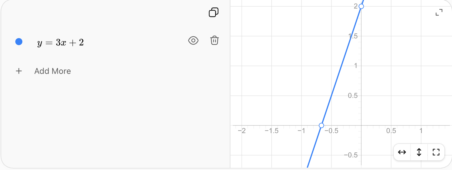
From a Graph to an Equation

To write an equation from a linear graph:

  1. identify the y-intercept
  2. choose two clear points
  3. calculate the slope
  4. substitute into y = mx + b

Suppose a line:

  • crosses the y-axis at 4
  • rises 3 units for every 1 unit to the right

Then:

m = 3

b = 4

Therefore:

y = 3x + 4


From a Graph to a Table

Suppose a graph represents:

y = 2x + 1

Read several points from the graph.

x y
0 1
1 3
2 5
3 7

A table records selected points from the continuous relationship.


From a Graph to Words

Suppose a graph:

  • crosses the y-axis at 10
  • rises by 4 for every increase of 1 in x

A verbal description could be:

"The relationship begins at 10 and increases by 4 units for every 1-unit increase in the input."

If context is provided, the description should include appropriate units.


Comparing Slope Across Representations

Slope may appear differently depending on the representation.

Equation

y = 5x + 2

Slope:

5

Table

x y
0 2
1 7
2 12

Rate:

+5 per +1 in x

Graph

The line rises 5 units for every 1 unit moved right.

Words

"The output increases by 5 for every additional unit of input."

All four describe:

m = 5


Comparing Intercepts Across Representations

The y-intercept also appears differently.

Equation

y = 3x + 8

Intercept:

8

Table

When x = 0:

y = 8

Graph

The line crosses the y-axis at:

(0, 8)

Words

"The initial value is 8."

Again, these are equivalent descriptions of the same feature.


Recognizing Equivalent Representations

Suppose you are given:

Equation A

y = 4x + 3

Table B

x y
0 3
1 7
2 11
3 15

Description C

"The relationship starts at 3 and increases by 4 for every unit increase in x."

All three have:

slope = 4

intercept = 3

Therefore:

A, B, and C are equivalent representations.


Detecting Representations That Are Not Equivalent

Suppose:

Equation

y = 2x + 5

and a table:

x y
0 5
1 8
2 11
3 14

The table has:

slope = 3

intercept = 5

The equation has:

slope = 2

intercept = 5

They share the same starting value but not the same rate of change.

Therefore:

They are not equivalent.


Comparing Linear Relationships

Consider:

Relationship A

y = 2x + 10

Relationship B

y = 5x + 1

Relationship A:

slope = 2

intercept = 10

Relationship B:

slope = 5

intercept = 1

A begins with a larger value.

B changes more quickly.

This means A may initially have the larger output, but B can eventually overtake it.


Finding Where Relationships Are Equal

Using:

A: y = 2x + 10

B: y = 5x + 1

Set the equations equal:

2x + 10 = 5x + 1

Subtract 2x:

10 = 3x + 1

Subtract 1:

9 = 3x

x = 3

Find y:

y = 2(3) + 10

y = 16

The relationships are equal at:

(3, 16)


Seeing the Same Comparison on a Graph

The equations:

y = 2x + 10

and:

y = 5x + 1

can be displayed together.
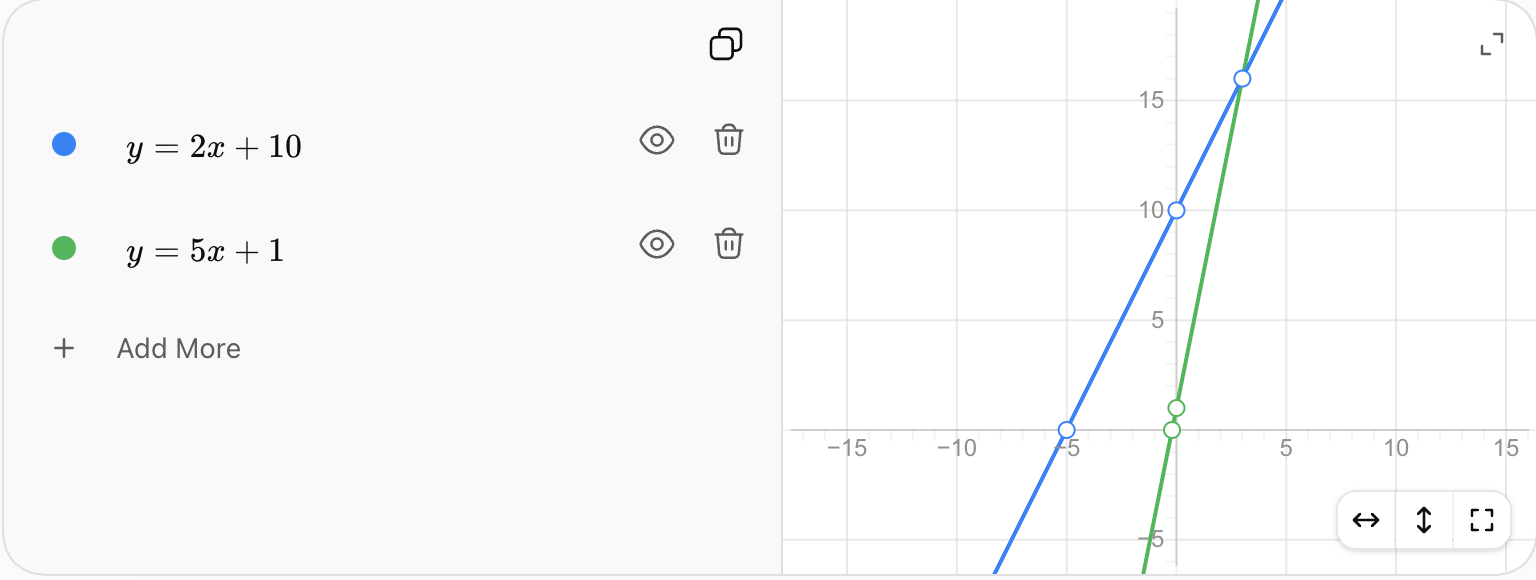
The graph visually shows that:

  • the first relationship starts higher
  • the second has a steeper slope
  • the two relationships eventually meet and then change order

This demonstrates why graphs are useful for comparisons.


Comparing a Table with an Equation

Suppose Plan A is:

A = 4x + 12

Plan B is represented by:

x B
0 5
1 11
2 17
3 23

From the table:

slope = 6

intercept = 5

Therefore:

B = 6x + 5

Now comparison is easier.

Plan A:

m = 4, b = 12

Plan B:

m = 6, b = 5

Plan A starts higher.

Plan B increases faster.


Comparing an Equation with Words

Suppose:

Plan A: C = 8h + 20

Plan B is described as:

"A $10 starting fee plus $12 per hour."

Translate Plan B:

C = 12h + 10

Now compare:

Plan A:

rate = $8/hour

starting fee = $20

Plan B:

rate = $12/hour

starting fee = $10

The equation form makes the mathematical comparison easier.


Comparing Two Tables

Relationship A

x y
0 10
1 13
2 16
3 19

Relationship B

x y
0 2
1 7
2 12
3 17

Relationship A:

m = 3

b = 10

Relationship B:

m = 5

b = 2

Therefore:

  • A has the larger starting value
  • B has the larger rate of change

Using a Common Representation

When comparing relationships shown in different forms, it is often helpful to convert them to a common representation.

For example:

  • convert both to equations
  • convert both to tables
  • graph both relationships together

Equations are especially efficient for comparing slope and intercept.

Graphs are especially effective for comparing overall behaviour and intersections.


Comparing Direct Variation Representations

Recall that direct variation has the form:

y = kx

Suppose a table shows:

x y
1 4
2 8
3 12
4 16

The constant ratio is:

y/x = 4

Therefore:

y = 4x

A verbal description might be:

"The output is four times the input."

A graph would be a straight line through:

(0, 0)

with slope 4.

All representations describe the same proportional relationship.


Distinguishing Proportional and Non-Proportional Linear Relationships

Compare:

A: y = 4x

and:

B: y = 4x + 6

Both are linear.

Both have slope:

4

But only A is proportional.

Why?

A has:

b = 0

and passes through:

(0, 0)

B has:

b = 6

and does not pass through the origin.

Representations can help reveal this distinction.


Real-World Example: Two Taxi Companies

Taxi A charges:

$5 starting fee + $3/km

Therefore:

A = 3d + 5

Taxi B charges:

$9 starting fee + $2/km

Therefore:

B = 2d + 9

Taxi A:

slope = 3

intercept = 5

Taxi B:

slope = 2

intercept = 9

Taxi A starts cheaper but increases more quickly.

Taxi B starts more expensive but increases more slowly.


Finding the Break-Even Distance

Set the taxi costs equal:

3d + 5 = 2d + 9

Subtract 2d:

d + 5 = 9

d = 4

At 4 km:

A = 3(4) + 5 = 17

B = 2(4) + 9 = 17

Therefore, both taxis cost:

$17 at 4 km

For shorter journeys, Taxi A is cheaper.

For longer journeys, Taxi B is cheaper.


Real-World Example: Savings Plans

Plan A begins with:

$200

and adds:

$25/week

Equation:

A = 25w + 200

Plan B begins with:

$80

and adds:

$40/week

Equation:

B = 40w + 80

Plan A has the greater starting value.

Plan B has the greater rate of change.

Different representations can help answer different questions about these plans.


Which Representation Is Best?

There is no single representation that is always best.

The most useful representation depends on what you want to know.

Representation Particularly Useful For
Table exact listed values and patterns
Graph visual trends, comparisons, intersections
Equation calculations, predictions, algebra
Words context, meaning, and units

Strong mathematical reasoning involves choosing the representation that best suits the problem.


When a Table Is Most Useful

Suppose a scientist records temperature every hour.

A table is useful because it preserves the exact measured values.

It allows the scientist to:

  • organize observations
  • compare specific measurements
  • identify possible patterns

However, a table may not make the overall trend as obvious as a graph.


When a Graph Is Most Useful

Suppose you want to compare two savings plans over 20 weeks.

A graph quickly reveals:

  • which starts higher
  • which grows faster
  • when one overtakes the other

This information may be less immediately obvious from a long table.

https://images.openai.com/static-rsc-4/h-o6P3kOUtbeWAAS-4c197aLXvBNyTBYTGjN29-w4xN0VRBHfMG4s3bbuPeWR1txLHnT8iEwP8RIoa7a-4HFrk75RNr3Kw4DcuEu53PnEq41U9KM6evZ7B2C7XdiVE-mVNFlCm6_e5pY32VFvOVcot3vZhQ-Di7W_QeLK8rrd9t2H8ZPH2G9pt-FALsr7phI?purpose=fullsize
 
https://images.openai.com/static-rsc-4/vC6RDfa05bvQFx97coUONWKP7ozkL385yHc4b03IX0iQD3wb55fiI4DOhUZrtVWqaHBTvslijKMb-I21hakcGFDn7IIVxqr9ZBiw6RsBaa0QNz_Ex2dFZBdGzX_3WaaYGKX5n3IqJQ8YLtNaht4G0yvvHPA2JhfGh2J7E7Fjeu5O4IrrlmC2Tl61D0M7CPCi?purpose=fullsize
 
https://images.openai.com/static-rsc-4/GdxHzobAXmQTqu9vFZdc40sOn79Hd4Nr9Xmuu0nO8lIqbtjyUSGA4DoqN9GjYGiW6pNQna1o3MIIThkH_fxkj1FF06Kg6cZRRj7s0MCkB2_rQVHP4VTvHjdRHDdu_T0QNTtYXhumG2nKm5AO7cQsb0AP4KCs9FtaRPdWhd7tkV-r6os0lndJ4EPFNiJmNpz2?purpose=fullsize
 
10

When an Equation Is Most Useful

Suppose you need the exact cost of a 37 km journey.

If:

C = 2.5d + 6

then:

C = 2.5(37) + 6

C = 92.5 + 6

C = $98.50

An equation allows exact calculation without needing a table containing d = 37.


When Words Are Most Useful

Consider:

y = −5x + 100

Without context, we know its mathematical structure but not what it represents.

Now suppose we are told:

"A tank initially contains 100 L and drains at 5 L per minute."

The verbal description gives meaning to:

−5 → water decreases by 5 L/min

100 → initial volume

Words provide the context that the equation alone cannot.


Strengths and Limitations of Tables

Strengths

  • organized
  • easy to read
  • shows exact listed values
  • useful for recognizing patterns
  • useful for recorded data

Limitations

  • shows only selected values
  • may become very long
  • trends may be difficult to see
  • values between rows may not be obvious

Strengths and Limitations of Graphs

Strengths

  • shows overall behaviour
  • makes trends visible
  • makes comparisons easier
  • shows intersections visually
  • shows increasing and decreasing behaviour

Limitations

  • exact values may be difficult to read
  • accuracy depends on scale
  • poor graph scales can be misleading

Strengths and Limitations of Equations

Strengths

  • compact
  • precise
  • allows exact calculations
  • useful for predictions
  • clearly shows mathematical structure

Limitations

  • may not immediately show overall behaviour to a beginner
  • may not explain the real-world meaning
  • requires algebraic understanding

Strengths and Limitations of Verbal Descriptions

Strengths

  • provides context
  • explains units
  • explains meaning
  • connects mathematics to real situations

Limitations

  • can be longer than an equation
  • mathematical structure may be less obvious
  • wording can sometimes be ambiguous

Checking Whether Representations Agree

Suppose an equation is:

y = 6x − 2

and a table claims to represent it:

x y
0 −2
1 4
2 10
3 16

Check:

x = 0:

6(0) − 2 = −2

x = 1:

6(1) − 2 = 4

x = 2:

6(2) − 2 = 10

The values agree.

Therefore, the representations are equivalent.


Finding an Error Between Representations

Suppose:

y = 5x + 3

and a table shows:

x y
0 3
1 8
2 13
3 19

Check x = 3:

5(3) + 3 = 18

But the table says:

19

Therefore, the final row does not match the equation.

Comparing representations is a useful way to detect errors.


Analyzing Rate of Change Across Representations

Suppose three relationships are given.

A

y = 4x + 2

B

"The value begins at 10 and increases by 6 for every unit of x."

C

x y
0 3
2 13
4 23
6 33

Rates:

A:

4

B:

6

C:

m = (13 − 3)/(2 − 0)

m = 10/2

5

Therefore, from greatest to least rate:

B, C, A


Analyzing Starting Values Across Representations

Using the same relationships:

A:

b = 2

B:

starting value = 10

C:

when x = 0:

y = 3

Therefore, from greatest to least starting value:

B, C, A

The representation changes, but the mathematical features can still be compared.


Representations Can Reveal Different Features

Consider:

y = −2x + 12

The equation immediately reveals:

slope = −2

intercept = 12

A table makes specific values easy to read.

A graph makes the decreasing trend obvious.

A verbal description can explain what −2 and 12 mean in context.

The representations are not competing versions of the mathematics. They are different ways of viewing the same relationship.


A Reliable Strategy for Comparing Representations

When comparing tables, graphs, equations, and descriptions:

  1. Identify the variables.
  2. Determine whether the relationship is linear.
  3. Find the rate of change.
  4. Find the starting value or y-intercept.
  5. Record the units if the situation has context.
  6. Convert representations if necessary.
  7. Compare slopes.
  8. Compare intercepts.
  9. Check whether the representations produce the same input-output pairs.
  10. Decide whether they are equivalent.
  11. Choose the representation best suited to the question.
  12. Explain what the mathematical features mean in context.

Common Mistakes

Assuming different-looking representations describe different relationships

A table, equation, graph, and description may all represent exactly the same relationship.

Comparing only one point

Two different lines can share one point. Equivalent linear relationships must have the same slope and intercept.

Comparing only the intercept

Two relationships can start at the same value but change at different rates.

Comparing only the slope

Two parallel relationships can have the same slope but different intercepts.

Using Δy without considering Δx

Rate of change is:

Δy/Δx

Confusing a larger intercept with a larger rate

The intercept describes the starting value. The slope describes how quickly the relationship changes.

Assuming the graph is always the most accurate representation

Graphs are excellent for visualization, but equations and tables may provide more precise numerical values.

Ignoring units

A rate of 5 could mean $5/hour, 5 km/s, or 5 L/min.

Assuming every straight line represents direct variation

A direct variation must also pass through the origin.

Failing to check converted representations

After converting a table or description to an equation, substitute values to verify the result.


Key Terms

Representation — way of showing or communicating a mathematical relationship.

Table — organized display of input-output values.

Graph — visual representation of the relationship between variables.

Equation — mathematical statement describing a relationship between quantities.

Verbal description — explanation of a mathematical relationship using words.

Equivalent representations — different representations describing the same mathematical relationship.

Slope — rate of change of a linear relationship.

Rate of change — change in one variable compared with the change in another.

y-intercept — value of y when x = 0.

Starting value — initial value of the dependent variable.

Linear relationship — relationship with a constant rate of change.

Direct variation — proportional linear relationship of the form y = kx.

Input — independent variable value.

Output — dependent variable value.

Intersection — point where two graphs meet and therefore have the same input and output values.

Conversion — process of changing one representation into another while preserving the same relationship.


Key Takeaways

  • Mathematical relationships can be represented using tables, graphs, equations, and words.
  • Different representations can describe exactly the same relationship.
  • Equivalent linear representations have the same slope and y-intercept.
  • Tables are useful for displaying exact selected values and identifying patterns.
  • Graphs are useful for visualizing trends, rates, and intersections.
  • Equations are useful for exact calculations, predictions, and algebraic analysis.
  • Verbal descriptions provide context, meaning, and units.
  • Linear equations can be written in the form y = mx + b.
  • The slope m appears as a constant rate in tables, steepness on graphs, a coefficient in equations, and a rate in verbal descriptions.
  • The y-intercept b appears as the value when x = 0, the point where a graph crosses the y-axis, the constant term in an equation, and the starting value in words.
  • Converting relationships to a common representation can make comparisons easier.
  • A relationship with a greater starting value does not necessarily have a greater rate of change.
  • A relationship with a greater rate of change may eventually overtake one that starts higher.
  • Intersections represent values for which two relationships have the same output.
  • Comparing representations can help detect errors.
  • A graph may make behaviour easier to see, while an equation may provide greater numerical precision.
  • The best representation depends on the question being investigated.
  • Strong mathematical reasoning involves being able to move flexibly between different representations.

Check Your Understanding

  1. Describe one advantage of representing a relationship using a table, a graph, an equation, and a verbal description.
  2. Write a table containing x = 0, 1, 2, 3, and 4 for:

y = 3x + 5

  1. Write a verbal description of:

y = 4x + 7

that clearly identifies the starting value and rate of change.

  1. Write an equation for the table:
x y
0 6
1 10
2 14
3 18
  1. Determine whether the equation y = 5x + 2 is equivalent to the table:
x y
0 2
1 7
2 12
3 17

Explain how you know.

  1. A relationship is described as: "The value begins at 12 and decreases by 3 for every increase of 1 in x." Write its equation and create a table for x = 0 through x = 4.
  2. Compare y = 2x + 15 and y = 6x + 3. Which has the greater starting value? Which has the greater rate of change?
  3. Relationship A is y = 4x + 8. Relationship B is represented by:
x y
0 2
1 7
2 12
3 17

Write an equation for Relationship B and compare the slopes and intercepts of the two relationships.

  1. A taxi company charges a $7 starting fee plus $3 per kilometre. Represent this relationship using words, an equation, and a table for journeys of 0, 1, 2, 3, and 4 km.
  2. A savings account begins with $150 and increases by $25 each week. Write an equation, construct a table for the first five weeks, and explain how the slope and intercept appear in each representation.
  3. Relationship A is represented by y = 3x + 10. Relationship B begins at 4 and increases by 5 for every unit of x. Determine where the two relationships have the same value.
  4. A student claims that two linear relationships are equivalent because both have a slope of 6. Explain why this information alone is not enough. What else must be compared?
  5. A table shows the points (0, 4), (2, 10), (4, 16), and (6, 22). Determine the equation, describe the relationship in words, and explain what its graph would look like.
  6. Two phone plans are represented differently. Plan A is C = 5g + 20. Plan B has a $35 starting charge and costs an additional $3 per GB. Write both plans as equations, compare their starting costs and rates, and determine the amount of data for which they cost the same.
  7. A tank initially contains 500 L and loses 20 L per minute. Represent the situation with an equation, a verbal description, and a table for the first five minutes. Explain what its graph would show, identify the slope and intercept in each representation, and discuss which representation would be most useful for determining exactly when the tank reaches 100 L.