Measures of Central Tendency and Spread

Сайт: Young Education
Курс: Data and Probability Foundations
Книга: Measures of Central Tendency and Spread
Надруковано: Guest user
Дата: понеділок 9 листопада 2026 16:39 PM

1. Mean (Average)

Learning outcomes
  • I can calculate the mean of a dataset.
  • I can explain what the mean represents.
  • I can interpret averages in real-world situations.
  • I can compare datasets using their means.
  • I can recognize situations where the mean may be misleading.

Mean (Average)

The mean, often called the average, is one of the most common ways to describe a set of numerical data using a single value.

You encounter means in everyday life all the time:

  • average test scores
  • average temperatures
  • average rainfall
  • average travel times
  • average heights
  • average speeds
  • average prices
  • average monthly spending
  • average points scored in a game

The mean helps us answer the question:

"What value could represent the dataset as a whole?"

However, a mean does not tell us everything about a dataset. Two groups can have the same mean while containing very different values, and unusually high or low values can sometimes make the mean misleading.

Understanding the mean therefore involves more than knowing how to calculate it. You also need to know what it represents and when it is useful.

https://images.openai.com/static-rsc-4/gjMyjgKHidseKzhM-XMuJppBo6pRR85N1EGhb85hnwbfZOZbIYEbOKGbHWQP0tAu4hpl63w-qMfrkl83CrLW1DXqwuS4pC9UCDPRxMvYBotuI00LZeDAJSV-dSKW3F7X1p6XHj6OyRRAU9YF6eANlbakAMNNA3jID9wJ9FGkRGFdHRqo159Y5T70Oj_sUboI?purpose=fullsize
 
https://images.openai.com/static-rsc-4/g8AvLYIvg1QXFb9UAKt4m4fNv-oz2ak4c8Rl_dvcn4u35FtFsiNcA3Yi0OOcuGT64Oj51RgXI6MAQSZJafl6cohVsaBmFWeP6Ob7EuUDneYU4OsvV6WFZOtuAPJDrkD4t4ZVb-WN7rEDrwmXvMHnhKl39TJTkOhLRcgiz-Yi7XqHg_j-vITG9TPA_n7fq9eU?purpose=fullsize
 
https://images.openai.com/static-rsc-4/BnZoAPOtM0S8XNQ0ZKYkS14r2x3Zo_TUgxn_L1XO03qs1N_xLNOiDUCzWWsBN_e8JnNQCUr8RjfwEIGMyHP2wqmk4S1r-DRG8XP9YrWn12oJ4czD1oN8VGrbNMprYaEBpzNBpSDd2-aOufuRnuDZgBcpeDGg8I9NVjgkpVrk0zfw11nks0iqVG79fiwdnjNC?purpose=fullsize
 
6

What Is the Mean?

The mean is found by adding all the values in a dataset and then dividing by the number of values.

Mean = sum of all values ÷ number of values

The symbol Σ (Greek capital sigma) is sometimes used to mean "the sum of."

So you may also see:

Mean = Σx ÷ n

where:

  • Σx = sum of all the values
  • n = number of values

For most calculations, however, the important idea is simply:

Add → Count → Divide


Understanding the Mean as Equal Sharing

Another way to understand the mean is as equal sharing.

Suppose four students collect:

2, 4, 6, and 8 samples

Altogether they have:

2 + 4 + 6 + 8 = 20 samples

If the 20 samples were shared equally among the four students:

20 ÷ 4 = 5

So the mean is:

5 samples

The mean can therefore be thought of as the value each member would have if the total were redistributed equally.

This interactive visualization shows that equal-sharing idea directly:
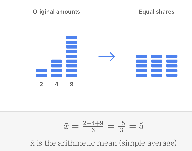
This interpretation is useful because the mean does not have to be one of the original values.

For example:

2, 4, 9

Mean = 15 ÷ 3

Mean = 5

There was no 5 in the original dataset, but 5 represents the value obtained if the total were shared equally.


Calculating the Mean

Consider the dataset:

6, 8, 7, 9, 10

Add the values

6 + 8 + 7 + 9 + 10 = 40

Count the values

There are 5 values.

Divide

Mean = 40 ÷ 5

Mean = 8

A useful routine is:

Add → Count → Divide


Worked Example: Test Scores

Five students receive the following scores:

72, 81, 76, 89, 82

Add the scores:

72 + 81 + 76 + 89 + 82 = 400

Number of scores:

5

Mean = 400 ÷ 5

Mean = 80

We could therefore say:

The mean test score was 80.

Notice that no student actually received exactly 80.

That is completely possible.

The mean is a representative calculated value, not necessarily an observed value.

https://images.openai.com/static-rsc-4/J7VwLefDSVUZ-2RsQk0rErjedub2RNY1djf39TFDvRrKCU01cgik5umEAuDra19AZQRvDhmkOxx-3kR_SqlzO_RYmvauf4zm8BQfZeIi6gzeyZ8hUYO-yYvP3sx_64JtXlYZLtuMm6vKQtZhDbHMusUzV957ViMgzucqZZV4-CpyKg64-cYgs7oh7ge5VzA5?purpose=fullsize
 
https://images.openai.com/static-rsc-4/K4F1g59rbht5LEbOHJ--cBbrSIjxp1Igs6l1G6my39IetlaiHM87c2i6l5rNQpryacU6CASv4UYQh5SfuPsn8aEwArLK8xJn-UalSrW8CCOzeeU1sr_-VbwqNhBxR4MIy829vxIWuClF7VAY8e4DsPN_o9C2DJd7DaSUgQ0ctC6S3KgX92uwgkHcqcU4TM7C?purpose=fullsize
 
https://images.openai.com/static-rsc-4/TYWcDVResgIhTOmaZJWR4T6aJpoRTJstNUWtvdExs_Nzq-fhhcHzWgUJvODU7XM6b3acGrRn0z7ZoBEDUD69Phdq6paSW5saqaYbkI9f9nskpiK4LrVgQotyQkaOyVmhYQIQJ0YQEHBJcg2V3u4HR-9qdCuhIZ3CflZo-0qi4wnUTV7yZ2vOf6L3TT-mkiGH?purpose=fullsize
 
5

The Mean Can Be a Decimal

Consider:

4, 7, 6, 8

Sum:

4 + 7 + 6 + 8 = 25

Number of values:

4

Mean = 25 ÷ 4

Mean = 6.25

The mean does not need to be a whole number.


A Mean Can Be a Value That Is Impossible in Reality

Suppose five families have:

1, 2, 2, 3, 4 children

Total:

1 + 2 + 2 + 3 + 4 = 12

Mean:

12 ÷ 5 = 2.4 children

No family has 2.4 children.

But the mean is still mathematically valid.

It represents the average number of children per family, not the number of children in one particular family.

This is an important idea:

An average describes a dataset. It does not necessarily describe an actual individual member of the dataset.


Why Do We Calculate Means?

Imagine comparing the heights of plants grown under two different conditions.

Group A

14 cm, 15 cm, 13 cm, 16 cm, 17 cm

Group B

19 cm, 20 cm, 18 cm, 21 cm, 22 cm

Looking at every number is possible, but comparing the means makes the overall difference easier to see.

Group A

Mean = (14 + 15 + 13 + 16 + 17) ÷ 5

Mean = 75 ÷ 5

Mean = 15 cm

Group B

Mean = (19 + 20 + 18 + 21 + 22) ÷ 5

Mean = 100 ÷ 5

Mean = 20 cm

We can summarize the data:

Group B had a mean plant height 5 cm greater than Group A.

https://images.openai.com/static-rsc-4/MXYz8IhxnzGzT0ea3pl14MJjc5Fqq0Fs7xNicXw0AVOL6n1gh3aOSSOtfPghIOuOIShs5F35L5p3Mftgm_HLbECEoPyMI_jch9PoHL3BvILPkr8r0fAGOpV0VL_js33V6GUwug51MmGJwIq4nXrjkEn7KMAXWKxjrr0BZOGh4Uio9K-yt7xUmrYwnEF6jlce?purpose=fullsize
 
https://images.openai.com/static-rsc-4/Z6lZg0h51qfuTjWg4fG19d8m-91R8qR2g945XvAkri-BJWQ_e2zDlWVOK5k5CosgDdnDWoq3Ovtbu7GrmLOOPfwKgDi93lCjoNtzU2V8bI_wesWnEAgdgv7YJ-2-KOdLzsjj8ry2yXfy84tq06LwSd-84ZK3vMEWbbUclgSiQXrBU-hFLE3noTIdPSpVJhf3?purpose=fullsize
 
https://images.openai.com/static-rsc-4/f6AX7rNaNaIDfLxROwj2jugkpSjHw2ElP0Qe7zutUgZRKEmUTJDUOobbXlXBO195OPmOZWNRsjI2IE6Mj89SpM5T-Jg7JTQEp2n-ESEwkoMShdS122nWNo6ECcVHSpeeVYPRuqpQaR3cfIG22ENkPE_4fW7D0zTDmE_9GRYPzG5rIyW5ZUwiWZmckcmvQdM_?purpose=fullsize
 
6

Comparing Datasets Using Means

Means are especially useful when comparing groups.

Suppose two basketball teams score the following points over five games.

Team A

70, 75, 80, 85, 90

Mean:

400 ÷ 5 = 80 points

Team B

76, 78, 80, 82, 84

Mean:

400 ÷ 5 = 80 points

Both teams have the same mean:

80 points

Does this mean their performances were identical?

No.

Team A's scores ranged from 70 to 90.

Team B's scores ranged only from 76 to 84.

The averages are identical, but Team B's scores are more tightly grouped.

This demonstrates an important principle:

The mean tells us about the centre of a dataset, but not how spread out the values are.


Mean and Range Together

A useful way to compare datasets is to consider both:

Mean → typical or central value

Range → spread of the data

For the basketball example:

Team A

Mean = 80

Range = 90 − 70 = 20

Team B

Mean = 80

Range = 84 − 76 = 8

Now we have a more complete description.

Both teams have the same mean, but Team B has less variation in its scores.


Using Means in Science

Means are extremely important in scientific investigations.

Suppose a student measures the time required for a toy car to travel a fixed distance.

The student performs five trials:

2.31 s

2.28 s

2.35 s

2.30 s

2.26 s

Sum:

2.31 + 2.28 + 2.35 + 2.30 + 2.26 = 11.50 s

Mean:

11.50 ÷ 5 = 2.30 s

Instead of selecting one trial to represent the experiment, the student can report:

Mean travel time = 2.30 s

Using repeated measurements and calculating a mean can provide a more useful summary than relying on a single trial.

https://images.openai.com/static-rsc-4/EZp_uht1R7QVTUXc1B9BcD7cCX7rDpyItpEmnxf4bePEDuqvq2sDXv6tdquxHohloBHDCeD8Zt8pVY41XgSELTlLoEAWbsqvt_s7hmi51IRnKtcYRG6K4MEDuiJookRuizUI1Ax7Gpsp_0e9Se9gxZoGDtoiDc7FCit0qz-xYdfpgkcl_7f7uO02JjfuHCkj?purpose=fullsize
 
https://images.openai.com/static-rsc-4/HxNK6uTyAa85UEsyCswcwllBArQbsnlfEcko0Y3vLesDE_z7lqDBZZFbzID92Be0-WW65K1ygPMuEE92DC9Yy3dLGvIfIpyFATMW9wrNgYnjfXXF-qSRp_aW9xrrEZFgztdw3tPohEZt3bEDPZsZCWQ7aADu5gsYOR-t90Z93hRazZTEALu-HpLav384U68N?purpose=fullsize
 
https://images.openai.com/static-rsc-4/NjAl-Yv1KdMIDBfC2LPlpR9OKqlmYURsto08lW1FOmnQAUUS3xEkhBBKxogygqfUTVhOmM2L2fLBCdSOpqdN2YHeeMWfMsv8coWSN_LhAce86MSH1kEF-rvJkKtej4q8aITPS-InByFtvPuv1VCX93MV1NMliFBhLYDD3J2SijgQXpWoNDkSZVP_oolKzbFt?purpose=fullsize
 
5

Mean in Real-World Situations

Means help summarize large amounts of information.

Weather

If daily temperatures are:

29 °C, 31 °C, 30 °C, 32 °C, 28 °C

Mean temperature:

(29 + 31 + 30 + 32 + 28) ÷ 5

= 150 ÷ 5

= 30 °C

Travel

Travel times to school:

25 min, 30 min, 28 min, 27 min, 35 min

Mean:

145 ÷ 5

= 29 min

Sports

Points scored:

18, 24, 20, 16, 22

Mean:

100 ÷ 5

= 20 points

Science

Reaction times:

42 s, 39 s, 41 s, 40 s, 43 s

Mean:

205 ÷ 5

= 41 s

In each situation, several measurements are summarized using one representative number.

https://images.openai.com/static-rsc-4/477gDujZFor8M4482GaSfntUuEKfOw7hr6UYMRPvlanUJurSYkqibk0QspReJmUAs4d-G_gHskyRc1TaV3L24nA_J6L5mlt-OMVQF2R0Fa-hfMcxgtMpU_Co4qVE-87_DzfTuK2fQYZ57LpOxjzdu-SBd_erDS_Monm4EIObKu8JaLR960tlCRQdPbjGN9Yx?purpose=fullsize
 
https://images.openai.com/static-rsc-4/-cg8AqPmAJaXRFfn9wwAsEZnQJroEsO_Sx6j4zYMH7_ZFLiqJ1Obnj5ZxyZBJmOlQTQdrl_9n940dP2mFZw1h510-doDQHDex6URD6lcd2ktEi2zfK-Ae1dK_4i2lMGh-ztiFzpjiVgOFdbynlvvt15cyuljuSGiIuQYZ3jQdm2OCZw6y28kKdQfGE4XsJ8D?purpose=fullsize
 
https://images.openai.com/static-rsc-4/EIMpyKXD_QoRnm6hZOoX3yBZNCscaJEZmk-2OgDIqA-2l4nIHPV6dOsOJ-q-nphqdk9U-XB2lFtw3fgmJKcHrFTnZtgIOpOn0_tKngSPeRuYaXJp6EUtUNnR8tPWcfdQAKTcjdaG7RbYulOw3vJ0kTnc9ltavwzl7xyxHkgoXFH0MOkMQx_zhMVhI-ATHuTB?purpose=fullsize
 

Finding a Missing Value Using the Mean

Sometimes you know the mean but one value is missing.

Suppose five test scores have a mean of 80.

The known scores are:

72, 85, 78, 81, ?

If the mean is 80:

Total required = mean × number of values

Total = 80 × 5

Total = 400

Add the known scores:

72 + 85 + 78 + 81 = 316

Missing score:

400 − 316 = 84

Therefore:

Missing score = 84

Check:

(72 + 85 + 78 + 81 + 84) ÷ 5 = 400 ÷ 5

= 80


The Mean Changes When Data Change

Consider:

4, 5, 6

Mean:

15 ÷ 3 = 5

Now increase the final value from 6 to 9:

4, 5, 9

Mean:

18 ÷ 3 = 6

The total increased by 3.

Since there are three values, the mean increased by:

3 ÷ 3 = 1

This shows that every value contributes to the mean.


Adding a Value Equal to the Mean

Consider:

6, 8, 10

Mean:

24 ÷ 3 = 8

Now add another value of 8:

6, 8, 10, 8

Mean:

32 ÷ 4 = 8

The mean does not change.

Why?

Because the new value is exactly equal to the original mean.


Adding a Value Above or Below the Mean

Suppose the mean of a dataset is 20.

If you add a new value:

greater than 20

the mean will increase.

If you add a new value:

less than 20

the mean will decrease.

If you add:

exactly 20

the mean will remain unchanged.

This allows you to predict how new data will affect an average without always calculating the complete mean again.


Outliers and the Mean

An outlier is a value that is unusually high or low compared with the rest of the data.

Consider:

10, 11, 9, 10, 10

Mean:

50 ÷ 5 = 10

Now consider:

10, 11, 9, 10, 50

Mean:

90 ÷ 5 = 18

Most values are still around 9–11.

But the single value 50 has pulled the mean upward dramatically.

This shows that the mean can be sensitive to extreme values.

https://images.openai.com/static-rsc-4/uJisp8TlVbzy0G61iZAEh6ycKVA3myHDd8ZEl-QPaEstL4nnXRrALT-JLXEyFmlTTm04ofiwiNz_vQsdW5gnzbYzx7SIUf0uY3dMeUq6v8u8CQvekEra3HsMnDTOYKHVzss8mGZgLPXF_CW6sABJUJ6zkDrKbXMk2ht1NRZMrhots0SZOa-fy7lezAtbZTs4?purpose=fullsize
 
https://images.openai.com/static-rsc-4/5hF7N2nHNvFvgEIwTEIvPK3A3vfTn2dM20GcZG4HzblCzJaUxGZ8zzMS73egCWvWIvDjZRtvA9eoinGhDqEVko4FNkVHXLcDsxL7v3nn-9rkX8793mZI5ZjE8cq2MJuhzHvlHGdEqUaVbn1-d-CZFv4TH9tF_kg-GPVKvv0fIFWUX6ovu641FIHG3AIZqVqL?purpose=fullsize
 
https://images.openai.com/static-rsc-4/Ek1Y1T_k0mKPcyO0rrv3uxBjnu1c6qD_vxOg25si8ZuRxkjNz5lXGo9sfWDvRpi7mYJGVrpJk6NG8SnVz3uE5cAGhluhCyrYtGi1wqnxQBnbyhsXgPEKFbEY7eahht96qDWgsDWESF-Ltp2hQ9N94NO9Dv_uilNZVkRMrP4UwtAX_5Z4ipDENHCwaGCA-IJj?purpose=fullsize
 
6

When the Mean Can Be Misleading

Consider the annual incomes of five people:

$30,000

$32,000

$35,000

$38,000

$365,000

Total:

$500,000

Mean:

$500,000 ÷ 5 = $100,000

Would it be reasonable to say that a typical person in this group earns about $100,000?

Not really.

Four of the five people earn less than $40,000.

The unusually high income has pulled the mean upward.

The calculation is correct.

The problem is with the interpretation.

This is an important distinction:

A mean can be mathematically correct while still giving a misleading impression of a dataset.


Mean and Median

When extreme values are present, another measure called the median may sometimes describe the centre more effectively.

Consider again:

30,000, 32,000, 35,000, 38,000, 365,000

Mean = 100,000

The median is the middle value:

35,000

In this example, the median is much closer to what most people in the group earn.

This does not mean that the median is always "better."

It means that the most useful measure depends on the shape and purpose of the data.


Mean and Mode

Another measure of central tendency is the mode.

Consider:

4, 5, 5, 5, 7, 8

Mean:

34 ÷ 6 ≈ 5.67

Mode:

5

The mean uses every numerical value.

The mode identifies the most frequently occurring value.

Depending on the question, either may provide useful information.


Measures of Central Tendency

Mean, median, and mode are known as measures of central tendency.

They describe the centre or typical value of data in different ways.

Measure Meaning
Mean Sum of values ÷ number of values
Median Middle value when ordered
Mode Most frequently occurring value

Each answers a slightly different question.

The mean is especially useful when:

  • the data are numerical
  • all values should contribute
  • there are no extreme values severely distorting the result

Comparing Means Carefully

Suppose:

Class A

Mean test score = 76%

Class B

Mean test score = 81%

We can say:

Class B had a higher mean score.

But we should not automatically conclude:

Every student in Class B scored higher than every student in Class A.

The datasets may overlap considerably.

For example, Class A might contain a student scoring 95%, while Class B contains a student scoring 60%.

A mean describes the group, not every individual within it.


Means and Sample Size

Suppose one survey asks five people how many hours they sleep.

Mean = 7.2 hours

Another survey asks 5,000 people.

Mean = 7.2 hours

The means are identical.

But the second result may provide stronger information about the wider population if the sample was selected appropriately.

When interpreting a reported mean, ask:

  • How many observations were included?
  • Who or what was measured?
  • Was the sample representative?
  • Were extreme values present?
  • How much variation was there?

The mean should always be interpreted in the context of the dataset.


Weighted Means

Sometimes values do not contribute equally to an overall average.

Suppose your course grade consists of:

  • homework: 20%
  • project: 30%
  • final test: 50%

If your scores are:

Homework = 90%

Project = 80%

Final test = 70%

You should not simply calculate:

(90 + 80 + 70) ÷ 3 = 80%

because the components have different importance.

Instead:

Homework contribution:

90 × 0.20 = 18

Project contribution:

80 × 0.30 = 24

Final test contribution:

70 × 0.50 = 35

Total:

18 + 24 + 35 = 77

Weighted mean = 77%

A weighted mean gives some values greater influence than others.


Averages Can Hide Important Information

Suppose two science classes complete the same test.

Class A

60, 65, 70, 75, 80

Mean = 70

Class B

40, 40, 70, 100, 100

Mean = 70

The classes have the same mean.

But their score distributions are very different.

Class A's results are relatively clustered.

Class B's results are much more spread out.

Reporting only:

"Both classes averaged 70."

hides this important information.

Whenever possible, examine the original data or measures of spread alongside the mean.


Averages in Headlines and Advertising

You may encounter statements such as:

"The average customer saves $500!"

Before interpreting the claim, ask:

  • Is "average" the mean?
  • How many customers were included?
  • What were the individual savings?
  • Were there extreme values?
  • What time period was used?
  • Were all customers included?
  • How was the sample selected?

The word average can sound convincing while hiding important details about the underlying data.

Good statistical thinking means looking beyond the single number.


Worked Example: Comparing Experimental Results

Two groups measure reaction time.

Group A

12.1 s, 12.3 s, 12.0 s, 12.2 s, 12.4 s

Mean:

(12.1 + 12.3 + 12.0 + 12.2 + 12.4) ÷ 5

= 61.0 ÷ 5

= 12.2 s

Group B

9.0 s, 10.5 s, 12.0 s, 13.5 s, 16.0 s

Mean:

61.0 ÷ 5

= 12.2 s

Again, the means are identical.

But:

Group A range = 12.4 − 12.0 = 0.4 s

Group B range = 16.0 − 9.0 = 7.0 s

Group A's measurements are much more consistent.

This is why scientists should not evaluate experimental data using the mean alone.


Estimating a Mean

Sometimes you may want to estimate a mean quickly.

Consider:

49, 51, 50, 52, 48

Even before calculating, you can see that the values cluster around:

50

So you would expect the mean to be close to 50.

The exact calculation gives:

250 ÷ 5 = 50

Estimating before calculating is useful because it helps you detect mistakes.

If your calculator gave:

500

you would immediately know something had gone wrong.


Checking Whether Your Mean Is Reasonable

For ordinary datasets, the mean should lie between the smallest and largest values.

For example:

12, 15, 18, 20

The mean cannot be:

25

because 25 is greater than every value.

Likewise, it cannot be:

5

because 5 is lower than every value.

A useful check is:

minimum value ≤ mean ≤ maximum value

If your calculated mean lies outside this range, check your calculation.


Common Mistakes

Forgetting to include every value

Every observation must be included unless there is a justified reason for excluding one.

Dividing by the wrong number

Divide by the number of values, not by the largest value or the sum.

Miscounting the data

Repeated numbers still count as separate observations.

For:

4, 4, 6, 7

there are four values, not three different values.

Rounding too early

Keep sufficient decimal places during calculations and round at the end when necessary.

Assuming the mean must appear in the dataset

The mean is calculated and may not be one of the original values.

Assuming "average" always means mean

Average can refer to mean, median, or mode depending on context.

Ignoring outliers

Extreme values can strongly affect the mean.

Comparing groups using only the mean

Datasets with identical means can have very different spreads.

Assuming a higher group mean means every value is higher

Means describe groups, not individual members.

Trusting an average without knowing the dataset

Ask about sample size, spread, outliers, and how the data were collected.


Key Terms

Data — Information collected through measurements, observations, surveys, or other methods.

Dataset — A collection of related data values.

Mean — The sum of all values divided by the number of values.

Average — A general term for a value used to represent a dataset; often used to mean the arithmetic mean.

Arithmetic mean — The standard mean calculated by adding all values and dividing by the number of values.

Sum — The result of adding values together.

Observation — One individual value or measurement in a dataset.

Frequency — The number of times a value occurs.

Central tendency — The tendency of data to cluster around a central or representative value.

Measure of central tendency — A numerical measure used to describe the centre of a dataset, such as mean, median, or mode.

Median — The middle value when data are arranged in numerical order.

Mode — The value occurring most frequently.

Range — The difference between the highest and lowest values.

Spread — The amount of variation among values in a dataset.

Variation — Differences among individual values.

Outlier — A value unusually far from most of the other values.

Extreme value — A particularly high or low value that may strongly influence the mean.

Sample — A group selected from a larger population for investigation.

Sample size — The number of observations included in a sample.

Population — The entire group about which information is being investigated.

Weighted mean — A mean in which some values contribute more strongly than others.

Representative value — A value used to summarize or describe a dataset.

Relative comparison — Comparing values in relation to one another rather than considering only their individual sizes.


Key Takeaways

  • The mean is one way of describing the centre of numerical data.
  • Calculate the mean using Add → Count → Divide.
  • The mean uses every value in the dataset.
  • The mean can be interpreted as the value obtained if the total were shared equally among all observations.
  • A mean does not have to be one of the original data values.
  • A mean can be a decimal even when all original values are whole numbers.
  • Means allow large datasets to be summarized using a single number.
  • Means are useful for comparing groups.
  • A higher mean does not mean that every individual value in one group is higher.
  • Two datasets can have exactly the same mean while having very different distributions.
  • The range provides information about spread that the mean does not.
  • Means are commonly used to summarize repeated measurements in scientific investigations.
  • Every value contributes to the mean.
  • Adding a value above the existing mean raises the mean.
  • Adding a value below the existing mean lowers the mean.
  • Adding a value equal to the existing mean leaves it unchanged.
  • Outliers can strongly affect the mean.
  • A mathematically correct mean can still give a misleading impression of a dataset.
  • The median may sometimes provide a more useful measure of centre when extreme values are present.
  • Mean, median, and mode are different measures of central tendency.
  • Sample size and sampling method should be considered when interpreting averages.
  • Weighted means are used when different values have different levels of importance.
  • A mean should normally lie between the smallest and largest values in the dataset.
  • Good statistical thinking means examining the data behind the average, not simply accepting the reported mean.

The most important questions to ask are:

What is the mean?

What does it represent in this situation?

How spread out are the original values?

Are there any extreme values?

Does the mean give a fair picture of the dataset?


Check Your Understanding

1. Calculate the mean:

8, 12, 10, 14, 6

2. Calculate the mean:

3.5, 4.2, 5.1, 4.8, 2.4

3. Five students score:

68, 74, 82, 91, 85

Calculate the mean score.

4. Explain what the mean represents.

5. Why does the mean not need to be one of the original values?

6. The mean of five values is 12. What is their total?

7. Four scores are:

72, 81, 76, 83

A fifth score is added, producing a mean of 80.

What is the missing score?

8. Dataset A:

10, 11, 12, 13, 14

Dataset B:

2, 7, 12, 17, 22

Calculate the mean of each dataset.

9. Calculate the range of each dataset in Question 8.

10. Explain why the datasets in Questions 8–9 should not be considered identical even though their means are equal.

11. A dataset has a mean of 25. A new value of 40 is added. Will the mean increase, decrease, or stay the same? Explain.

12. A dataset has a mean of 25. A new value of 25 is added. What happens to the mean?

13. Calculate the mean:

8, 9, 9, 10, 44

14. Explain why the mean in Question 13 may give a misleading impression of the typical value.

15. A company states that its employees earn an average salary of $90,000. What additional information would you want before deciding whether $90,000 represents what a typical employee earns?

16. Explain the difference between mean and median.

17. Two classes both have a mean score of 75%. Class A has a range of 8 percentage points while Class B has a range of 42 percentage points. What does this tell you about their results?

18. A student's course contains three components:

Assignments = 80%, weighted 20%

Project = 70%, weighted 30%

Exam = 90%, weighted 50%

Calculate the student's weighted mean.

19. Why is calculating a mean from repeated experimental measurements usually more informative than reporting only one measurement?

20. Challenge: A dataset contains five numbers and has a mean of 18. Four of the numbers are:

12, 16, 19, 21

Determine the fifth number and explain how you found it.

2. Median and Mode

Learning outcomes
  • I can determine the median of a dataset.
  • I can identify the mode of a dataset.
  • I can compare mean, median, and mode.
  • I can select appropriate measures of center for different situations.
  • I can interpret median and mode in context.

Median and Mode

A dataset can often be summarized using a value near its centre. In the previous topic, we used the mean.

But the mean is not the only way to describe the centre of data.

Two other important measures are:

  • median — the middle value
  • mode — the most frequently occurring value

Together, the mean, median, and mode are called measures of central tendency or measures of centre.

Different measures answer different questions. Sometimes the mean gives the most useful description. Sometimes the median or mode tells us much more.

The key is not simply knowing how to calculate them. You need to be able to decide:

Which measure best represents the data in this situation?

https://images.openai.com/static-rsc-4/zaFvChiI3eNM0M2U-3pTuGAIzt1x_zFLJzWRknBfcxGSGdf7CzMv9L8PxD_qp7nRv5Qthn-VCebkMYrI3z09hGeKV8CzG5CHujGsnOBd3FTl1YYNwuwSmqP8mXupGMec9ssOKD20kjtJYp5ZwBfd83Ba9rQKlb9GTvDROrrqqWJjEQOUtXaPQTEsuh5qyiGP?purpose=fullsize
 
https://images.openai.com/static-rsc-4/FPjByKf4O26r7n9CuDsbl90Vq7Vn1SIUTHw5rwNcQ5BWtQYJdpjdm0zsVkSDU8a9g_g-O61lYcKwUq5RDR9XYTiJ0QQbfmOny7m_uwDpCivT5-3Creik02RSv_j8izMWJfwdKKCJvvHqR80NiYD8vtPZGeS-OvDfWQtLKqrmkXGLkn7dcaWOJtqtu5Iex8Yb?purpose=fullsize
 
https://images.openai.com/static-rsc-4/5ltHJ6UPQL3x4m6YeLMxE6tm80d1UNqK7q0kUYOdoaWP9qjpD5kR7cAsOWCiTMfVzcrQxvtaYsXsyMpstnwDruaaxA5-eU6ykft-zuSkmcYePUyMQGvXx3ibrIndjrGOoPoG5XnjyGuBusHigqF5HvvggHqo9pDH46bd5lLeUHygv05WTo8il-GKXdFRgAA7?purpose=fullsize
 
5

What Is the Median?

The median is the middle value when a dataset is arranged in numerical order.

The word median means middle.

Consider:

3, 5, 7, 9, 11

There are five values.

The middle value is:

7

Therefore:

Median = 7

There are two values below 7 and two values above 7.


Always Put the Data in Order First

This is the most important step when finding the median.

Consider:

12, 4, 9, 6, 15

It would be incorrect to simply select 9 because it happens to appear in the middle of the written list.

First arrange the numbers from smallest to largest:

4, 6, 9, 12, 15

Now identify the middle:

Median = 9

In this example the answer happened to remain 9, but that will not always happen.

A useful routine is:

Order → Find the Middle


Worked Example: Odd Number of Values

Find the median:

18, 12, 21, 14, 16, 20, 15

First put the values in order:

12, 14, 15, 16, 18, 20, 21

There are seven values.

The fourth value is in the middle:

Median = 16

Three values lie below 16 and three lie above it.


Finding the Median with an Even Number of Values

What happens if there is no single middle value?

Consider:

4, 6, 8, 10

There are four values.

The two middle values are:

6 and 8

Find the mean of those two numbers:

Median = (6 + 8) ÷ 2

Median = 14 ÷ 2

Median = 7

So when there is an even number of observations:

Order the data → Find the two middle values → Calculate their mean


Worked Example: Even Number of Values

Find the median:

17, 8, 14, 11, 20, 9

Put the values in order:

8, 9, 11, 14, 17, 20

The middle values are:

11 and 14

Median = (11 + 14) ÷ 2

Median = 25 ÷ 2

Median = 12.5

Notice that 12.5 does not appear in the original dataset.

Like the mean, the median does not always have to be an observed value.


Locating the Median Position

For an ordered dataset containing n values, the median position can sometimes be found using:

Median position = (n + 1) ÷ 2

For example, if there are 11 values:

Median position = (11 + 1) ÷ 2

= 12 ÷ 2

= 6

So the sixth value is the median.

For most small datasets, however, simply ordering the values and locating the middle is usually easiest.

https://images.openai.com/static-rsc-4/yqpil5FipkqSvekLXNvHawodSu1YgKK0o1PVBHlByaNf0K3_UkuGHMtYq9ZvrJ18MZMRpa7PRPCM4iUnzxXEnna85hqvrhE_Ej2IokYQhRYpMKE_PHkqQCBlOFDV7rxRb531C38MHyalUhDWO1rlkdwmR2D_zJYHw_P4z_NdB3SeNQjCHlvlblTsmXgzoDc9?purpose=fullsize
 
https://images.openai.com/static-rsc-4/X9lhxlB9awS15vHMJcNn6BGdyFLQY1LciOMDgnraUwZk8qx5waAILfJmEBLJtij_4Fcev4W46t5UrsKKZsXmIuujKF9R57CpYwD9heq833rrczp8_xjNlbHneM_3qTe1XSCela2pioXd2fpv8C5JvcjH8jvJo2YvvFghL3yahXf8UtlXTxtBoHx7TuNO6Ri2?purpose=fullsize
 
https://images.openai.com/static-rsc-4/gUv2Aubty5peC8kUmtlX_UJfSrY2W0b9A1AR4vITTQgpTvRrLJsfYIUYRGQrji1Ku_pVbBdDqdNm9nTp_PosZNsnU3oANxDt40djO3w2neZTCMmTNu6uFswZT36iLN_550_Yj6tHKF19RIjpduHSek2fVJxDjUf1FppvTz_m_3ha5vTVl1XsNaouYhDdPQCp?purpose=fullsize
 
7

What Does the Median Represent?

The median divides an ordered dataset approximately into two halves.

About half of the observations are at or below the median and about half are at or above it.

Suppose the ages of seven participants are:

12, 13, 14, 14, 15, 16, 17

Median = 14

The median tells us that the centre of the ordered ages is 14 years.

It does not mean everyone is 14.

It describes the location of the centre of the dataset.


The Median Is Resistant to Extreme Values

One of the most useful features of the median is that it is less affected by unusually high or low values than the mean.

Consider:

8, 9, 10, 11, 12

Median = 10

Mean = 10

Now replace the final value with 100:

8, 9, 10, 11, 100

Median = 10

Mean = 138 ÷ 5

Mean = 27.6

The extreme value dramatically changes the mean.

But the median remains:

10

This is why the median is often useful for datasets containing outliers or extreme values.


Median Income

Income provides a good real-world example.

Suppose five people earn:

$30,000

$32,000

$35,000

$38,000

$365,000

Mean income:

$500,000 ÷ 5 = $100,000

Median income:

$35,000

Which value better represents what a typical person in this small group earns?

In this case, the median provides useful information because the extremely high income has a large effect on the mean.

This is one reason income and house-price data are often reported using medians.

https://images.openai.com/static-rsc-4/4TLJtzcwNjuaGVSjxZ8iCsJlme6EMWj4suIiAbg79G2HVkdycxPPHNcEXJgmf1y9sbfD2zLytqVhhBlj0zbbpZ78DVnTgUucfM7JRedMc79VzsMdj9mjduGP3jjSGznpN4SsgqsCf28eDZ88GwdNGa5aPN_CTq77kQtW2ZXT4s5keQJO2cEvxbigyA_c_BrN?purpose=fullsize
 
https://images.openai.com/static-rsc-4/WZ7yy1ZP90_eW9PmX-dPcW5KUqBUWV-VC9GFMHlVJGMrO7tUJhae7wZxCIeSpkKf9DB0N5FzWYGrbQ8opVt8PCfeXrygsBAw4DQ3GrXarzGuIrnPzfl6nc5IvJcYJoE7RF9NILumcuQ6B_AIM6bpaB1X4JD88363sEKIqMVkuKlc2DjUpubfOSkpDaDyAx-p?purpose=fullsize
 
https://images.openai.com/static-rsc-4/M9REqGP-Mpf9tXAv_6FbsDybgAR7clTkB-y57IVnG5co1rd4gEJ0P6xjWdqthmHFqtbQ37mL8m3Ugz6k5MpNawO86OFQ2WNCv4Es4Za96SfM_5NSpPOpfV_z9Ce5mudKDVOEPEJT6e5qfamNrYzwlrRVVWze7wOeucOtNBIsSmrjR7-Sk-7nnFdsYVPqRlAi?purpose=fullsize
 
6

What Is the Mode?

The mode is the value that occurs most frequently in a dataset.

Consider:

2, 3, 3, 4, 5

The value 3 occurs twice.

Every other value occurs once.

Therefore:

Mode = 3

A useful way to remember this is:

Mode = Most

The mode is the value that occurs most often.


Worked Example: Finding the Mode

Consider:

12, 14, 11, 14, 15, 14, 13

Count how often each value occurs:

11 → once
12 → once
13 → once
14 → three times
15 → once

Therefore:

Mode = 14

Unlike the median, you do not technically need to put the data in numerical order to find the mode.

However, ordering the data can make repeated values easier to identify.


A Dataset Can Have More Than One Mode

Consider:

2, 2, 3, 4, 4, 5

The values 2 and 4 both occur twice.

No other value occurs as frequently.

Therefore, the dataset has two modes:

2 and 4

A dataset with two modes is called bimodal.


A Dataset Can Have Several Modes

Consider:

1, 1, 2, 2, 3, 3, 4

The values:

1, 2, and 3

all occur twice.

They are all modes.

A dataset with more than two modes may be described as multimodal.

The important rule is:

Every value tied for the highest frequency is a mode.


A Dataset Can Have No Mode

Consider:

3, 5, 7, 9, 11

Every value occurs exactly once.

No value occurs more frequently than the others.

Therefore:

There is no mode.

Do not say:

Mode = 0

Zero would only be the mode if zero actually occurred most frequently in the dataset.


Mode with Categories

The mode has an important advantage over the mean and median.

It can be used with categorical data.

Suppose students are asked for their favourite school subject:

Science, Math, Science, English, Science, Math, Art

Science appears most frequently.

Therefore:

Mode = Science

You cannot calculate a meaningful mean of:

Science + Math + English + Art

But you can identify the mode.

This makes mode especially useful for surveys and categories.

https://images.openai.com/static-rsc-4/16pEVqU9y6sYDVQN2qgw3zYD_57mD2LE1OJCqTymNcb55CoMMl7Dyi1nvZ9wSm5Hr8Rb4NW5HaPiNcQ_ASO2rQwKFd7VkE2T3D7_3qTtuR-kNuyfh2JS68W7QANRt_hu33n8NyatHUUsw5uMHoBiU0dDeIDXqeJpz7bFPBfFGGdp6YOFds4QqGoy-WXgd2Gt?purpose=fullsize
 
https://images.openai.com/static-rsc-4/nfDavtnv7peIrJgaAVO-mnMiGRAIsdwADUyeHN636_LhhmMivZA0Rdn3GMd7VEwuNklHwpgCcJEqPvWXxevZYWSTXW41BKfb4BHOChtGyzBkeoTrP6rh_OtnWpgL8JEQVYhUQTDhD_Gb5-R0TG7jJ-RyAAs-RrDTvU__2w_Z75liLF7e7_n-QBewwGvnzcdj?purpose=fullsize
 
https://images.openai.com/static-rsc-4/9pmF4tX-47dkHHSyNyXIJjYo_YqHLcAielzjSQioSdmTWiXujYzAiK8PB9GIK8cmfIytartOrmXXVxLrdE8XbnoqmpHXV_n-vDBWiRJ0EPA9R0cnf_7m1DUsVAdjgVxZWs-UoASEVvQwUs2vllRTH-mVYrSBO3rWJCbYZY0bXyA3IsynuFyWTq379VGkqF76?purpose=fullsize
 
5

Mode in Everyday Life

Businesses may use the mode to identify:

  • most popular shoe size
  • most frequently purchased product
  • most common clothing size
  • most popular colour
  • most common order
  • most frequently selected menu item

Suppose a shoe shop records these sizes sold:

7, 8, 8, 9, 8, 10, 9, 8, 11

Mode = 8

Knowing the mode may help the store decide which shoe size it needs to stock in larger quantities.


Comparing Mean, Median, and Mode

Consider:

2, 3, 3, 4, 8

Mean

Mean = (2 + 3 + 3 + 4 + 8) ÷ 5

Mean = 20 ÷ 5

Mean = 4

Median

Ordered data:

2, 3, 3, 4, 8

Middle value:

Median = 3

Mode

Most frequent value:

Mode = 3

So:

Mean = 4

Median = 3

Mode = 3

All three describe the dataset in different ways.


What Each Measure Tells Us

Mean

The mean uses every numerical value.

It answers:

What would each value be if the total were shared equally?

Median

The median uses the position of values.

It answers:

What is the middle of the ordered dataset?

Mode

The mode uses frequency.

It answers:

Which value or category occurs most often?

These are related ideas, but they are not interchangeable.


Mean, Median, and Mode Can Be Equal

Consider:

2, 3, 4, 4, 4, 5, 6

Mean:

28 ÷ 7 = 4

Median:

4

Mode:

4

Therefore:

Mean = Median = Mode = 4

This often happens in datasets that are reasonably balanced around a central value.


Mean, Median, and Mode Can Be Different

Consider:

2, 3, 3, 4, 18

Mean:

30 ÷ 5 = 6

Median:

3

Mode:

3

The extreme value 18 has pulled the mean upward.

This difference between the measures gives us useful information about the shape of the dataset.

https://images.openai.com/static-rsc-4/fFPM38Drn5RpAKDs484l_kJjDVAL_vtA5VcS1Lq60up6fstuplA_dp59cEk0XoBWKATMqPGIxNQHywc5hksoNN4UFIVX_0iIIOXOb10iIIC3k4avHNH4vAMFfHiCAuvVieV1xXfloVExBwv4GnEqBLIc63zJDQ1-th_vGmNKVUziZ8IAJW2JYsrgsse-ziYD?purpose=fullsize
 
https://images.openai.com/static-rsc-4/6J8KqS3Fbcp1i-C_qB-4R4dxlOrweictQm9NUSEf7XufJtY9ieIP-EgXYuZRQkBZSYVrJpDiw9qT5DoLG-xWhfpSrZm-MJHmcIPp94eRc-hr6ovgLdQKInyPQ_Jm-3sFutUDkb_amlncJmzhNqRoo7JnsVE2p3hwiPwF6vMkmTXsS2rox0sRfLTPRcoHSrex?purpose=fullsize
 
https://images.openai.com/static-rsc-4/nyD30OJqsAodujF6Bett4bgKNNcO0Dw8b3Afd6C1ehGFKso03AtdxydSRhJxJaDFC4f9rP6ExkLbKSc725L_SR8Hmj_zC7lm5UA9bLO3qd0Xq_WBiP4yfok4ilHu907lj2kXV0cJQYW0BEad_vw1WqfGzCiWFA8rQAPYoK-p7due2rNpAVzF2wUlqT2_8eTE?purpose=fullsize
 
5

Choosing the Best Measure of Centre

There is no rule saying that one measure is always best.

The appropriate measure depends on:

  • the type of data
  • the distribution of the values
  • whether extreme values are present
  • what question you are trying to answer

When the Mean Is Useful

The mean is often useful when:

  • the data are numerical
  • most values are reasonably clustered
  • there are no extreme outliers
  • every measurement should contribute to the result

Example:

Repeated measurements:

10.1 s, 10.3 s, 10.2 s, 10.4 s, 10.0 s

The mean provides a useful summary because the values are relatively close together.


When the Median Is Useful

The median is often useful when:

  • extreme values are present
  • the distribution is skewed
  • you want the middle position
  • a few unusually high or low values would distort the mean

Examples include:

  • household income
  • house prices
  • travel times
  • waiting times

Suppose houses sell for:

$300,000, $320,000, $340,000, $350,000, $2,000,000

The mean is heavily influenced by the $2 million property.

The median:

$340,000

may better describe the centre of these particular sale prices.


When the Mode Is Useful

The mode is useful when you want to know:

What occurs most frequently?

It is especially useful for:

  • categories
  • product sizes
  • survey responses
  • common choices
  • frequently occurring values

For example:

T-shirt sizes sold:

M, L, M, S, M, L, XL, M

Mode = M

The mean and median would not be meaningful for these category labels.


Choosing the Measure Based on the Question

Consider a shoe store.

The manager wants to know:

Which shoe size should we stock most heavily?

The mode is probably useful because it identifies the most commonly purchased size.

Now consider:

What is the middle house price in this neighbourhood?

The median directly answers that question and is less affected by unusually expensive houses.

Now consider:

What was the average reaction time across repeated laboratory trials?

The mean may be appropriate because all numerical measurements contribute.

The correct measure depends on what you want to know.


Worked Example: House Prices

Suppose six houses sell for:

$280,000

$300,000

$310,000

$330,000

$340,000

$1,200,000

Mean

Total = $2,760,000

Mean = $2,760,000 ÷ 6

Mean = $460,000

Median

The middle values are:

$310,000 and $330,000

Median = ($310,000 + $330,000) ÷ 2

Median = $320,000

The mean suggests $460,000.

But five of the six houses sold for $340,000 or less.

In this situation, the median gives important information about the centre because the expensive house strongly influences the mean.


Worked Example: Test Scores

Consider:

68, 71, 74, 76, 76, 78, 81

Mean:

524 ÷ 7 ≈ 74.9

Median:

76

Mode:

76

All three values are relatively close.

There are no extreme values dramatically changing the mean.

In this case, all three measures provide useful information, although each describes the dataset differently.


Worked Example: Product Sales

A shop sells T-shirts in the following sizes:

S, M, M, L, M, XL, L, M, S, M

Which measure should the manager use to determine the most popular size?

Mean?

No. You cannot meaningfully average clothing categories.

Median?

Not usually the most useful choice for this question.

Mode?

Yes.

Mode = M

Therefore, medium is the most frequently sold size.


The Median Does Not Consider the Size of Every Value

The median depends mainly on position, not on how extreme the largest and smallest values are.

Compare:

Dataset A

1, 5, 6, 7, 10

Median = 6

Dataset B

−500, 5, 6, 7, 10,000

Median = 6

The extreme values changed dramatically.

The median did not change at all.

This resistance to extreme values is both a strength and a limitation.

It makes the median useful when outliers exist, but it also means the median does not reflect the magnitude of every observation.


The Mode Does Not Have to Be Near the Centre

Consider:

1, 1, 1, 10, 11, 12, 13

Mode = 1

Median = 10

The mode is not necessarily near the mathematical centre of the dataset.

It simply tells us which value occurs most frequently.

This is why you should interpret the word centre carefully when discussing measures of central tendency.


Frequency Tables

The mode can be particularly easy to identify from a frequency table.

Number of Books Read Frequency
0 2
1 5
2 8
3 6
4 3

The highest frequency is:

8

This corresponds to:

2 books

Therefore:

Mode = 2 books

The frequency itself is not the mode.

The mode is the value associated with the highest frequency.


Finding the Median from a Frequency Table

Consider:

Score Frequency
1 2
2 3
3 4
4 2

There are:

2 + 3 + 4 + 2 = 11 observations

The median is the sixth observation.

Expanded data:

1, 1, 2, 2, 2, 3, 3, 3, 3, 4, 4

The sixth value is:

3

Therefore:

Median = 3

You do not always need to write out the entire dataset, but doing so can help while learning.


Interpreting the Median in Context

Suppose the median waiting time at a clinic is:

18 minutes

A useful interpretation is:

The middle waiting time was 18 minutes when the waiting times were ordered.

It does not mean:

  • everyone waited 18 minutes
  • the mean was necessarily 18 minutes
  • 18 minutes was necessarily the most common waiting time

Always interpret the statistic according to what it actually measures.


Interpreting the Mode in Context

Suppose the mode of shoe sizes sold is:

Size 9

A useful interpretation is:

Size 9 was the most frequently sold shoe size in the dataset.

It does not mean:

  • the average customer wears size 9
  • half of customers wear size 9
  • size 9 is the middle size

Mode tells us about frequency, not position or equal sharing.


Comparing Two Datasets

Consider:

Dataset A

4, 5, 5, 6, 10

Mean = 6

Median = 5

Mode = 5

Dataset B

5, 5, 6, 7, 7

Mean = 6

Median = 6

Modes = 5 and 7

Both datasets have the same mean.

But their medians and modes differ.

This demonstrates why looking at multiple measures can reveal information hidden by a single average.


Outliers and Measures of Centre

Suppose a class records:

12, 13, 14, 14, 15, 16, 60

Mean:

144 ÷ 7 ≈ 20.6

Median:

14

Mode:

14

The value 60 strongly affects the mean.

It does not affect the median nearly as much and does not change the mode.

When outliers are present, compare several measures before deciding how to summarize the data.

https://images.openai.com/static-rsc-4/5hF7N2nHNvFvgEIwTEIvPK3A3vfTn2dM20GcZG4HzblCzJaUxGZ8zzMS73egCWvWIvDjZRtvA9eoinGhDqEVko4FNkVHXLcDsxL7v3nn-9rkX8793mZI5ZjE8cq2MJuhzHvlHGdEqUaVbn1-d-CZFv4TH9tF_kg-GPVKvv0fIFWUX6ovu641FIHG3AIZqVqL?purpose=fullsize
 
https://images.openai.com/static-rsc-4/JLS-BoT1gTzxX-Q22Yc6a8RvEcH5qZz0QFpWPrDBGDSChga0rBKXY-VGRUraJnguhtbbPr0SMQIcnGAQMsUs6ra-64AbJHf7716X2nz3uWSzME9IOR_6dhQzRuvpuTusMNLBSc_0MIU1V7rkNs1mVOwPOFfwkdb9MjGSf3XkVk2ca5BLCFETvRjzzqZa1Pue?purpose=fullsize
 
https://images.openai.com/static-rsc-4/ZvMtTE_E72wThQxX1_xv84btani7pYrdCHT8VsaluU79chyyBY9ocwzgSXedDCccX8GFMT7AEY-9p80kjhAfRM2muSdnD06Kn3cnOurPEdZkke-sgaKlyX2tIs0H-qmOXEK3pQk3vMggCq3IXxnNezYl66e1PUbaf8GskKTCL0URP51v73v3hTDyv-kUEArp?purpose=fullsize
 
5

Real-World Example: Travel Times

Suppose travel times to school are:

18, 19, 20, 20, 21, 22, 65 minutes

Mean:

185 ÷ 7 ≈ 26.4 minutes

Median:

20 minutes

Mode:

20 minutes

Why was one trip 65 minutes?

Perhaps there was:

  • a traffic accident
  • severe weather
  • a bus delay

If you want to describe a typical journey, the median of 20 minutes may be more informative than the mean of 26.4 minutes.

But the 65-minute trip is still real data and may be important depending on the question.


No Measure Is Automatically "Correct"

Suppose someone asks:

"What is the average?"

A useful response may be:

"Which average do you mean?"

Mean, median, and mode all describe data differently.

For example, a business may care about:

Mean sale value — useful for revenue calculations.

Median sale value — useful for describing a typical transaction when extreme sales occur.

Mode product — useful for identifying the most commonly purchased item.

All three can be useful simultaneously.


Common Mistakes

Forgetting to order data before finding the median

Always arrange numerical data before locating the middle.

Choosing one of the middle values when there is an even number

Calculate the mean of the two middle values.

Assuming the median must appear in the dataset

With an even number of observations, it may fall between two values.

Saying the mode is the largest number

Mode means most frequent, not largest.

Saying the mode is the highest frequency

The mode is the value associated with the highest frequency.

Saying the mode is zero when there is no mode

"No mode" and "mode = 0" mean very different things.

Assuming there can only be one mode

Datasets can be bimodal or multimodal.

Assuming every dataset has a mode

Some datasets have no mode.

Assuming the median is always better than the mean

The appropriate measure depends on the data and the question.

Ignoring extreme values

Outliers can strongly affect the mean.

Using the mean with categories

You cannot meaningfully calculate the mean of categories such as colours or favourite subjects.

Assuming equal means imply equal datasets

Datasets can have the same mean while having different medians, modes, ranges, and distributions.


Key Terms

Measure of centre — A value used to describe the central or typical part of a dataset.

Central tendency — The tendency of data to cluster around a central value.

Mean — The sum of all numerical values divided by the number of values.

Median — The middle value of an ordered dataset.

Mode — The value or category occurring most frequently.

Average — A general term for a value used to represent a dataset; it may refer to mean, median, or mode depending on context.

Ordered data — Data arranged from smallest to largest or largest to smallest.

Frequency — The number of times a value or category occurs.

Frequency table — A table showing values or categories and how often they occur.

Unimodal — Having one mode.

Bimodal — Having two modes.

Multimodal — Having more than two modes.

No mode — A situation in which no value occurs more frequently than the others.

Outlier — A value unusually far from most other observations.

Extreme value — A particularly high or low observation.

Range — The difference between the largest and smallest values.

Distribution — The way values are spread throughout a dataset.

Skewed data — Data whose distribution extends farther in one direction than the other.

Categorical data — Data representing groups or categories rather than numerical measurements.

Numerical data — Data represented using numbers with quantitative meaning.

Representative value — A value used to summarize or describe a dataset.

Robust/Resistant measure — A statistic that is relatively unaffected by extreme values; the median is more resistant to outliers than the mean.


Key Takeaways

  • Mean, median, and mode are measures used to summarize data.
  • The median is the middle value of an ordered dataset.
  • Always put numerical data in order before finding the median.
  • With an odd number of values, the median is the single middle value.
  • With an even number of values, calculate the mean of the two middle values.
  • The median does not necessarily appear in the original dataset.
  • The median is less affected by extreme values than the mean.
  • This makes the median useful for datasets containing strong outliers or skewed values.
  • The mode is the value or category occurring most frequently.
  • A dataset can have one mode, several modes, or no mode.
  • The mode can be used with categorical data.
  • Mean, median, and mode describe different features of a dataset.
  • The mean uses the numerical size of every value.
  • The median depends mainly on the position of values.
  • The mode depends on frequency.
  • The mean is often useful when numerical data contain no extreme values.
  • The median is often useful when extreme values strongly influence the mean.
  • The mode is particularly useful when you want to identify the most common value or category.
  • A higher or lower mean does not tell you everything about a dataset.
  • Two datasets can have identical means but different medians, modes, and distributions.
  • No single measure of centre is automatically best.
  • The appropriate measure depends on both the data and the question being asked.
  • Statistics should always be interpreted in their real-world context.

A useful way to remember the three measures is:

Mean → Equal sharing

Median → Middle

Mode → Most common

The important question is not simply:

"Can I calculate all three?"

It is:

"Which measure gives the most useful description of these data, and why?"


Check Your Understanding

1. Find the median:

3, 7, 5, 9, 4

2. Find the median:

12, 8, 15, 11, 20, 9

3. Find the mode:

4, 7, 4, 8, 6, 4, 9

4. Find the mode:

2, 3, 3, 5, 5, 7

5. Does this dataset have a mode?

1, 3, 5, 7, 9

Explain your answer.

6. Calculate the mean, median, and mode:

3, 4, 4, 5, 9

7. Calculate the mean and median:

8, 9, 10, 11, 100

Which measure better represents the centre of most of these values? Explain.

8. Why must numerical data be ordered before finding the median?

9. Explain why the median is less affected by extreme values than the mean.

10. A neighbourhood has these house prices:

$280,000, $300,000, $315,000, $325,000, $340,000, $2,000,000

Calculate the median.

11. Would the mean or median provide more useful information about the centre of these house prices? Explain using the data.

12. A shoe shop sells these sizes:

7, 8, 9, 8, 10, 8, 9, 11, 8

Find the mode and explain what it means to the shop manager.

13. Why can the mode be used with favourite colours but the mean cannot?

14. A dataset has two values tied for the highest frequency. What is this called?

15. Explain the difference between what the mean, median, and mode represent.

16. The median waiting time at a restaurant is 24 minutes. Explain what this tells you about the dataset.

17. Dataset A has a mean of 15 and Dataset B also has a mean of 15. Give one reason why the two datasets could still be very different.

18. Which measure would probably be most useful for each situation? Explain your choices.

a. Most popular T-shirt size
b. Typical house price when several extremely expensive homes are included
c. Average time from several consistent laboratory trials

19. A dataset has the following frequency table:

Score Frequency
1 3
2 5
3 8
4 4
5 2

Identify the mode.

20. Challenge: Consider:

4, 5, 5, 6, 7, 8, 50

Calculate the mean, median, and mode. Then explain which measure you would choose to represent a typical value in this dataset and justify your choice using the distribution of the data.


3. Range and Variability

Learning outcomes
  • I can calculate the range of a dataset.
  • I can explain the concept of variability.
  • I can compare datasets using measures of spread.
  • I can interpret differences in variability.
  • I can explain why variability is important when analyzing data.

Range and Variability

When we analyze data, knowing the centre of a dataset is useful—but it does not tell us the whole story.

Consider these two datasets:

Dataset A: 8, 9, 10, 11, 12

Dataset B: 2, 6, 10, 14, 18

Both have exactly the same mean:

Mean = 10

But the datasets are clearly different.

Dataset A is tightly clustered around 10.

Dataset B is much more spread out.

This difference is called variability.

Variability describes how much the values in a dataset differ from one another. Measures of spread, such as the range, help us describe this variability numerically.

Understanding variability is essential because two datasets with the same mean or median can represent very different situations.

https://images.openai.com/static-rsc-4/xwtSFGLCz2tJV3dsHntU7s79gJKEiRmoZZSBxu9D5BBl3LkLELrFlGPs0OMpyZf85dssTA4AsBNu0MrUzmwu7jkqnOYZw1-APrKgvf5wpnyiU6XbuxyFvK-O7Kk5fbxI7dD1qJ_7meaJ0NsnKdFdWTX5eoeAZC3TqbuHVCOEoAAb7PWXC0BJKhmNHCWFaFC9?purpose=fullsize
 
https://images.openai.com/static-rsc-4/YuoFu4wBEx3UAydWpCYemEu3T6ExVXJ_B5AEj0A9B7m3tTBsdnTgbTltiLLx8kPKofJ298sME55OoX69sUPksEWuzAPyOxWjQscyH5UadU3fql7RDRWogFnoFwFxpORIH5aoMWJug6_Xl42dClupoeClX-nfV5wcsMyRiAmZy-HOALEDIo44LrfKbTfI8BO7?purpose=fullsize
 
https://images.openai.com/static-rsc-4/96XqU2pjGhgrzrjFn4mOFa69f1XLqhk5VWLISUI7r5raiU4oxdgKkAn8zwcO8T84WYp4in2CPc14vTu4zIQOKpDxNZbVFcvj5U-h3gk0LNjIp8DyLyImvESWlE8LRdNnzy0JURgMm8TMhrMqQTVU4yZM3AkWDc3GAWXYQsnTiBrT93vn1LyOATt3w796VveW?purpose=fullsize
 
4

What Is Variability?

Variability describes the amount of difference or spread among values in a dataset.

Consider:

10, 10, 10, 10, 10

There is no variability.

Every value is identical.

Now consider:

8, 9, 10, 11, 12

There is some variability.

Now:

−10, 0, 10, 20, 30

There is much greater variability.

As the observations become more spread out, variability generally increases.


Why Variability Matters

Suppose two students each have an average quiz score of 80%.

Student A

78%, 80%, 81%, 79%, 82%

Student B

50%, 65%, 80%, 95%, 110%

Ignoring the unusual grading scale in the example, both could have the same mean, but their performances are very different.

Student A is relatively consistent.

Student B's results vary considerably.

If we looked only at the mean, we would miss this important information.

This is why data analysis often considers:

centre + spread

rather than centre alone.


What Is the Range?

The range is one of the simplest measures of spread.

Range = highest value − lowest value

For example:

4, 7, 9, 10, 13

Highest value = 13

Lowest value = 4

Range = 13 − 4

Range = 9

This tells us that there are 9 units between the smallest and largest values.


Calculating the Range

A useful routine is:

Find the highest → Find the lowest → Subtract

Consider:

18, 12, 25, 16, 20

It may help to order the data:

12, 16, 18, 20, 25

Highest = 25

Lowest = 12

Range = 25 − 12

Range = 13

Unlike finding the median, ordering the data is not strictly necessary.

But it makes identifying the minimum and maximum much easier.


Worked Example: Test Scores

Five students receive:

72, 81, 68, 90, 76

Lowest score = 68

Highest score = 90

Range = 90 − 68

Range = 22 percentage points

This tells us how far apart the highest and lowest scores are.

https://images.openai.com/static-rsc-4/_3rDy5Erwr5K1n_ParNPHCLgOBBTHhfRclNVccK8KvJIp4h46BD_7Gg47afNs4BKlwwWowfqhdSBTYb2dSSyzxeLMG6lIOkCuWofvan-qRcXF5c8_fNIR93f7pKVkYOizTyM7Yrz_urGoWD7Xd4CpMYR3l5jxEI0-QuxwAztsl4werSKvjJOeEMDoXqelo_v?purpose=fullsize
 
https://images.openai.com/static-rsc-4/jGDSSlnmyf8XQo1cmthh7x7U1c2FBCHVGgRFylOWLNCNKpMfLAPvpl5AUtLcr4AiNF483d6mX4eGxusINhzubWntbyakqZmfNHqvU0jFnhr4p2GA_zKCDXRAK8CM_Zl1p6rIvg5W5Qj1JogbtUoZKswvJWXblisPpWo6-5mFOmd7Sl5AfYWEVCIA6aIMI75u?purpose=fullsize
 
https://images.openai.com/static-rsc-4/RybdOh8vjjv_Jy1U8ZTOY5OIcYZsAxM-1dEk8z9BdzweNmzYbBEi1wcpYE4W4agIbkfES0MoYNg5I9Mitbm-ra5ADEEuaGMe7_U2hSXVuFk5Iy1xIDIk105XtV2DFwHjSemRC8qNB-XMUNxXFj0t-IM-Y0y3lF-wbpCu1rm8qWnVlAqCpsK2Y68AesFG9Qee?purpose=fullsize
 
5

Worked Example: Temperature

Suppose temperatures recorded during one day are:

24 °C, 27 °C, 30 °C, 32 °C, 29 °C, 25 °C

Lowest = 24 °C

Highest = 32 °C

Range = 32 − 24

Range = 8 °C

The temperatures varied across an interval of 8 °C.


Range with Negative Numbers

Be careful when the lowest value is negative.

Consider:

−8, −3, 2, 5, 9

Highest = 9

Lowest = −8

Range = 9 − (−8)

Range = 9 + 8

Range = 17

A common mistake is calculating:

9 − 8 = 1

Remember that the lowest value is negative eight, not positive eight.


Range Can Be Zero

Consider:

7, 7, 7, 7, 7

Highest = 7

Lowest = 7

Range = 7 − 7

Range = 0

A range of zero means there is no spread between the highest and lowest values.

Every observation is the same.


Comparing Datasets Using Range

Consider:

Dataset A

18, 19, 20, 21, 22

Mean = 20

Range = 22 − 18

Range = 4

Dataset B

5, 10, 20, 30, 35

Mean = 20

Range = 35 − 5

Range = 30

Both datasets have the same mean.

But Dataset B has a much larger range.

We can say:

Dataset B shows greater variability based on the range.

https://images.openai.com/static-rsc-4/vPQ1USHMx_Nm1rMkyOBj4c2WQAisKZAq3U7UAgQIxOrfZnoSMQKr843q1spbNWLggQN9ofP8Yqj3wt7WjWtUDVOGvRRvuerI3jtfTj5mkxmRQZwTPWbliam4l9qkAaBjsJ4hmV4ZrCxnjTGFH8PaM9aNk5g823pOys3squPSh0KkM5EfJ3f731BYo_9EgUbG?purpose=fullsize
 
https://images.openai.com/static-rsc-4/xwtSFGLCz2tJV3dsHntU7s79gJKEiRmoZZSBxu9D5BBl3LkLELrFlGPs0OMpyZf85dssTA4AsBNu0MrUzmwu7jkqnOYZw1-APrKgvf5wpnyiU6XbuxyFvK-O7Kk5fbxI7dD1qJ_7meaJ0NsnKdFdWTX5eoeAZC3TqbuHVCOEoAAb7PWXC0BJKhmNHCWFaFC9?purpose=fullsize
 
https://images.openai.com/static-rsc-4/QfXv7UOzEnzutptU_C0S2aX1WumYCTdPKNV6u90poVHFZlO7cf8wWWAW4V8nfxQ854QT2Tc7ju2bvBN2x3JJGhgjULgSLVw6ugMU2GbzP-SYVV5L7e9j8uTknxlWZR3pX9Wzmbt8lRE_CMxuUx-oo6VXAgZ0ajR2R0xqaR4hUWl3VSYNUgqNsS8-c4NA1DFc?purpose=fullsize
 
5

Centre and Spread Work Together

Measures of centre include:

  • mean
  • median
  • mode

Measures of spread describe how much values vary.

At this level, the main measure of spread we are using is:

range

Suppose:

Class A

Mean = 75%

Range = 8 percentage points

Class B

Mean = 75%

Range = 42 percentage points

The classes have the same mean.

But Class A's results are much more tightly grouped.

Class B's results show much greater variability.

Reporting both statistics gives a much clearer picture:

Class A: mean = 75%, range = 8

Class B: mean = 75%, range = 42


Low Variability

A dataset with low variability has values relatively close together.

For example:

48, 49, 50, 50, 51, 52

The results are clustered around approximately 50.

Low variability can indicate:

  • consistent measurements
  • similar individuals
  • stable conditions
  • predictable results

However, low variability is not automatically "good."

Whether it is desirable depends on the situation.


High Variability

A dataset with high variability contains values that are more widely spread.

For example:

20, 31, 48, 63, 79

High variability might result from:

  • natural differences
  • inconsistent measurements
  • changing conditions
  • uncontrolled variables
  • different groups within the sample
  • measurement error

High variability is not automatically "bad."

It is information that needs to be explained and interpreted.


Variability in Scientific Experiments

Suppose a student measures the time required for a pendulum to complete ten oscillations.

Experiment A

12.1 s
12.2 s
12.0 s
12.1 s
12.2 s

Range:

12.2 − 12.0 = 0.2 s

Experiment B

10.8 s
11.7 s
12.1 s
12.9 s
13.5 s

Range:

13.5 − 10.8 = 2.7 s

Experiment B shows much greater variability.

That should make the scientist ask:

Why?

Possible explanations include:

  • inconsistent release position
  • timing errors
  • changing pendulum length
  • counting mistakes
  • changing experimental conditions
https://images.openai.com/static-rsc-4/JKCXgLm93tlgXc02xCsr4r7-Xgz205pGWzzCy1y2dsghu9m-l3-Nymoa48FJ_6300ntt_NpOuSIEeLIseDOCG4Oo9xP6qVafVEIiESPy2qT3EV-U5cUdOKZbCXNpKGxkYyr9HGaRtGPsHxaUYM_sMMWMfmjctqqlOJkz7DBI71EJ2tZcpK54mIronWtFpFSU?purpose=fullsize
 
https://images.openai.com/static-rsc-4/e85mUryyMnupXytHEtVxaj2lFu1_idwXvNxzDppCTm_aOd-01438uC1zet9wQ3wXobrtxJpnGFNl_RiYmny9rWF1xuXVgy0LrLil2XZumDy8MyfKziXCWBpk6bK5bqeQZmpMg83wZ1EhqJSERAXKKdf8rATpGTSgTlWTyGFFl5X7GxeeozeOeDvyVxbtrX7L?purpose=fullsize
 
https://images.openai.com/static-rsc-4/k3N861-47smY1jkvK6PToSELsOAg9j5R47nE8eX4AKd98C7rlOxdAM0ENIJZ4WAq5uP15bDok5268rPsaLdU0TXlRFz2Rt38luvCbufPApU62fd-JeT1jb0suKlthk1bpK1JtHBBmj_lDSt37Tw79bgXt0BqvrZNfK9RG7Y-sqlzh2XW_POca6v0PZzVONAO?purpose=fullsize
 
5

Variability Is Not Always Experimental Error

Suppose you measure the heights of 100 students.

The heights will vary.

That does not mean the measurements are necessarily poor.

Humans naturally differ in height.

This is called natural variation.

Biological data often show substantial natural variability because organisms differ genetically and environmentally.

Examples include:

  • height
  • mass
  • heart rate
  • plant growth
  • seed germination
  • reaction time
  • lifespan

Scientists need to distinguish between:

variation that naturally exists

and

variation introduced by the measurement or experimental method.


Variability and Reliability

Repeated measurements that are close together often suggest good repeatability.

Suppose a balance produces:

25.1 g

25.0 g

25.1 g

25.0 g

25.1 g

The range is:

25.1 − 25.0 = 0.1 g

The measurements are highly consistent.

Now suppose another method produces:

23.8 g

25.7 g

24.1 g

26.2 g

25.0 g

Range:

26.2 − 23.8 = 2.4 g

These measurements show much greater variation.

Greater variability in repeated measurements can reduce our confidence in a single reported value.


Consistency Does Not Guarantee Accuracy

Suppose the true mass of an object is:

50.0 g

A faulty balance gives:

53.1 g, 53.0 g, 53.1 g, 53.0 g, 53.1 g

These measurements have a very small range.

They are consistent.

But they are also inaccurate.

A systematic error has shifted all the measurements upward.

Therefore:

Low variability can indicate precision or consistency, but it does not automatically guarantee accuracy.


Outliers Can Strongly Affect the Range

Consider:

10, 11, 12, 12, 13

Range:

13 − 10 = 3

Now change the final value:

10, 11, 12, 12, 50

Range:

50 − 10 = 40

One extreme value has increased the range dramatically.

This is an important limitation of the range:

It depends only on the smallest and largest values.

https://images.openai.com/static-rsc-4/d_NH3azgPCn0EFqu37czqCXUZj-GOG50u27cIwnKhuem8D6WEnGWjy-Yy2NskoVilZ8QMOFarkkxn5Ya5FWM1YgI6lT2p8mMOuZ-czIAjnA1zh33kvEaIJLv0ht2zpcVkJ91nqwhh1KTQwM4jbHegVKe6zG8KIPNoFzwY_PSnZNAnaTY1zUX4eOiwKyYvNNi?purpose=fullsize
 
https://images.openai.com/static-rsc-4/8Y1ouZIeHTQt_vK_7vUYBf-2L0YI1wy9puqFBG_ZdNcHCIe5aTrG4z0DZnzBhnuFViEwCRRUtJXIsR6OP-Bk_-f3ZPKpR8wehtcIiXr-86S-0sh-Pyra6E0wNCcXg32M96xt4oaKZ-XYyc8Ark21_we3hab08VlWO4m7o4CmSfwXu3_5G6FxRE0_HV_A_6_O?purpose=fullsize
 
https://images.openai.com/static-rsc-4/UNx3JR1jcTddFUumNZwsP0pnBJLX6rK7oTG1gmDAXcx-y8a7PnIq9Tu4_TiwJORDHoo63n8thKuRTA7eXW2lgVy0OiD_qUK2XYJ3EzcI7cbSRTMBQtFs4jGWSOvnKMq70ecPlUdthMUZL7NU3cyPwkz3Ph8sQP4fzFqKkk4y6YjaiMyaep4kzCDVUxv4bBG3?purpose=fullsize
 

The Range Ignores Most of the Data

Consider:

Dataset A

1, 2, 3, 4, 10

Range = 9

Dataset B

1, 9, 9, 9, 10

Range = 9

Both datasets have exactly the same range.

But the values between the minimum and maximum are arranged very differently.

The range uses only:

minimum and maximum

It ignores the positions of every other value.

Therefore, the range is useful but incomplete.


Same Range, Different Distribution

Consider:

Dataset A

0, 5, 5, 5, 10

Range = 10

Dataset B

0, 1, 5, 9, 10

Range = 10

The ranges are identical.

But Dataset A is strongly concentrated around 5.

Dataset B is more spread across the interval.

The range alone cannot show this difference.

This is why more advanced statistics use other measures of spread.


Other Measures of Spread

The range is only one way of measuring variability.

Other measures include:

Interquartile range (IQR) — describes the spread of the middle 50% of data.

Variance — measures how far values tend to be from the mean using squared differences.

Standard deviation — describes the typical distance of observations from the mean.

You do not need these measures to understand the basic idea of variability.

The important principle is:

A measure of centre tells us where data are located. A measure of spread tells us how much the data vary.


Variability and Sample Size

Imagine measuring the heights of three students:

158 cm, 160 cm, 162 cm

Range = 4 cm

You might conclude that student heights show little variability.

But then you measure 300 students and obtain:

145 cm to 191 cm

Range = 46 cm

The first sample simply may not have captured the full variation in the population.

When interpreting variability, consider:

  • sample size
  • how the sample was selected
  • whether the sample represents the population

A range from a very small sample may underestimate the variability that exists in a larger population.


Variability in Manufacturing

Imagine a factory producing metal rods that should each be:

100.0 mm long

Machine A

99.9, 100.0, 100.1, 100.0, 100.0 mm

Range = 0.2 mm

Machine B

98.7, 99.4, 100.2, 101.0, 100.7 mm

Range = 2.3 mm

Machine A produces much more consistent dimensions.

In manufacturing, low variability is often important because products need to meet precise specifications.

https://images.openai.com/static-rsc-4/Ig0RH5Qmc0YkbcHgwdNxA-myevmDnWEV9s62KleWX9j0iBz1EeIlkWqU8kj1UO9zgSD6HPjKQw8ubFzMJokReqhZKe9hipXIpfOY2R86cak-Au49pIHl_3zgXzB2FcdqSkLHGd92RltDWu20uG9tHlK4h9p8v3RfTKqkNyAMU-qlSEmyG-bD6U4uXs6wKXpq?purpose=fullsize
 
https://images.openai.com/static-rsc-4/Fw50vJbGS4G83zNo0JUZ1bieITeE1wHwGYFdQFAFHSorQ3zEdWC7s2090HeJr06RKZZTVRcwbol-D2KBUXi0Yt2GyOwGY-sUAkGVcy2RJDoRzLhCuwh-4VEqi3tXLHXvLaYQ6kVIxcPPuMyAPsUgs-0F0AEv7_1DoD911GylZjHkqHwJBJiBHo341NFLkSGL?purpose=fullsize
 
https://images.openai.com/static-rsc-4/RkkI8jZyVTApWBZwfBaCF8WfM79yWQf6CUh6K9IdZr32LKo6uW_lVV5PrLeg35kuWU44_Hr9EoPMEcclFN5HyfSrwNcY8OGDbizojyvCgz8VicI-lbzxYeBOqo_XwexgvkFb2G1v0AEGa8ha9GlkaYgAirDMYIu3Q-TkF9gbc6UP1aD_sfdQlG_AaTYAyFsc?purpose=fullsize
 
6

Variability in Sports

Suppose two basketball players both average:

20 points per game

Player A

18, 19, 20, 21, 22

Range = 4

Player B

5, 12, 20, 28, 35

Range = 30

Both players have the same mean.

But Player A is much more consistent from game to game.

Player B has much greater variability.

Depending on the question, this difference could be very important.

If a coach wants predictable scoring, knowing only the mean would not provide enough information.


Variability in Weather

Suppose two cities both have an average daily temperature of:

20 °C

City A

18, 19, 20, 21, 22 °C

Range = 4 °C

City B

5, 12, 20, 28, 35 °C

Range = 30 °C

Their mean temperatures are identical.

But their weather patterns are dramatically different.

This demonstrates why an average alone may give an incomplete picture of real-world data.


Variability in Finance

Imagine two investments both have an average annual return of 6%.

Investment A produces returns close to 6% each year.

Investment B sometimes produces large gains and sometimes large losses.

The same average return does not mean the investments behave in the same way.

Their variability differs.

In many real-world situations, variability can be just as important as the average.


Variability and Prediction

Low variability can sometimes make predictions easier.

Suppose a bus usually arrives after:

9, 10, 10, 10, 11 minutes

You can make a reasonably confident estimate about tomorrow's waiting time.

Now suppose another bus arrives after:

2, 5, 10, 17, 26 minutes

Predicting the next waiting time is much more difficult.

Greater variability often means greater uncertainty when making predictions.

However, prediction also depends on whether the underlying conditions remain similar.


Comparing Groups Properly

Suppose two fertilizers are tested.

Fertilizer A

Plant heights:

19, 20, 20, 21, 20 cm

Mean = 20 cm

Range = 2 cm

Fertilizer B

Plant heights:

10, 15, 20, 25, 30 cm

Mean = 20 cm

Range = 20 cm

If you reported only:

"Both fertilizers produced a mean height of 20 cm"

you would miss an important difference.

Fertilizer B produced much greater variability.

That might lead to further questions:

  • Why are the results so different?
  • Were the plants genetically different?
  • Were environmental conditions controlled?
  • Did plants respond differently to the treatment?
  • Was there measurement error?

Variability often reveals scientific questions that averages hide.

https://images.openai.com/static-rsc-4/MXYz8IhxnzGzT0ea3pl14MJjc5Fqq0Fs7xNicXw0AVOL6n1gh3aOSSOtfPghIOuOIShs5F35L5p3Mftgm_HLbECEoPyMI_jch9PoHL3BvILPkr8r0fAGOpV0VL_js33V6GUwug51MmGJwIq4nXrjkEn7KMAXWKxjrr0BZOGh4Uio9K-yt7xUmrYwnEF6jlce?purpose=fullsize
 
https://images.openai.com/static-rsc-4/cRCqyfIB_lwJ84WnhHNHAyeaHNf35wQObueKsS8ckFkYmujeHUpiCP4EYeF6LXgk-8EGvBLB5_NALLFn9Lu_lCLbu9X8aGrp0JNdgm-M052CK5hMfh30B2VevpH3UZ3xPi-Xwi6nRtUKk2iJCn22HB9vD8vCWNvzKDS20hcAJ9r0BD4QH1LKwXxs0v8ZStXf?purpose=fullsize
 
https://images.openai.com/static-rsc-4/yn2QHE6LWytfYAF_aS5DlcKs48NrTezc16tMp23B_mm5qcC1QGNJLscOYIg1l78PSAXeJot7hBB8JKoQ_8wIkaejOdSXaoXsK8ObP212G7thQLMIVfx0X2JgfXVuDFTMJOeiLwx6HFcbO7nZmXXy3JVRq18XdV2TFzez2OODbcaSPWitYvXhTI0GIlj2egIz?purpose=fullsize
 
6

Variability Can Reveal Hidden Groups

Suppose a dataset contains:

10, 11, 12, 48, 49, 50

The range is large:

50 − 10 = 40

But looking at the data reveals something interesting.

There appear to be two clusters:

10, 11, 12

and

48, 49, 50

This might suggest that the sample contains two different groups.

Perhaps:

  • two species were measured
  • two treatments were used
  • two age groups were combined
  • measurements came from different conditions

A large range may therefore encourage scientists to examine the structure of the dataset more carefully.


Variability and Experimental Design

If repeated measurements show unexpectedly high variability, ask:

Is the method consistent?

Are control variables actually controlled?

Is the equipment precise enough?

Is the sample naturally variable?

Are there anomalous values?

Do I need more trials?

Variability is not simply something to calculate after an experiment.

It can help scientists evaluate and improve the investigation itself.


Worked Example: Comparing Two Experiments

A student investigates how long a chemical reaction takes.

Method A

41 s, 42 s, 40 s, 41 s, 42 s

Mean = 41.2 s

Range = 42 − 40

Range = 2 s

Method B

32 s, 37 s, 42 s, 46 s, 49 s

Mean = 41.2 s

Range = 49 − 32

Range = 17 s

The means are identical.

But Method A produces much more consistent measurements.

A scientist should investigate why Method B produces so much more variation.


Worked Example: Effect of an Outlier

Consider:

15, 16, 16, 17, 18

Range:

18 − 15 = 3

Suppose one measurement is incorrectly recorded as 81 instead of 18:

15, 16, 16, 17, 81

Range:

81 − 15 = 66

The range changes from:

3 to 66

This demonstrates how strongly an outlier or recording error can affect the range.

Before interpreting a very large range, inspect the dataset.


Interpreting Variability in Context

Never stop at:

"The range is 20."

Ask:

20 what?

and:

What does that mean in this situation?

For example:

"The plant heights had a range of 20 cm, indicating a large difference between the shortest and tallest plants."

Or:

"The repeated reaction times had a range of only 0.4 s, indicating relatively consistent measurements."

Statistics become useful when they are connected to the real-world meaning of the data.


Common Mistakes

Adding the highest and lowest values

Range requires subtraction:

Range = maximum − minimum

Subtracting in the wrong direction

Always calculate:

highest − lowest

Ignoring negative numbers

Remember:

8 − (−4) = 12

not 4.

Confusing range with mean

The mean describes centre.

The range describes spread.

Saying the range is the largest value

The range is the difference between maximum and minimum.

Assuming a large range automatically means poor data

The variability may be genuine.

Assuming a small range guarantees accurate measurements

Measurements can be consistent but systematically wrong.

Ignoring outliers

One extreme value can dramatically change the range.

Comparing only means

Equal means do not imply equal variability.

Comparing only ranges

Equal ranges do not imply identical distributions.

Forgetting units

If heights are measured in centimetres, the range should also be reported in centimetres.


Key Terms

Variability — The amount of difference or spread among values in a dataset.

Variation — Differences between observations or measurements.

Spread — The extent to which values are dispersed across a dataset.

Range — The difference between the maximum and minimum values.

Maximum — The largest value in a dataset.

Minimum — The smallest value in a dataset.

Measure of spread — A statistic used to describe variability in data.

Measure of centre — A statistic describing the central or typical value of a dataset.

Mean — The sum of all values divided by the number of values.

Median — The middle value of ordered data.

Distribution — The way values are arranged or spread throughout a dataset.

Consistency — The degree to which repeated results are similar.

Natural variation — Differences that occur naturally among organisms, materials, or systems.

Measurement variation — Differences between measurements caused by limitations or inconsistencies in measurement.

Outlier — A value unusually far from most of the other observations.

Extreme value — A particularly high or low observation.

Cluster — A group of data values located relatively close together.

Sample — A subset of a larger population that is measured or studied.

Sample size — The number of observations in a sample.

Population — The entire group being investigated.

Repeatability — The closeness of repeated measurements made using the same method under similar conditions.

Accuracy — How close a measurement is to the accepted or true value.

Precision — How closely repeated measurements agree with one another.

Interquartile range (IQR) — The spread of the middle 50% of an ordered dataset.

Variance — A statistical measure based on squared distances from the mean.

Standard deviation — A measure describing how far observations typically lie from the mean.


Key Takeaways

  • Measures of centre do not tell us everything about a dataset.
  • Variability describes how much values differ or spread out.
  • The range is a simple measure of variability.
  • Calculate range using:

Range = highest value − lowest value

  • A range of zero means the maximum and minimum are identical.
  • Be careful when calculating ranges involving negative numbers.
  • A small range indicates that the minimum and maximum are relatively close together.
  • A large range indicates that the minimum and maximum are farther apart.
  • Two datasets can have the same mean but very different ranges.
  • Comparing centre and spread together provides more information than comparing averages alone.
  • Low variability means values are relatively clustered.
  • High variability means values are more widely spread.
  • High variability is not automatically evidence of a poor experiment.
  • Biological systems often show natural variation.
  • Unexpected variability in repeated measurements can reveal problems with experimental methods or uncontrolled variables.
  • Low variability can indicate consistent measurements but does not guarantee accuracy.
  • The range is strongly affected by outliers.
  • The range uses only the minimum and maximum values.
  • Two datasets can have the same range but very different distributions.
  • Sample size can affect the observed amount of variability.
  • Variability is important in science, manufacturing, weather, sports, finance, and many other real-world situations.
  • Greater variability can make predictions less certain.
  • Examining variability can reveal clusters or hidden groups in data.
  • Scientists use variability to evaluate the quality and meaning of evidence.
  • More advanced measures of spread include the interquartile range, variance, and standard deviation.
  • Statistics should always be interpreted in the context of the data.

When analyzing a dataset, do not ask only:

"What is the average?"

Also ask:

"How much do the values vary?"

"Are the results tightly clustered or widely spread?"

"Are there extreme values?"

"Is the variability natural, or could it indicate a problem with the investigation?"

"What does this variability mean in the real-world situation?"


Check Your Understanding

1. Calculate the range:

4, 7, 9, 12, 15

2. Calculate the range:

18, 11, 24, 16, 20

3. Calculate the range:

−6, −2, 3, 8, 11

4. What does a range of zero tell you about a dataset?

5. Explain the difference between a measure of centre and a measure of spread.

6. Consider:

Dataset A: 8, 9, 10, 11, 12

Dataset B: 2, 6, 10, 14, 18

Calculate the mean and range of each dataset.

7. Which dataset in Question 6 has greater variability? Explain.

8. Two classes both have a mean test score of 80%. Class A has a range of 10 percentage points. Class B has a range of 45 percentage points. What does this tell you?

9. Explain why two datasets with the same mean can still be very different.

10. A student records:

5.1 s, 5.2 s, 5.0 s, 5.1 s, 5.2 s

Calculate the range and describe the variability.

11. Another student records:

3.8 s, 4.5 s, 5.1 s, 5.9 s, 6.4 s

Calculate the range and compare it with Question 10.

12. Why might high variability occur in a biological investigation even if the experiment is conducted carefully?

13. Explain why a small range does not necessarily mean measurements are accurate.

14. Consider:

10, 11, 12, 13, 60

Calculate the range.

How does the value 60 affect your interpretation?

15. Why is the range particularly sensitive to outliers?

16. Two datasets both have a range of 20. Does this mean their distributions must be similar? Explain.

17. A factory produces components with the following lengths:

Machine A: 49.9, 50.0, 50.0, 50.1, 50.0 mm

Machine B: 48.5, 49.4, 50.0, 50.8, 51.5 mm

Calculate the range for each machine and compare their consistency.

18. Explain why scientists should consider both the mean and variability when comparing experimental groups.

19. A set of measurements suddenly shows much greater variability than previous trials. Give three possible explanations a scientist should investigate.

20. Challenge: Two fertilizers both produce a mean plant height of 25 cm.

Fertilizer A:

23, 24, 25, 26, 27 cm

Fertilizer B:

10, 18, 25, 32, 40 cm

Calculate the range of each dataset. Then explain why reporting only the mean would give an incomplete picture of the results.


4. Outliers and Their Effects

Learning outcomes
  • I can identify outliers in a dataset.
  • I can explain how outliers affect the mean.
  • I can evaluate the impact of outliers on data interpretation.
  • I can determine when an outlier should be investigated further.
  • I can compare datasets with and without outliers.

Outliers and Their Effects

Most datasets contain some variation. Measurements are rarely identical, people differ from one another, and experimental results naturally fluctuate.

Sometimes, however, one value is very different from the rest of the data.

This unusual value may be an outlier.

Consider:

12, 13, 13, 14, 14, 15, 47

Most values are between 12 and 15, but 47 is far away from the others.

That should immediately make us ask:

Why is this value so different?

An outlier may be caused by a mistake—but it may also be completely genuine. Outliers can reveal measurement problems, unusual events, natural variation, or even important new discoveries.

The correct scientific response is therefore not:

"Delete the strange number."

It is:

"Investigate why the number is unusual."

https://images.openai.com/static-rsc-4/PcBuS8AmDC5Nb7kaOwlP1W2hh23cXSNETszrIsWbxhRT8gYMhR7amJQFtYZnh4va63SZpE54Dm5RPM_6T-4sEUY6SciLRqoNqwXuQ52O2bLjKJt8UvY4-IVYbWaUD464pf5T8OAAdxKpbf7qOoOIKhC5oswVi0b1hMxTg5AgPhwmtVbO6u5xLZroocv6Bd69?purpose=fullsize
 
https://images.openai.com/static-rsc-4/8Mt2Me8Fu8Eva-KPGv7reTKdMfNqbYnszztbcKvf-UQxvDCTporjDET5J5WXnQ_Wj-oe6CEWBleApvkGURAB0WlmAsv0vSP-E9looTzj3BIKfrqmKcRNl3oA0LMQGz66_js0gNRimQTEj-jY7O0HPaDD_Rvz6t1M0nVzHGyRM3DfK_VU3BIO7y5CihbI8sw5?purpose=fullsize
 
https://images.openai.com/static-rsc-4/-Pd4uffKx2y8zzME-Et75vwKaX4pxL7xtwUToWKBM8fiqVmfJlw3NHNi0qUHjWbDDNHAWOMlqioJyerbN1hZHVWUkHW4soaj5_e1N2ZOc4klLBBoil62yAQObB2WnYLSGMeCks06rKw6ZSVhSBwAe21eyLMnUnLwPi5Pp6nLamQffnA-Y-Rv_QZHjnNjEtDI?purpose=fullsize
 
5

What Is an Outlier?

An outlier is a data value that is unusually far from the other values in a dataset.

For example:

5, 6, 6, 7, 7, 8, 25

The value:

25

appears unusually high compared with the rest of the data.

It may be an outlier.

Now consider:

5, 6, 7, 8, 9, 10, 11

There is no obvious outlier.

The values gradually increase without one value being dramatically separated from the others.


Outliers Can Be High or Low

An outlier does not have to be unusually large.

Consider:

2, 18, 19, 20, 20, 21, 22

The value:

2

is unusually low.

It may be a low outlier.

Now consider:

18, 19, 20, 20, 21, 22, 61

The value:

61

may be a high outlier.

Both deserve investigation.


How Can We Recognize an Outlier?

For small datasets, an obvious outlier can sometimes be identified by:

  • ordering the data
  • looking for unusually large gaps
  • constructing a graph
  • comparing the value with the overall pattern

Consider:

10, 11, 12, 12, 13, 13, 14, 41

Ordered data make the unusual value easy to see.

There is only a difference of 1 between most neighbouring values.

Then there is a jump from:

14 to 41

This large gap suggests that 41 deserves closer examination.

However, simply "looking unusual" is not always enough to formally classify a value as an outlier. More advanced statistics use specific mathematical rules.


Visualizing Outliers

Graphs can make outliers much easier to identify.

Imagine these measurements:

21, 22, 22, 23, 24, 23, 22, 51

Most points would form a cluster around:

21–24

One point would appear far away at:

51

This visual separation can immediately draw attention to the unusual observation.

Useful displays for detecting unusual values include:

  • dot plots
  • scatter plots
  • box plots
  • histograms
  • line graphs in some contexts
https://images.openai.com/static-rsc-4/zrLLdbGy0qWWQss9wArw8W49wuEVgEHKB4jqovNSYrC5x2rg9jY-WH4lHpshQDK2B3GgxKckYAiqmVFZd70MnpjDav8MuwKGoqljRWi3mR6PLm3XWShEtvNnj_0v2XUql5SfQUY5aT4crSdkrEx1O9VsJkuBqD7R2R785nX7UTXvrvyHvbqQTF56P0ffR8z2?purpose=fullsize
 
https://images.openai.com/static-rsc-4/jEQzYO7a89yPLqJTkFQsR3gWpkf_PX9_qpAV9-NKAg6l61mtL2iewEmTi39iTnocLeou_beY_FDPKlbO9PxO9OEvn-wnQZFgFf11XoWN3gw5L__Ra8wi0b_yqcaULKAvdfsgJVzf22oCn11pqzOZJpza5pBgONexmKDyiYIjRgiGC4vCGgL64ug_Puif6QT2?purpose=fullsize
 
https://images.openai.com/static-rsc-4/PcBuS8AmDC5Nb7kaOwlP1W2hh23cXSNETszrIsWbxhRT8gYMhR7amJQFtYZnh4va63SZpE54Dm5RPM_6T-4sEUY6SciLRqoNqwXuQ52O2bLjKJt8UvY4-IVYbWaUD464pf5T8OAAdxKpbf7qOoOIKhC5oswVi0b1hMxTg5AgPhwmtVbO6u5xLZroocv6Bd69?purpose=fullsize
 
7

Where Do Outliers Come From?

There are many possible causes.

An outlier might result from:

Measurement error

A thermometer was read incorrectly.

Recording error

A student records:

82 cm

instead of:

28 cm

Equipment malfunction

A sensor briefly produces an incorrect reading.

Procedural mistake

One trial was conducted differently from the others.

Uncontrolled variable

Something unexpected changed during one trial.

Natural variation

One organism genuinely differs from the others.

Unusual event

Something rare but real occurred.

Genuine scientific phenomenon

The unusual result reveals something previously unnoticed.

This is why scientists should investigate outliers before deciding what to do with them.


Outliers Caused by Recording Errors

Suppose plant heights are:

21 cm, 23 cm, 22 cm, 24 cm, 220 cm, 23 cm

The value:

220 cm

looks suspicious.

Checking the laboratory notebook reveals that the original measurement was:

22.0 cm

The decimal point was accidentally omitted.

In this situation, the problem is a recording error.

If the original measurement can be verified, correcting the transcription is justified.

This is very different from deleting a result simply because you do not like it.


Outliers Caused by Experimental Problems

Suppose a toy car travels a fixed distance in:

2.41 s

2.38 s

2.43 s

6.81 s

2.40 s

During the fourth trial, the car struck the side of the ramp and nearly stopped.

The unusually high time has an identifiable experimental cause.

A scientist might:

  • document what happened
  • classify the trial as invalid for the intended procedure
  • repeat the trial
  • explain any exclusion from the analysis

The important point is that the decision is based on evidence, not on whether the result fits the expected pattern.

https://images.openai.com/static-rsc-4/Fr3SskAsrx88UDqttAbL-DUCT04RHn3HE857u5-tisJWYEKFcYVb3MJy79FzzjkErQfStZ71DUH7dhJzypCJXi-cg1D7sej9Ye5Cp_NPmOQ3Ewn69CiwbebXk92dgDIlOLkdO7jb05EFSx1DkXIixQqHHjg0wx5TBWKoLqF4PlcAM9JGAWbYmmwWMf6WmwrP?purpose=fullsize
 
https://images.openai.com/static-rsc-4/h8-UaXFjlWaHZYXgiMPJOEa6jUwZSr5p0hPsXMYzNF9utdRlC1qXtDcSsx5gFdBkxJAXlcEIf3yKiIY3AvjYOJF5wXQ3yGDOHweuqnkkmnsEBr_5bLYNGIAxWlZSkTaFJV47uGVuFsru-7fRwfybxbWyfQl1G0IvEa4QV1vvL31tCSesHLVtef1XygGNQo8R?purpose=fullsize
 
https://images.openai.com/static-rsc-4/NjAl-Yv1KdMIDBfC2LPlpR9OKqlmYURsto08lW1FOmnQAUUS3xEkhBBKxogygqfUTVhOmM2L2fLBCdSOpqdN2YHeeMWfMsv8coWSN_LhAce86MSH1kEF-rvJkKtej4q8aITPS-InByFtvPuv1VCX93MV1NMliFBhLYDD3J2SijgQXpWoNDkSZVP_oolKzbFt?purpose=fullsize
 
6

Genuine Outliers

Now suppose you measure the heights of plants grown under identical conditions:

18 cm, 19 cm, 20 cm, 21 cm, 20 cm, 34 cm

You check:

  • the measurement
  • the records
  • the equipment
  • the procedure

Everything appears correct.

The 34 cm plant may simply be unusually tall.

Perhaps it differs genetically or responded differently to the conditions.

In this case, the outlier may be real data.

Removing it simply because it is unusual could hide important biological variation.


Outliers Can Lead to Discoveries

Sometimes unusual observations are scientifically interesting precisely because they do not fit expectations.

An unexpected observation might indicate:

  • a previously unknown variable
  • an unusual organism
  • a new physical effect
  • a rare event
  • an incorrect assumption
  • a problem with an existing model
  • a new research question

Scientists should therefore be curious about unusual data.

An outlier can sometimes be a problem to solve rather than a problem to remove.


Outliers and the Mean

Outliers can have a strong effect on the mean because the mean uses every value in the dataset.

Consider:

8, 9, 10, 11, 12

Mean:

(8 + 9 + 10 + 11 + 12) ÷ 5

= 50 ÷ 5

Mean = 10

Now replace 12 with 52:

8, 9, 10, 11, 52

Mean:

(8 + 9 + 10 + 11 + 52) ÷ 5

= 90 ÷ 5

Mean = 18

One extreme value changed the mean from:

10 to 18

Yet four of the five values are still between 8 and 11.

The mean has been pulled toward the outlier.


High Outliers Pull the Mean Up

Consider:

10, 11, 11, 12, 56

Mean:

100 ÷ 5 = 20

Without the outlier:

10, 11, 11, 12

Mean:

44 ÷ 4 = 11

The high outlier has increased the mean dramatically.

In general:

A very high outlier tends to pull the mean upward.


Low Outliers Pull the Mean Down

Consider:

−30, 20, 21, 22, 22

Mean:

55 ÷ 5 = 11

Without the unusually low value:

20, 21, 22, 22

Mean:

85 ÷ 4 = 21.25

The low outlier has pulled the mean downward.

In general:

A very low outlier tends to pull the mean downward.


Why Is the Mean Sensitive to Outliers?

The mean uses the numerical size of every value.

An extreme value changes the total substantially.

Since:

Mean = sum of values ÷ number of values

a large change in the sum changes the mean.

This is why the mean is described as sensitive to outliers.


Outliers and the Median

The median behaves differently.

Consider:

8, 9, 10, 11, 12

Median = 10

Now:

8, 9, 10, 11, 52

Median = 10

The extreme value changed dramatically, but the median did not change.

This is because the median depends primarily on the position of values, not their exact numerical size.

For this reason, the median is considered more resistant or robust to outliers than the mean.


Comparing Mean and Median with an Outlier

Consider annual incomes:

$30,000

$32,000

$34,000

$36,000

$368,000

Mean:

$500,000 ÷ 5 = $100,000

Median:

$34,000

The mean of $100,000 is mathematically correct.

But four of the five people earn $36,000 or less.

The median may therefore give a more useful description of the centre of this particular dataset.

https://images.openai.com/static-rsc-4/PPgVQ2suKLUUXtx2fFy31JMHAbkqkekKHS-EhQZrDP7mG29hXEEGGbzCUQesWHCCC9brgpFcdadp0fjX2SnmZcwojXJebApwKu6OYyqcI-rRwVDTLsoB3JVJQ5cIeDwp9hzcZhB0LrrDlo6f_I0RjxjoCktLa075im6gUUJYvJ7V6aua3iGYI0DoSt2mBVCr?purpose=fullsize
 
https://images.openai.com/static-rsc-4/W3px4jZ1rFJM4l-dxpTM8kdZZ8clPEr59XEGEcKbLnkGTovE9GCfy0DriHQHy99kRmvcHWs3pYaYg62hiMssvRSSrFhnnIoK_qFSsD5vHCyfgRh7At_-1sL1nJ100XNNpGRUUcte2xpxhhAmHrzvt7V6AzPH_zuakRxUKDx073D_DvjLFHMJu68C4cl4ULgG?purpose=fullsize
 
https://images.openai.com/static-rsc-4/A0GAenqqw8WPN4hYfvMPsSdhNLeIXvd0yD3_DrI1vVaj5SAxBkbASmdUMA5Ef6dpNa_PzEar1VHZeuL4eP7nrgeeEMsVSV2plOeTB1bO7Mryi1eQodczfyb2boM56-QOIPbeXW0f1wV7t2luP0iWk_f0F1BFj21wS3SeiG_rsmNJaLPHBO6ZFkWAkc2hmFQx?purpose=fullsize
 
5

Outliers and the Range

Outliers can also have an enormous effect on the range.

Consider:

12, 13, 14, 15, 16

Range:

16 − 12 = 4

Now:

12, 13, 14, 15, 50

Range:

50 − 12 = 38

The range increased from:

4 to 38

This happens because the range depends entirely on the:

minimum and maximum values

If an outlier becomes either the minimum or maximum, it can dramatically change the range.


Comparing a Dataset With and Without an Outlier

Consider:

Original Dataset

14, 15, 15, 16, 16, 17, 47

Mean:

140 ÷ 7 = 20

Median:

16

Range:

47 − 14 = 33

Now examine the dataset without 47:

Dataset Without the Outlier

14, 15, 15, 16, 16, 17

Mean:

93 ÷ 6 = 15.5

Median:

(15 + 16) ÷ 2 = 15.5

Range:

17 − 14 = 3

Compare:

Measure With 47 Without 47
Mean 20 15.5
Median 16 15.5
Range 33 3

The outlier strongly affected:

  • the mean
  • the range

It had relatively little effect on:

  • the median

This comparison helps us understand why different statistics respond differently to extreme values.


Should We Remove the Outlier?

Not automatically.

This is one of the most important rules in data analysis.

An unusual value should not be removed simply because:

  • it makes the graph messy
  • it changes the mean
  • it disagrees with the hypothesis
  • it makes the conclusion less convincing
  • the researcher does not like it

Removing inconvenient evidence without justification can seriously distort scientific conclusions.

Instead:

Investigate first.


Questions to Ask About an Outlier

When you identify a possible outlier, ask:

Was the value recorded correctly?

Check the original notes.

Was the measurement made correctly?

Check the method and equipment.

Did something unusual happen during that trial?

Look for procedural problems.

Were the experimental conditions different?

Check the control variables.

Can the measurement be repeated?

Collect additional evidence when appropriate.

Is the unusual value scientifically plausible?

Consider whether it could genuinely occur.

Do similar unusual values appear in other data?

Compare with additional trials or sources.

Only then should you decide how the value should be treated.


When Excluding an Outlier May Be Justified

Suppose a reaction normally takes approximately 30 seconds.

Recorded times are:

30.2 s

29.8 s

30.4 s

84.7 s

30.1 s

Your laboratory notes state:

"Trial 4: stopwatch not stopped when reaction finished."

There is documented evidence that Trial 4 does not represent the intended measurement.

Excluding it from a calculation may therefore be scientifically justified.

However, the exclusion should be reported and explained.


When Excluding an Outlier Is Not Justified

Suppose the same values occur:

30.2 s

29.8 s

30.4 s

84.7 s

30.1 s

But there is no known problem with Trial 4.

You should not simply say:

"84.7 doesn't fit, so I deleted it."

Instead, you might:

  • check the records
  • inspect the equipment
  • repeat the measurement
  • collect more trials
  • report calculations with and without the possible outlier
  • discuss its effect on the conclusion

The unusual value itself may contain useful information.


Compare Results With and Without the Outlier

One useful analytical technique is to calculate statistics both with and without a suspected outlier.

Suppose:

5, 6, 6, 7, 7, 8, 31

With the outlier:

Mean = 70 ÷ 7

Mean = 10

Without 31:

Mean = 39 ÷ 6

Mean = 6.5

That is a large difference.

You can report:

"Including the unusual value gives a mean of 10, while excluding it gives a mean of 6.5."

This makes the impact of the outlier transparent.

It does not secretly hide data from the reader.


Outliers Can Change Conclusions

Imagine comparing two experimental groups.

Treatment A

10, 11, 11, 12, 12

Mean = 11.2

Treatment B

10, 11, 11, 12, 51

Mean = 19

Looking only at the means could make Treatment B appear dramatically different.

But four of its five measurements are nearly identical to Treatment A.

The difference is largely caused by one unusual value.

Before claiming that Treatment B generally produces higher results, the researcher should investigate the outlier.

This illustrates why data interpretation should never rely blindly on a single statistic.


Outliers in Scientific Experiments

Suppose students measure the period of a pendulum:

1.42 s

1.39 s

1.41 s

1.98 s

1.40 s

The 1.98 s result should attract attention.

Possible explanations include:

  • timing error
  • incorrect oscillation count
  • different release angle
  • changed pendulum length
  • recording error

The next scientific step is not automatically deletion.

It is investigation.

https://images.openai.com/static-rsc-4/Odkci6K5wSmzx_aBOVgKKsUnYWQTL4GtxYdVHxdIH--0i-XR2g8srEHuJ2MPjrXHhVBXcXqQ711PgiaKs4HYh-p-N3iZn31FBLp5LF0aMUCHRXumN0KdOLjSzBt4qgtVj3lHxeQt8uTLlvc8RBMKSuH4ittgHYkydZeUSp3WWlVpAEBTFyK6_4aHk9UBcQdg?purpose=fullsize
 
https://images.openai.com/static-rsc-4/HB_bPa9fyPGgaCqia-iEclIx6ev9WzbeJMkBedPf8FQ9foEPf-GC0iaQ_qYxYXAivykKxTWFwBU5zE4HpMufnR7yKZGMDZUKnnvbtAV-SMUFiP1hQltYPh76NeTwUFKcEc4zU8yqDJbTl2ayDtLKj4bWXnQqxMMfu5UtPbhYM_tzt9s0a_gfz3ns5-ufz_S7?purpose=fullsize
 
https://images.openai.com/static-rsc-4/eW6lofoxVIEGJjkw9Ux8ykSULkqNKXbcyEwlTn0g651CRBrPDC0LcyXQH7cYd9CVXnQfRxHN9SOEBbQt16WzbdHrnkEtRFlQIQ-VCkp9kn60Cj00_EpYY-iIqzprEiSj0GuEzUZPYWCXjiWefp8JhkfmI0z978uo88v79DtSvZAoltUxVHACcaNCCijjXm0O?purpose=fullsize
 
6

Outliers in Biological Data

Biological systems naturally vary.

Suppose plant heights are:

14, 15, 15, 16, 17, 29 cm

The 29 cm plant may appear unusual.

But organisms differ because of factors such as:

  • genetics
  • development
  • environmental conditions
  • disease
  • access to resources

The plant should not automatically be excluded.

It may represent genuine biological variation.

This is one reason larger sample sizes are especially useful in biology.


Outliers in Real-World Data

Outliers occur in many areas.

Weather

An unusually hot day may be a genuine extreme weather event.

Sports

A player may have one exceptionally high-scoring game.

Finance

One unusually large transaction can strongly affect average spending.

Housing

One extremely expensive property can increase the mean house price.

Manufacturing

One unusually sized component may indicate a production problem.

Medicine and biology

An unusual measurement might indicate natural variation, an unusual condition, or a measurement problem.

The correct interpretation always depends on context.


Outliers in Manufacturing

Suppose a factory produces components that should be approximately 50.0 mm long.

Measurements:

49.9, 50.0, 50.1, 49.9, 54.8 mm

The value:

54.8 mm

is worth investigating.

It might indicate:

  • a machine malfunction
  • incorrect calibration
  • damaged equipment
  • incorrect measurement
  • a genuine defective product

Here, identifying an outlier could help discover a real production problem.

https://images.openai.com/static-rsc-4/d4jpqfTFOoDYpU2SPgV6DLIP1G-7FvDEvsxOaUlOxuheRwe7t_VhmkXwK2jiUsgTD0jBvPwJsyIsGRsjsgIfQXd8QcGk83Y78FmaNkPuj7WbG1PFED_aP7oPRJejFFmWWolG8IEfEb3IfosM-IeOeHdMgFEfOvyItbE4zw_3j_S_8daxMmnHQ4P8e5Q6pd2q?purpose=fullsize
 
https://images.openai.com/static-rsc-4/Fw50vJbGS4G83zNo0JUZ1bieITeE1wHwGYFdQFAFHSorQ3zEdWC7s2090HeJr06RKZZTVRcwbol-D2KBUXi0Yt2GyOwGY-sUAkGVcy2RJDoRzLhCuwh-4VEqi3tXLHXvLaYQ6kVIxcPPuMyAPsUgs-0F0AEv7_1DoD911GylZjHkqHwJBJiBHo341NFLkSGL?purpose=fullsize
 
https://images.openai.com/static-rsc-4/sRBTplB_Wl8Wzn3oxa-tr3GudYOrjzkwvoXlD0jUGzDj8VSH-235S_loUQgShqnLydpbyVJPnsYeMfep_kgQh76J-PJIy3CMKrEPsWtpamCvW9o1HeD602lwPmwgUdyP-sHc8xfLrcOyenrhDJHUmex9lsq17TJbAUGcrPp3gr89UKZnKNoegGf5d8KgP2SO?purpose=fullsize
 
6

Outliers and Sample Size

Outliers can have a particularly large influence in small datasets.

Consider a dataset with three values:

10, 11, 40

Mean:

61 ÷ 3 ≈ 20.3

The outlier has a major effect.

Now imagine a dataset containing 1,000 observations clustered around 10–12 plus one observation of 40.

That single value will have much less influence on the overall mean.

This is another reason sample size matters when interpreting statistics.


One Outlier May Not Be an Outlier in a Larger Dataset

Suppose you measure only five values:

10, 11, 12, 13, 25

The value 25 appears isolated.

But after collecting much more data, you obtain:

10, 11, 12, 13, 14, 15, 16, 18, 20, 22, 25

Now 25 may appear less unusual.

Whether a value should be considered an outlier depends partly on the distribution and context of the full dataset.


Formal Methods for Identifying Outliers

In larger or more advanced datasets, scientists do not always identify outliers simply by looking at the numbers.

Statistical methods can be used.

One common method uses the interquartile range (IQR).

The IQR describes the spread of the middle 50% of the data.

A commonly used rule identifies potential outliers as values:

below Q₁ − 1.5 × IQR

or

above Q₃ + 1.5 × IQR

where:

Q₁ = lower quartile

Q₃ = upper quartile

IQR = Q₃ − Q₁

You do not need this calculation for every simple dataset, but it demonstrates an important idea:

Scientists can use defined statistical criteria rather than personal opinion to identify potential outliers.


Box Plots and Outliers

A box plot is especially useful for displaying:

  • median
  • quartiles
  • spread
  • possible outliers

Potential outliers may appear as individual points beyond the main whiskers of the plot, depending on the convention being used.

This makes box plots useful when comparing the distributions of several datasets.

https://images.openai.com/static-rsc-4/tb1zaHWnYeoDBBY44O-z_P8vPbI9S8r5QVqr4wMBV-qpCnpf3p9vhmZropmIaIBlnGFkYDI_Kjf6gUm1lvX_gF9jJYu4Qs45n3BEfGn4e1KiYqLB7GcXDKEOICSAuqyuzKTokkD7jiVNgSMCWAyouRDlcVZNE5CbSi15s9oqB-CTdgkbapoTJAAQdA4tuoBX?purpose=fullsize
 
https://images.openai.com/static-rsc-4/_Ow5Verpx5Om68ZZdbGf-wVebWbcTZ8Q2UC8zB6tJprrldhvsk-jj48TViJXgS5BjenIfgyKVrCHLC20H-_75W350UbkocUuZfzVMkg2Vooo3augx5ZRnqPUEnQRVKu6QzZqHGMamWfJwytNiPDsvDEfKQAtjDVfrVyQfmsTPLKTqtaio082R4vKXbJwvuCV?purpose=fullsize
 
https://images.openai.com/static-rsc-4/TUCX7hJ30ogUKNs0oj5wEYocqiK-en8n6VKaZa3KTgLztm0aJqiS2dvyoscaGCpOw82sSFdPBoM3vSLZ6-MiTIZUYO3Ex2JyLKAd4DvFDycAiUtfDpWc9a1C8Y7QhDNGRGHycprLh8lkVzJj8s6r0T5g-lQ3kwsLRZSVa1VSD_i3Gc_w7-YIJkD8rsXyt3uX?purpose=fullsize
 
5

Outlier Does Not Mean Error

This distinction is essential:

Outlier ≠ mistake

An outlier means:

unusually different observation

It does not automatically mean:

incorrect observation

Similarly:

unusual ≠ impossible

A scientist must investigate before deciding whether the value resulted from error or represents a genuine event.


Anomaly and Outlier

The words outlier and anomalous result are often used in similar ways in school science.

An anomalous result is one that does not fit the expected or general pattern.

An outlier is a value unusually separated from the rest of a dataset.

In many simple investigations, the same value may be described as both.

However, the terms emphasize slightly different ideas:

Outlier → statistical position in the dataset

Anomaly → unexpected relationship or pattern


Outliers and Scientific Integrity

Imagine a student predicts that increasing temperature will increase reaction rate.

Four results support the prediction.

One does not.

The student deletes the unwanted result and reports only the four supportive values.

This is poor scientific practice.

Scientific integrity requires researchers to:

  • report data honestly
  • investigate unusual results
  • explain exclusions
  • acknowledge uncertainty
  • avoid changing evidence to fit expectations

A conclusion should follow the evidence.

The evidence should never be altered simply to produce the desired conclusion.


Reporting Outliers

A strong scientific report might say:

"Trial 4 produced a reaction time of 84.7 s, substantially higher than the other trials (29.8–30.4 s). Laboratory notes show that the stopwatch was not stopped when the reaction ended. The trial was therefore excluded from the calculated mean and repeated."

This clearly explains:

  • the unusual value
  • why it was unusual
  • what caused the problem
  • why it was excluded
  • what was done next

That is much stronger than:

"I removed 84.7 because it was an outlier."


Worked Example: With and Without an Outlier

A student measures plant growth:

8, 9, 9, 10, 10, 11, 34 cm

With the Outlier

Sum:

8 + 9 + 9 + 10 + 10 + 11 + 34 = 91

Mean:

91 ÷ 7 = 13 cm

Median:

10 cm

Range:

34 − 8 = 26 cm

Without 34

Dataset:

8, 9, 9, 10, 10, 11

Sum = 57

Mean:

57 ÷ 6 = 9.5 cm

Median:

(9 + 10) ÷ 2 = 9.5 cm

Range:

11 − 8 = 3 cm

The suspected outlier changes:

Mean: 9.5 → 13

Range: 3 → 26

Median: 9.5 → 10

This shows why outliers can dramatically influence some statistics while having much less effect on others.


Worked Example: Evaluating the Cause

Reaction times:

42 s, 41 s, 43 s, 40 s, 91 s

The value 91 s appears unusual.

Step 1: Check the record

Was 91 copied correctly?

Step 2: Check the procedure

Was the trial performed in the same way?

Step 3: Check equipment

Was the timer functioning correctly?

Step 4: Check conditions

Did temperature, concentration, or another variable change?

Step 5: Repeat if possible

Does another trial produce a similar result?

Step 6: Decide and document

Retain or exclude the value based on evidence and explain the decision.

This is much more scientific than simply removing the largest number.


Common Mistakes

Assuming the largest value is always an outlier

A maximum is not automatically an outlier.

Assuming outliers must be high

Outliers can be unusually high or unusually low.

Deleting every unusual value

Outliers should be investigated first.

Removing data because they disagree with the hypothesis

This introduces bias and violates scientific integrity.

Assuming an outlier is definitely an error

It may represent genuine variation or an important phenomenon.

Ignoring outliers completely

Outliers can dramatically affect statistical calculations and conclusions.

Looking only at the mean

Compare mean, median, range, graphs, and the original values.

Forgetting that the range is sensitive to outliers

An extreme minimum or maximum can dramatically increase the range.

Assuming the median is unaffected by every possible outlier

The median is less sensitive, not magically immune to all changes in a dataset.

Correcting data without evidence

Only correct a value if there is evidence that a recording or transcription error occurred.

Hiding excluded results

Scientific reports should explain important exclusions.


Key Terms

Outlier — A data value unusually far from most other observations.

Anomalous result — A result that does not fit the general or expected pattern.

Extreme value — An unusually high or low observation.

Dataset — A collection of related data values.

Distribution — The way values are arranged and spread throughout a dataset.

Cluster — A group of data values located relatively close together.

Gap — A region between observations containing few or no values.

Mean — The sum of all values divided by the number of values.

Median — The middle value of an ordered dataset.

Range — The difference between the maximum and minimum values.

Variability — The amount of difference or spread among observations.

Robust/Resistant statistic — A statistic that is relatively unaffected by extreme observations.

Measurement error — Difference introduced during the process of measuring.

Recording error — A mistake made when writing, entering, or transferring data.

Experimental error — Variation or problems associated with experimental measurements or procedures.

Natural variation — Genuine differences that occur naturally within a system or population.

Systematic error — An error that consistently shifts measurements in a particular direction.

Random error — Unpredictable variation between measurements.

Sample size — The number of observations in a dataset or sample.

Quartile — A value used to divide ordered data into four sections.

Interquartile range (IQR) — The difference between the upper and lower quartiles, representing the spread of the middle 50% of data.

Box plot — A graphical display showing features of a distribution such as median, quartiles, spread, and potential outliers.

Data exclusion — The removal of a measurement from a particular analysis according to a justified rule or reason.

Scientific integrity — Honest and responsible collection, analysis, and reporting of scientific evidence.

Bias — A systematic influence that can distort evidence or its interpretation.


Key Takeaways

  • An outlier is a value unusually different from most of the other observations.
  • Outliers can be unusually high or unusually low.
  • Ordering data and graphing them can help reveal possible outliers.
  • Large gaps between observations may indicate an unusual value.
  • Outliers can result from measurement errors, recording errors, equipment problems, procedural mistakes, natural variation, or genuine unusual events.
  • An outlier is not automatically an error.
  • Unexpected results can sometimes lead to important scientific discoveries.
  • The mean is sensitive to outliers because every numerical value contributes to it.
  • High outliers tend to pull the mean upward.
  • Low outliers tend to pull the mean downward.
  • The median is generally more resistant to extreme values than the mean.
  • The range is highly sensitive to outliers because it depends on the minimum and maximum values.
  • Comparing statistics with and without an outlier can reveal how strongly it influences the dataset.
  • Outliers can substantially change the apparent differences between groups.
  • Never delete an observation simply because it does not support your hypothesis.
  • Investigate unusual values before deciding how they should be treated.
  • Check records, equipment, procedures, and experimental conditions.
  • Repeat measurements when appropriate and possible.
  • An outlier may be excluded when there is a clear scientific or methodological justification.
  • Any important exclusion should be documented and explained.
  • Larger sample sizes can reduce the influence of a single unusual observation on some statistics.
  • Formal methods such as the IQR rule can help identify potential outliers objectively.
  • Box plots are useful for visualizing distributions and potential outliers.
  • Outliers and anomalies are related concepts but are not always exactly the same.
  • Scientific integrity requires researchers to report and evaluate unexpected evidence honestly.
  • Good data analysis asks why an unusual result occurred rather than simply trying to make it disappear.

When you encounter an unusual result, ask:

Is the value genuinely unusual?

Was it recorded correctly?

Was it measured correctly?

Did something unusual happen during the trial?

Could it represent real variation?

Can I collect more evidence?

How much does it affect the mean, median, and range?

Would my conclusion change depending on whether it is included?

And most importantly:

Do I have a scientific reason for treating this value differently from the others?


Check Your Understanding

1. Identify the likely outlier:

12, 13, 14, 13, 15, 14, 46

2. Identify the likely outlier:

−25, 8, 9, 10, 11, 12

3. Explain why the largest value in a dataset is not automatically an outlier.

4. Calculate the mean:

8, 9, 10, 11, 12

Then calculate the mean after replacing 12 with 52.

How did the outlier affect the mean?

5. Find the median of both datasets in Question 4. How did the outlier affect the median?

6. Calculate the range of both datasets in Question 4. How did the outlier affect the range?

7. Why is the mean more sensitive to extreme values than the median?

8. A student records:

2.31 s, 2.29 s, 2.33 s, 7.81 s, 2.30 s

What should the student do before deciding whether to exclude 7.81 s?

9. During the unusual trial in Question 8, the student recorded that the car crashed into another object. Explain what the student should do next.

10. A plant in an experiment grows much taller than all the other plants, but there is no evidence of measurement or procedural error. Should the plant automatically be removed from the dataset? Explain.

11. Explain the difference between an outlier and a recording error.

12. Give three possible causes of an outlier in a scientific investigation.

13. Explain how an outlier can affect the range.

14. Why might an outlier have a greater effect on the mean of a small dataset than on the mean of a very large dataset?

15. A factory measures:

49.9, 50.0, 50.1, 50.0, 56.8 mm

Why should the 56.8 mm component be investigated?

16. Explain why deleting results that disagree with your hypothesis is poor scientific practice.

17. A dataset is:

15, 16, 16, 17, 18, 74

Calculate the mean, median, and range.

Then calculate them again without 74.

18. Which of the mean, median, and range in Question 17 was affected most strongly by the outlier? Explain.

19. Why might scientists report an analysis both with and without a suspected outlier?

20. Challenge: A scientist obtains:

20.1, 20.3, 20.2, 20.4, 31.8, 20.2

The scientist cannot find any obvious measurement, recording, or equipment error.

Explain how the scientist should investigate the 31.8 result, what additional evidence could be collected, and why simply deleting the value would not be scientifically justified.


5. Summarizing Data

Learning outcomes
  • I can select appropriate measures of center and spread.
  • I can summarize datasets using statistical measures.
  • I can compare multiple datasets effectively.
  • I can draw conclusions from statistical summaries.
  • I can communicate findings using appropriate statistical language.

Summarizing Data

Collecting data is only the beginning of statistical analysis.

A long list of numbers can be difficult to understand:

12, 14, 13, 15, 14, 13, 16, 12, 15, 14

Statistical measures allow us to turn these raw data into a much clearer description.

For example:

  • Mean = 13.8
  • Median = 14
  • Mode = 14
  • Range = 4

These four numbers summarize important features of the entire dataset.

But effective data analysis is not simply a matter of calculating every statistic available. We need to decide which statistics are appropriate, compare them, consider variability and outliers, and explain what the results mean in context.

A good statistical summary should help someone understand the data without needing to inspect every individual value.

https://images.openai.com/static-rsc-4/lmYM1IMTvQ51ZPeekyOKav1xu5kVRnrCVcqbCCPVvj9h4s87IhHpNlHP3zuOOyNt8JYMFk36fXrCshr26yV-QIBQ7jWSWHhvqA546Pz7L9XdZIcvnC6I-30On-XB3jX1VEpwAZkUGjts1qdha2bqlFJjbXjPK9-cXj8q8jAHdFcks-givJ91aATnMyeHAggD?purpose=fullsize
 
https://images.openai.com/static-rsc-4/zaFvChiI3eNM0M2U-3pTuGAIzt1x_zFLJzWRknBfcxGSGdf7CzMv9L8PxD_qp7nRv5Qthn-VCebkMYrI3z09hGeKV8CzG5CHujGsnOBd3FTl1YYNwuwSmqP8mXupGMec9ssOKD20kjtJYp5ZwBfd83Ba9rQKlb9GTvDROrrqqWJjEQOUtXaPQTEsuh5qyiGP?purpose=fullsize
 
https://images.openai.com/static-rsc-4/lSCVWqEHDHY0uS0LM8JwG2cLhA9BGeGzCTCmZEPOrjQVoLVN3N2lokeB_JIB4-zPXHSgCkas3qmpDB28yGiDcmWWEnGt_bNG5ue2bWMeDLkobHtR3VIoaOSxnlQcD8lJw2Gs88Q7cU9zL69yJnz-w30LgGLkFPkh0eeDeBBqexYhcN8jN08IU8cUdodUs1Ha?purpose=fullsize
 
6

From Raw Data to Useful Information

Raw data are the original observations or measurements collected during an investigation.

For example, suppose students measure plant heights:

18, 19, 20, 18, 21, 20, 19, 22 cm

Looking at the individual values gives us information, but a statistical summary makes the overall pattern easier to see.

Mean:

(18 + 19 + 20 + 18 + 21 + 20 + 19 + 22) ÷ 8

= 157 ÷ 8

= 19.625 cm

Median:

Ordered data:

18, 18, 19, 19, 20, 20, 21, 22

Median = (19 + 20) ÷ 2

= 19.5 cm

Mode:

18, 19, and 20 cm

Range:

22 − 18 = 4 cm

Now we know both the centre and the spread of the data.


Measures of Centre

A measure of centre provides a value that represents the central or typical part of a dataset.

The three measures we have studied are:

  • mean
  • median
  • mode

They describe the centre in different ways.

Measure What It Describes
Mean Sum of all values divided by the number of values
Median Middle value of ordered data
Mode Most frequently occurring value or category

Choosing between them depends on the data and the question being asked.


The Mean

The mean uses every numerical value.

Mean = sum of values ÷ number of values

For:

6, 7, 8, 9, 10

Mean = 40 ÷ 5

Mean = 8

The mean is often useful when:

  • data are numerical
  • all values should contribute
  • there are no extreme outliers severely distorting the result
  • repeated measurements are being summarized

Because every value contributes, the mean contains a lot of information about the dataset.

However, this also makes it sensitive to outliers.


The Median

The median is the middle value after the data are placed in numerical order.

For:

5, 7, 8, 9, 12

Median = 8

The median is often useful when:

  • outliers are present
  • data are strongly skewed
  • you want the middle position
  • extreme values would make the mean misleading

Unlike the mean, the median is relatively resistant to extreme values.


The Mode

The mode is the most frequently occurring value or category.

For:

2, 3, 3, 3, 5, 7

Mode = 3

The mode is especially useful when:

  • the most common value matters
  • the data are categorical
  • you are studying popularity or frequency

Examples include:

  • most common shoe size
  • most popular product
  • most frequently chosen answer
  • most common species observed
  • most common transport method

Unlike the mean and median, the mode can describe non-numerical categories.

https://images.openai.com/static-rsc-4/qPZcSulTanH-FJ9ztkQThAQgyErxtKGyozJxmxG22ToMpB089birNo8oOEblch8DZJMwo8hfIUKqK7V0cV1tm-gSgvaSFdFqyjZzYmZZ1ZByKQLcGC1dflYnKkUtO2bOT_BQJpj3DZBOlBITF72OdIC40wqL1X7q2o5-ztRlXrW3mvymBqMZ6kBlzqbqvnGf?purpose=fullsize
 
https://images.openai.com/static-rsc-4/zaFvChiI3eNM0M2U-3pTuGAIzt1x_zFLJzWRknBfcxGSGdf7CzMv9L8PxD_qp7nRv5Qthn-VCebkMYrI3z09hGeKV8CzG5CHujGsnOBd3FTl1YYNwuwSmqP8mXupGMec9ssOKD20kjtJYp5ZwBfd83Ba9rQKlb9GTvDROrrqqWJjEQOUtXaPQTEsuh5qyiGP?purpose=fullsize
 
https://images.openai.com/static-rsc-4/kk23PUVvuow2r8jQ9_riytUkzTsradO9QjbCQPHVBS5jiwPzXmtBRHXfUiuckjmrn0mtbSv-69f-SNW6uqK_-M9NJITfZqnwAafMl9RlI2s9w92O2Ps50HIPRwc0TkxmHRHW-_c77wHskI6rmkZ2VTDV3YrUq_evFayVJx5SrIM-OohItL2ckCrr21WZuE3F?purpose=fullsize
 
5

Measures of Spread

Knowing the centre is not enough.

Consider:

Dataset A

18, 19, 20, 21, 22

Dataset B

5, 10, 20, 30, 35

Both have:

Mean = 20

But their distributions are very different.

Dataset A is tightly clustered.

Dataset B is much more spread out.

We therefore also need a measure of spread.


The Range

The simplest measure of spread is the range.

Range = maximum − minimum

For Dataset A:

Range = 22 − 18

Range = 4

For Dataset B:

Range = 35 − 5

Range = 30

Now the difference between the datasets becomes much clearer.

Both have:

Mean = 20

But:

Dataset A: Range = 4

Dataset B: Range = 30

Dataset B shows much greater variability.


Centre and Spread Should Be Used Together

A strong statistical summary often includes:

a measure of centre + a measure of spread

For example:

Mean = 24.6 cm, range = 3.2 cm

This tells us much more than:

Mean = 24.6 cm

alone.

The mean tells us approximately where the data are centred.

The range tells us how far apart the smallest and largest observations are.

Together they provide a more complete description.

https://images.openai.com/static-rsc-4/uoVpE9T2aZWfe-RSg5Qbq_9kjNtd-D6kHGxO6VuxK2VRpviTdWxCxH8LVep7C1eB64A3i4bYvrdkK8yWkyVSQCgtFay1NLLXdZDsWZ1cho_WorDaDIK4kS_k-co2vSF7OA6d4fej8oONXE9Z8TMxXtWIoL7XEJn0oTjbBU9Yut-JkRVhDWSmuuIAIqqQ6g7U?purpose=fullsize
 
https://images.openai.com/static-rsc-4/0QTkuRuTVnLIuFCjgv36Hc4IFQHeGbgi8zoNnsKeLvmi2LYZ4eOBuKon2Ir0Txg8Cr9BLWVAIOcjcJLYAiJvn5kByXVTONI_4cuTJXBxi6HMHprlE3FM2vUo5dQW-rkDfkqqLNcoDR2iXzckVOKggnn702LY_OwQtecj8GWpJGRrchmLvVm73PVXJb9zbMEF?purpose=fullsize
 
https://images.openai.com/static-rsc-4/5jHc7jnM1bBU2wrCXbqeD-yyE2pDS8cHqhvH0YAH4FEiXlSRqnN3XUGYfPinwfrWDIBgNs-fLSMPGcvihBiEURkKe48RqZk29bohd8xDf99tqiWclhB1VS0fnAu8SSwg2oxpH3X0HfmvH5j44vCgzbxsvJ5iliXufJeL9yo84_8Axt4KYumJ6USzMYDtngRH?purpose=fullsize
 
5

Choosing the Appropriate Measure

The most appropriate statistic depends on:

  • the type of data
  • the distribution of the data
  • whether outliers are present
  • the question being investigated

There is no single statistic that is always best.

A good data analyst asks:

What am I trying to describe?


Choosing the Mean

Suppose a student measures reaction time five times:

12.1 s, 12.2 s, 12.0 s, 12.3 s, 12.2 s

The values are numerical and tightly grouped.

Mean:

60.8 ÷ 5 = 12.16 s

Using the mean makes sense because all five measurements provide useful information and there are no obvious extreme values.

A suitable summary might be:

"The mean reaction time was 12.16 s."


Choosing the Median

Suppose journey times to school are:

18, 19, 20, 20, 21, 22, 68 minutes

Mean:

188 ÷ 7 ≈ 26.9 minutes

Median:

20 minutes

The unusually long 68-minute journey strongly affects the mean.

If the goal is to describe a typical journey, the median may be more informative.

A suitable statement would be:

"The median journey time was 20 minutes; the mean was raised substantially by one unusually long journey."


Choosing the Mode

Suppose a shop records T-shirt sizes sold:

S, M, M, L, M, XL, L, M, S, M

The question is:

Which size is sold most frequently?

The appropriate statistic is the mode.

Mode = M

A suitable conclusion is:

"Medium was the modal size, meaning it was purchased more frequently than any other size."


Choosing the Range

Suppose two machines manufacture bolts.

Machine A

49.9, 50.0, 50.1, 50.0, 50.0 mm

Machine B

48.6, 49.3, 50.0, 50.8, 51.4 mm

Machine A:

Range = 50.1 − 49.9

Range = 0.2 mm

Machine B:

Range = 51.4 − 48.6

Range = 2.8 mm

Machine A has much lower variability based on the range.

In manufacturing, that difference could be very important.

https://images.openai.com/static-rsc-4/BGLrhHM1Rr0nwojCIZRlSXa-7ox2sBqeipA9T1jS3qkHil9_DbwqNrlzV6hhsU--7PyAaygxg_O-MGBP7am49VcbCrfZ6yg5rLYbZ41MayEnq4zEt9AC9zLH7scqgwB3yvZol9xpjLwr4kt8uAkq7ISICEFPXxHv3VLeLOjxOAqvU4AShUf164wpUgP941fX?purpose=fullsize
 
https://images.openai.com/static-rsc-4/NNcqGS4_cfYLYKvir3Ks-nPDWzwCiQIZB4NK1-sVt1-rSf6zR5jd92MrU8_oy7TNgB9lUzG_9LH0dYmLO0cGLl2tqqB0Rcr2eYSt4-cTXvH4h9L55Ov3XtXXwFPes0Z6OGD_TxwxVdaRopViFpBz13CRA4iSFGG5f9rYlgUszX3S6KbJzGK1MxYao_HD3-X5?purpose=fullsize
 
https://images.openai.com/static-rsc-4/fhAQZwdDyrJyMHjyJE7JWM6CLlwSpKWzu9BLdA3dSV5Qy8bNAS38Yc_maeRZnkV1bko4ROB70Be7pwIyQ_99-r8k56VlfJK3anQDjOIlVK7Qc33FB79o0sHyd7yeaK8oRFVntgy7Za02JRqpcDTrN2qK-YP7143wAVg0RmUHqap5SANa_dsFHBc43SZV58Oa?purpose=fullsize
 
6

A Statistical Summary

A useful statistical summary might include:

  • number of observations
  • mean
  • median
  • mode, if useful
  • range
  • possible outliers
  • a short interpretation

For example:

Dataset:

8, 9, 9, 10, 10, 11, 13

Number of observations = 7

Mean = 70 ÷ 7 = 10

Median = 10

Mode = 9 and 10

Range = 13 − 8 = 5

A useful summary is:

"The dataset contains seven observations centred around 10. The mean and median are both 10, while 9 and 10 are the modes. The range is 5, indicating that the values are relatively closely grouped."

That is much more informative than simply writing:

Mean = 10


Do We Always Need Every Statistic?

No.

Calculating every possible statistic does not automatically produce better analysis.

Suppose favourite colours are:

Blue, Red, Blue, Green, Blue, Red

Calculating a mean would make no sense.

The useful statistic is:

Mode = Blue

Now suppose a scientist collects repeated temperature measurements:

24.8, 24.9, 25.0, 25.1, 25.0 °C

The mode may not be particularly important.

The mean and range may be more useful.

Good statistical analysis involves selection, not just calculation.


Comparing Multiple Datasets

Statistics become especially powerful when comparing groups.

Suppose two groups of plants receive different fertilizers.

Fertilizer A

18, 19, 20, 20, 21, 22 cm

Fertilizer B

13, 16, 19, 21, 24, 27 cm

Fertilizer A

Mean = 120 ÷ 6

Mean = 20 cm

Range = 22 − 18

Range = 4 cm

Fertilizer B

Mean = 120 ÷ 6

Mean = 20 cm

Range = 27 − 13

Range = 14 cm

Both groups have exactly the same mean.

But Fertilizer B produced much greater variability.

A strong comparison would say:

"Both groups had a mean plant height of 20 cm, but Fertilizer B had a much larger range (14 cm compared with 4 cm), indicating greater variability in plant height."

This is more informative than saying:

"Both fertilizers produced the same results."

They did not.

They produced the same mean, but different distributions.

https://images.openai.com/static-rsc-4/CRGD6_M5Zb6fT1Q8QPaTKWE_13Ls_JXQyxRwvhY5-98OO7cqsY3oa8y7SHDJvLc2VI7PXUuIljS67xfZ-lkUodfwxTASRKAfZ0rgxXnMYbaQn1skTYwL-xoa4peL3-5tIg-12RsyDlyceRFBzITHj80PqwfMc3zBzp72wIY7HZMPPAzorsL8O7qfbMsE75HZ?purpose=fullsize
 
https://images.openai.com/static-rsc-4/8DpHHKMjwH3vGHMxTgWwOXW85AixwI5Y119nNuE2u5apvxD2yGZMdzamZfm_dlHRAEyaegYANGqi4b2iQc0hcvm3xpmo2se54kpOPzk050GMjYtHd1BTPxNk8d0HnL558MPXTXNPxZbXmkUisYdf3WXa2MR_9qxAsAQIjI4QjcSrdkC7q7gLK6urxsgw8GEA?purpose=fullsize
 
https://images.openai.com/static-rsc-4/Wt7h4g_EgqWrZo8qNQ7ZgmqfO3eWxySZT1URjefrdI4iM-RFwwjuTL24w6DdnietcUlCcQFxl8bWc5wGl8n7iA-QxR0sMlH-ra2Xg-V0YAc4Xt9yNJAOFkHUKBWlRlz9PF5v3RvMAycrBomqzk7AMdlvEjsddU0uaa7E-XCnA502v5vItyngbYvwFaO_RvAT?purpose=fullsize
 
7

Compare Like with Like

When comparing datasets, use the same statistical measures.

For example, avoid comparing:

Group A mean = 75

with:

Group B median = 82

unless there is a clear reason.

A more useful comparison is:

Statistic Group A Group B
Mean 75 78
Median 76 79
Range 12 25

Now the statistics can be compared directly.


Comparing Centre

Suppose:

Class A

Mean score = 74%

Class B

Mean score = 81%

We can say:

"Class B had a higher mean score than Class A by 7 percentage points."

Notice the language.

We are not saying:

"Every student in Class B performed better."

A group statistic describes the group as a whole, not every individual member.


Comparing Spread

Suppose:

Class A

Range = 12 percentage points

Class B

Range = 37 percentage points

We can say:

"Class B had a larger range, indicating greater spread between its highest and lowest scores."

Or:

"Class A's results were more tightly grouped based on the range."

These statements describe the data precisely.


Comparing Centre and Spread Together

Suppose:

Statistic Class A Class B
Mean 76% 76%
Median 77% 75%
Range 10 38

A useful interpretation is:

"The classes had the same mean score of 76%, but Class B had a much larger range. This indicates that Class B's scores were more variable even though the average performance was the same."

Notice that we have combined:

centre + spread + interpretation

This is the basis of a strong statistical comparison.


Outliers and Statistical Summaries

Before summarizing data, check for possible outliers.

Consider:

10, 11, 11, 12, 12, 13, 64

Mean:

133 ÷ 7 = 19

Median:

12

Range:

64 − 10 = 54

The mean of 19 gives a very different impression from the median of 12.

The reason is the extreme value:

64

A good summary should mention this.

For example:

"The median was 12, while the mean was 19 because the unusually high value of 64 pulled the mean upward. The outlier also produced a large range of 54."

https://images.openai.com/static-rsc-4/5hF7N2nHNvFvgEIwTEIvPK3A3vfTn2dM20GcZG4HzblCzJaUxGZ8zzMS73egCWvWIvDjZRtvA9eoinGhDqEVko4FNkVHXLcDsxL7v3nn-9rkX8793mZI5ZjE8cq2MJuhzHvlHGdEqUaVbn1-d-CZFv4TH9tF_kg-GPVKvv0fIFWUX6ovu641FIHG3AIZqVqL?purpose=fullsize
 
https://images.openai.com/static-rsc-4/kQTTRTMOPChj86hkaYLThdBOw4sBQYP3ut-cqTomSVkR8tQa6POdsczkvykq74v9rAlG5TJl1qzbpabNorUj5jJ0BKXVCfs34BX0VIFQDd72kgXks2fF8aeX1KVL590NgX1pK8RZ0njHURvCkT1o2d_9EMMKIi9I0YAve3l1_LSGBzlQaR0U7keuY1r7CWZ0?purpose=fullsize
 
https://images.openai.com/static-rsc-4/xJfQ0Lq1cyUSeir7f4sB_iEjK3Om-U1MkFdM38kxak7i_jU9gjj2f3XkNJ_vkeaC9T9Uojsz6v_El9jSzlWMdCa-e1CzvMnHdE2ZxM6ehSUOt5Y378yq-VfkE0ZDNr6OM5vSRnKRBU5esKxNC9z8IAaehQp3PPKEPW0aLRC35Hym8Ab4wKkNlOqlm0sVSe4J?purpose=fullsize
 
5

Summarizing Data With an Outlier

Suppose:

20, 21, 21, 22, 22, 23, 70

Mean:

199 ÷ 7 ≈ 28.4

Median:

22

Mode:

21 and 22

Range:

70 − 20 = 50

A weak summary would say:

"The average is 28.4."

A stronger summary would say:

"Most observations lie between 20 and 23, with a median of 22. The value 70 is a possible outlier that raises the mean to 28.4 and increases the range to 50."

The second statement gives the reader a much more accurate picture.


Statistics Need Context

Suppose you calculate:

Mean = 18.6

That number means very little by itself.

18.6 what?

It could represent:

  • centimetres
  • seconds
  • kilograms
  • degrees Celsius
  • points
  • dollars

A statistical conclusion should include:

  • what was measured
  • the statistic
  • the value
  • the units
  • what the result suggests

For example:

"The plants had a mean height of 18.6 cm."

is much clearer than:

"The mean was 18.6."


Statistical Language

Using accurate language helps prevent misleading conclusions.

Instead of:

"Group A was better."

write:

"Group A had a higher mean test score."

Instead of:

"Group B was all over the place."

write:

"Group B showed greater variability, with a range of 24 compared with 8 for Group A."

Instead of:

"The weird number ruined the average."

write:

"The unusually high value increased the mean and range."

Statistical language should be:

  • specific
  • measurable
  • neutral
  • evidence-based

Useful Statistical Sentence Starters

When describing centre:

"The mean _____ was..."

"The median value was..."

"The modal category was..."

When describing spread:

"The data had a range of..."

"Group A showed greater variability than Group B..."

"The values were relatively tightly clustered..."

When comparing:

"Group A had a higher mean than Group B..."

"Although the groups had similar medians, their ranges differed..."

"Both groups had the same mean, but..."

When discussing outliers:

"The unusually high value of _____ increased the mean..."

"The median may provide a more representative measure of centre because..."

When concluding:

"These results suggest..."

"Based on the mean and range..."

"The statistical summary indicates..."


Avoiding Overstatements

Statistics describe evidence.

They do not always prove why something happened.

Suppose plants receiving Fertilizer A have a higher mean height than plants receiving Fertilizer B.

You may be able to say:

"Plants receiving Fertilizer A had a higher mean height in this investigation."

But be careful with:

"Fertilizer A always makes plants grow taller."

The experiment may have involved:

  • a small sample
  • uncontrolled variables
  • measurement uncertainty
  • natural biological variation

Good statistical conclusions remain within what the evidence actually supports.


Sample Size Matters

Compare:

Experiment A

Three plants:

10, 11, 30 cm

Mean = 17 cm

Experiment B

Three hundred plants:

Mean = 17 cm

The means are identical.

But the second result is based on far more observations.

This does not automatically make every aspect of Experiment B perfect, but sample size is important when evaluating statistical evidence.

A useful summary may therefore include:

n = number of observations

For example:

Mean height = 17 cm (n = 300)


Statistics Do Not Replace the Original Data

A statistical summary simplifies data.

That is useful—but simplification means some information is lost.

Consider:

Dataset A

4, 5, 5, 5, 6

Dataset B

1, 4, 5, 6, 9

Both have:

Mean = 5

Median = 5

But:

Dataset A range = 2

Dataset B range = 8

Even mean and median together do not tell the whole story.

Graphs and original data can reveal patterns that summary statistics hide.


Statistics and Graphs Work Together

A strong data analysis often combines:

statistical measures + graphical displays

Useful graphs include:

  • bar graphs
  • histograms
  • dot plots
  • box plots
  • scatter plots
  • line graphs

Statistics summarize numerical features.

Graphs help reveal:

  • patterns
  • clusters
  • gaps
  • trends
  • outliers
  • differences between groups

Neither should automatically replace the other.

https://images.openai.com/static-rsc-4/Eibxdw16HQTnJUbDLI2tV_P6lDd9bG0f6amGMnNK9bPfNI77FE4F7m4H_1FlqeCFKUWdxwP0EUaDr_81e7WsO4ObptnVME0G3puWtUrdmF2coOXMFNZnjLF1qhGigHTsB-z0IUQf7X-erB-4JO7Ji7ObuI8LBvxGGAAE6vw-zxs1vY_a3dfjy76KxQQ6Omp3?purpose=fullsize
 
https://images.openai.com/static-rsc-4/83shxqhYlVAd0f0sfJKVmMWBSK_KcIWwjcP8ycliwM_ee2BMJqkfWOb22WsBgB5vrUCESPoRJZQQBWaqFGxrwH1QuZiOa3YAzZ3th1VTVjf1SUJZ1vqc3S9xDLsOnRga4IOdMIfGlvnAi1emWAcgYqWDyoD64zaLIQNFte3mutHGEnVfmLhPQcgnK2Rks6-l?purpose=fullsize
 
https://images.openai.com/static-rsc-4/gv8gWEVfFczucFNGQO91RQJhlZ3t03SCwXUF0oKLDv267K0IWwA10ZLKG5z4Sd3X6KWosMa9vdOsV3Kf5I6bGwtevyH-ej7c1q5CpdVPORkkAgTfO2Nv29soGO5i-2arVS8cBBNbkGnqW8cJQzZWYJIJ7_szp9zGt4rXE0OqwJXS8zI74DX9aaFxI01DfN6q?purpose=fullsize
 
6

A Step-by-Step Strategy for Summarizing Data

When given a dataset, use the following process.

Examine the data

Ask:

  • What is being measured?
  • What are the units?
  • How many observations are there?
  • Are the data numerical or categorical?

Look at the distribution

Ask:

  • Are values clustered?
  • Are they widely spread?
  • Are there obvious gaps?
  • Are there possible outliers?

Choose a measure of centre

Consider:

Mean — useful when all numerical values should contribute and strong outliers are absent.

Median — useful when extreme values or skewed data could distort the mean.

Mode — useful when the most common value or category matters.

Choose a measure of spread

At this level:

Range = maximum − minimum

Compare statistics

If multiple datasets are present, compare:

  • centre
  • spread
  • outliers
  • patterns

Interpret

Explain what the statistics mean in the actual situation.

Conclude

Use evidence from the data to answer the original question.


Worked Example: Experimental Data

Students investigate two ramp surfaces.

They measure the time a toy car takes to travel a fixed distance.

Surface A

2.1, 2.2, 2.2, 2.3, 2.2 s

Mean:

11.0 ÷ 5 = 2.2 s

Median = 2.2 s

Mode = 2.2 s

Range:

2.3 − 2.1 = 0.2 s

Surface B

2.0, 2.1, 2.4, 2.7, 2.8 s

Mean:

12.0 ÷ 5 = 2.4 s

Median = 2.4 s

Range:

2.8 − 2.0 = 0.8 s

A suitable summary is:

"The car travelled the measured distance more quickly on Surface A on average, with a mean time of 2.2 s compared with 2.4 s on Surface B. Surface A also produced less variable results, with a range of 0.2 s compared with 0.8 s."

This conclusion uses both:

centre and spread

https://images.openai.com/static-rsc-4/EZp_uht1R7QVTUXc1B9BcD7cCX7rDpyItpEmnxf4bePEDuqvq2sDXv6tdquxHohloBHDCeD8Zt8pVY41XgSELTlLoEAWbsqvt_s7hmi51IRnKtcYRG6K4MEDuiJookRuizUI1Ax7Gpsp_0e9Se9gxZoGDtoiDc7FCit0qz-xYdfpgkcl_7f7uO02JjfuHCkj?purpose=fullsize
 
https://images.openai.com/static-rsc-4/Bpfk7li7MHEUdWcdP0iQM1hJEnJHUsChgT6nVis-NALoKCIB6ITynB3gKdXuuaj6wwQ1VCbW0j-8Iz9uGTxsO3cDI88jNhPXWZQdxLYRzUAtikpY1US3fRcE7MK_Pf3MxyX5nR-txFOCHJVfZ3a3XWWz5fa0N5IujVfqynGj3bdp9zvq4ldoH6dx-Zqt-dn5?purpose=fullsize
 
https://images.openai.com/static-rsc-4/F30nRSEQqU0TZ3NQr1CWxGrnzW8Vv8y68FsbSaowUkDWmtPtzuqfw_yL011nAbtkZgm9b4yLQfKxnzhlWF2rp7iT1QbkZshZFOcxfhaUaF2tEvJ88Ts9x9OEU--Yx2WJrzFLwzQH0KU2eWfzECcZi5DIu1VNaZIjIKjAAvtr0lbZAnK3cxLhJpwTPsuDdy-S?purpose=fullsize
 
6

Worked Example: Choosing Median Instead of Mean

Suppose delivery times are:

18, 19, 20, 20, 21, 22, 85 minutes

Mean:

205 ÷ 7 ≈ 29.3 minutes

Median:

20 minutes

Range:

85 − 18 = 67 minutes

A strong summary is:

"The median delivery time was 20 minutes. One unusually long delivery of 85 minutes increased the mean to approximately 29.3 minutes and produced a range of 67 minutes. The median therefore provides useful information about the centre of most of these delivery times."

Notice that we did not hide the outlier.

We explained its effect.


Worked Example: Comparing Three Groups

Suppose three classes complete the same test.

Statistic Class A Class B Class C
Mean 78% 78% 84%
Median 79% 77% 84%
Range 12 38 14

We can make several evidence-based observations.

Class A and Class B have the same mean, but Class B has a much larger range.

Therefore, Class B's scores show greater variability based on the range.

Class C has the highest mean and median of the three groups.

Its range is similar to Class A's and much smaller than Class B's.

A useful summary would be:

"Classes A and B both had mean scores of 78%, but Class B showed considerably greater variability, with a range of 38 compared with 12 for Class A. Class C had a mean and median of 84% and a range of 14."

Notice that the conclusion reports exactly what the statistics show without making claims about individual students.


Statistical Summaries in Science

Scientists use statistical summaries to:

  • summarize repeated measurements
  • compare experimental treatments
  • describe populations
  • evaluate consistency
  • identify unusual observations
  • communicate evidence
  • support conclusions

Suppose an investigation asks:

Does increasing fertilizer concentration affect plant growth?

A scientist might report:

Fertilizer Mean Growth Range
Low 4.2 cm 1.1 cm
Medium 7.8 cm 1.4 cm
High 8.0 cm 5.9 cm

The medium and high treatments have similar means.

But the high treatment has much greater variability.

That difference might be scientifically important and deserves discussion.


From Calculation to Interpretation

Consider:

Mean = 12.4 cm

Range = 1.2 cm

Calculation tells us:

what the numbers are

Interpretation tells us:

what the numbers mean

For example:

"The plants had a mean height of 12.4 cm and a relatively small range of 1.2 cm, indicating that the measured heights were closely grouped."

This is much stronger scientific communication.


Questions to Ask Before Drawing a Conclusion

Before writing your final interpretation, ask:

What does the measure of centre tell me?

What does the measure of spread tell me?

Are there any outliers?

Would an outlier make the mean misleading?

How large is the sample?

Are the groups being compared fairly?

Do the statistics support my conclusion?

Am I claiming more than the evidence shows?

These questions turn calculations into statistical thinking.


Common Mistakes

Reporting only the mean

Centre alone does not describe variability.

Calculating every statistic without considering usefulness

Choose statistics that answer the question.

Using the mean for categorical data

A mean cannot meaningfully summarize categories such as colours or brands.

Ignoring outliers

Extreme values can strongly affect the mean and range.

Automatically deleting outliers

Investigate them first.

Comparing different measures

Avoid comparing the mean of one group directly with the median of another unless there is a clear reason.

Assuming equal means mean equal datasets

Datasets can have the same mean and very different spreads.

Confusing range with maximum

Range = maximum − minimum.

Forgetting units

Statistical values should normally include the appropriate units.

Using vague language

Replace:

"Group A was better."

with a measurable statement such as:

"Group A had a higher mean score."

Making conclusions about individuals from group averages

A group mean does not describe every member of the group.

Claiming causation from a simple comparison

A statistical difference does not automatically prove what caused it.

Ignoring sample size

A statistic based on very few observations may provide limited information about a larger population.


Key Terms

Data — Information collected through measurements, observations, surveys, or experiments.

Raw data — Original observations before they are summarized or processed.

Dataset — A collection of related data values.

Statistical summary — A concise description of important features of a dataset using statistical measures.

Statistic — A numerical value calculated from data.

Measure of centre — A statistic describing the central or typical part of a dataset.

Mean — The sum of numerical values divided by the number of values.

Median — The middle value of ordered data.

Mode — The most frequently occurring value or category.

Measure of spread — A statistic describing how much values vary.

Range — The difference between the maximum and minimum values.

Maximum — The largest observation.

Minimum — The smallest observation.

Variability — The amount of difference or spread among observations.

Variation — Differences among values in a dataset.

Distribution — The overall arrangement and spread of data values.

Outlier — A value unusually far from most other observations.

Anomaly — A result that does not fit the general or expected pattern.

Cluster — A group of observations located relatively close together.

Sample — A subset of a larger population that is studied.

Sample size — The number of observations in a sample.

Population — The entire group about which conclusions may be made.

Categorical data — Data representing categories or labels.

Numerical data — Data represented by meaningful numerical values.

Central tendency — The tendency of data to cluster around a central value.

Statistical comparison — The use of statistics to identify similarities and differences between datasets.

Interpretation — An explanation of what calculated statistics mean in context.

Evidence-based conclusion — A conclusion supported by observations, measurements, and appropriate analysis.

Statistical language — Precise terminology used to describe and compare data.

Sample size Ні — The number of observations included in a sample or dataset.


Key Takeaways

  • Raw data become easier to understand when summarized using appropriate statistics.
  • Measures of centre describe the central or typical part of a dataset.
  • The main measures of centre are mean, median, and mode.
  • The mean uses every numerical observation.
  • The median describes the middle position of ordered data.
  • The mode identifies the most frequently occurring value or category.
  • The most appropriate measure depends on the type and distribution of the data.
  • The mean is sensitive to extreme values.
  • The median is more resistant to outliers.
  • The mode is particularly useful for categorical data.
  • Measures of spread describe variability.
  • The range is calculated using maximum − minimum.
  • A good statistical summary often combines a measure of centre with a measure of spread.
  • Two datasets can have the same mean but very different variability.
  • Equal averages do not mean that datasets are identical.
  • Outliers can strongly affect the mean and range.
  • Outliers should be investigated rather than automatically removed.
  • Comparing datasets requires using equivalent statistics where possible.
  • Statistical conclusions should include units and context.
  • Precise statistical language is better than vague descriptions such as "better" or "worse."
  • Group statistics describe groups, not every individual observation.
  • Sample size should be considered when evaluating evidence.
  • Statistics simplify data, so examining graphs and original values can still be important.
  • Graphs and statistics complement each other.
  • Statistical differences do not automatically establish causation.
  • Strong conclusions are supported by the data and do not claim more than the evidence demonstrates.
  • Good data analysis involves calculation, comparison, interpretation, and communication.

A useful summary strategy is:

Examine → Choose → Calculate → Compare → Interpret → Conclude

And whenever you summarize data, ask:

What is the centre?

How much do the values vary?

Are there any outliers?

Which statistics best answer the question?

What do these numbers mean in context?

What conclusion is actually supported by the evidence?


Check Your Understanding

1. Calculate the mean, median, mode, and range:

5, 6, 6, 7, 8, 10

2. Which statistic in Question 1 describes the spread of the data?

3. Explain the difference between a measure of centre and a measure of spread.

4. Which measure of centre would be most useful for finding the most popular shoe size? Explain.

5. Which measure might be useful for describing typical house prices when a few extremely expensive houses are included? Explain.

6. Two classes have the following statistics:

Class A: Mean = 78%, Range = 10

Class B: Mean = 78%, Range = 34

What can you conclude?

7. Why would it be incorrect to say that the two classes in Question 6 have identical results?

8. Dataset A:

18, 19, 20, 21, 22

Dataset B:

5, 10, 20, 30, 35

Calculate the mean and range of each.

9. Compare the datasets in Question 8 using appropriate statistical language.

10. Consider:

12, 13, 13, 14, 15, 60

Calculate the mean and median.

11. Which measure in Question 10 gives a more useful description of where most of the values are located? Explain.

12. How does the outlier in Question 10 affect the range?

13. Why should a statistical summary usually include context and units?

14. Rewrite this statement using more precise statistical language:

"Group B did way better than Group A."

Assume Group B had a mean score of 84% and Group A had a mean score of 76%.

15. A scientist obtains:

Treatment A: Mean = 16.2 cm, Range = 1.8 cm

Treatment B: Mean = 16.4 cm, Range = 8.7 cm

Compare the two treatments.

16. Why might a scientist examine a graph as well as calculating summary statistics?

17. Explain why a higher mean in one experimental group does not automatically prove that the treatment caused the difference.

18. A survey asks students for their favourite sport. Which measure of centre is appropriate, and why?

19. Write a statistical summary of:

21, 22, 22, 23, 23, 24, 25

Include at least one measure of centre and one measure of spread.

20. Challenge: Two experimental groups produce:

Group A:

9, 10, 10, 11, 10, 10

Group B:

6, 7, 10, 12, 14, 11

Calculate the mean, median, and range for both groups. Then write a short scientific paragraph comparing their centres and variability and explaining what conclusions the statistical evidence supports.