Financial and Practical Applications
| Site: | Young Education |
| Cours: | Fractions, Ratios, and Percentages |
| Livre: | Financial and Practical Applications |
| Imprimé par: | Gwestai |
| Date: | vendredi, 25 septembre 2026, 01:02 |
1. Budgeting and Money
Learning outcomes
- I can create a simple budget using income and expenses.
- I can calculate savings and spending amounts.
- I can compare financial options using mathematical reasoning.
- I can interpret financial information presented in tables and charts.
- I can make informed decisions using numerical data.


What Is a Budget?
A budget is a plan for how money will be received, spent, and saved over a particular period of time.
A budget might cover:
- one week
- one month
- one year
- a particular event
- a project
- a trip
The basic idea is:
Income − Expenses = Money Remaining
The money remaining could be saved, invested, kept for future expenses, or used for additional spending.
Why Do People Use Budgets?
Money is limited, but people usually have many possible ways to use it.
A budget helps organize these choices.
For example, someone might need money for:
- housing
- food
- transportation
- utilities
- education
- entertainment
- savings
- unexpected expenses


A budget allows a person to compare available income with planned expenses before making financial decisions.
Income
Income is money received.
Examples can include:
- wages or salary
- allowance
- business income
- scholarships
- interest
- investment income
- gifts
- freelance work
Suppose someone earns:
$600 per month
from part-time work and receives:
$100 per month
from another source.
Total income:
$600 + $100 = $700
Expenses
An expense is money that is spent.
Suppose monthly expenses are:
| Expense | Amount |
|---|---|
| Transportation | $80 |
| Food | $180 |
| Phone | $40 |
| Entertainment | $70 |
| Clothing | $50 |
| Other | $30 |
Total expenses:
80 + 180 + 40 + 70 + 50 + 30
= $450
If income is $700:
$700 − $450 = $250
There is:
$250 remaining
Income, Expenses, and Balance
A useful budget equation is:
Balance = Income − Expenses
If:
Income > Expenses
there is a surplus.
If:
Income = Expenses
the budget is balanced, but there is no remaining amount.
If:
Expenses > Income
there is a deficit.


Example: Budget Surplus
Monthly income:
$1,200
Monthly expenses:
$950
Calculate:
$1,200 − $950 = $250
The budget has a:
$250 surplus
Example: Budget Deficit
Monthly income:
$900
Monthly expenses:
$1,050
Calculate:
$900 − $1,050 = −$150
The budget has a:
$150 deficit
This means planned spending is $150 greater than income.
Creating a Simple Budget
A useful budgeting process is:
Step 1: Determine total income.
Step 2: List expected expenses.
Step 3: Calculate total expenses.
Step 4: Subtract expenses from income.
Step 5: Decide how much money should be saved.
Step 6: Adjust spending if necessary.
Step 7: Compare actual spending with the original plan.
A budget is useful only if it is realistic and updated when circumstances change.
Fixed and Variable Expenses
Expenses can behave differently.
A fixed expense generally stays the same over a particular period.
Examples might include:
- rent
- subscriptions
- loan payments
- some insurance payments
A variable expense can change.
Examples include:
- groceries
- transportation
- entertainment
- electricity
- clothing


Knowing which expenses can change makes it easier to adjust a budget.
Needs and Wants
Another useful way to examine spending is to distinguish between needs and wants.
A need is something considered necessary for basic living or important responsibilities.
Examples may include:
- basic food
- housing
- necessary transportation
- essential clothing
- required school materials
A want is something desirable but not essential.
Examples might include:
- entertainment subscriptions
- restaurant meals
- upgraded electronics
- luxury clothing
- optional entertainment
The distinction is not always absolute. A particular expense may be a need for one person but a want for another depending on circumstances.
Calculating Savings
Suppose monthly income is:
$1,500
and expenses are:
$1,180
Money remaining:
$1,500 − $1,180 = $320
If all of the remaining money is saved:
Savings = $320
If only $200 is saved:
$320 − $200 = $120
remains available for other purposes.
Savings Rate
Savings can also be expressed as a percentage of income.
The basic calculation is:
Savings rate = Savings / Income × 100%
Suppose:
Income = $2,000
Savings = $300
Calculate:
300 / 2000 × 100% = 15%
Therefore:
Savings rate = 15%


Finding Savings from a Percentage
Suppose someone decides to save:
20% of $1,800
Convert:
20% = 0.20
Calculate:
0.20 × $1,800 = $360
Therefore:
Savings = $360
Money available after setting aside savings:
$1,800 − $360 = $1,440
Using Percentages to Build a Budget
Percentages can help divide income into categories.
Suppose monthly income is:
$2,000
A hypothetical budget allocates:
Housing = 35%
Food = 15%
Transportation = 10%
Savings = 20%
Other spending = 20%
The amounts would be:
Housing:
0.35 × 2000 = $700
Food:
0.15 × 2000 = $300
Transportation:
0.10 × 2000 = $200
Savings:
0.20 × 2000 = $400
Other:
0.20 × 2000 = $400
Total:
$2,000
These percentages are illustrative rather than a rule for how everyone should budget.
Visualizing a Budget
A pie chart is useful for showing how a total amount is divided among categories.
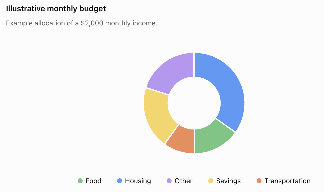
A chart makes it easier to see which categories account for the largest portions of the budget.
Reading Budget Tables
Consider this budget:
| Category | Planned | Actual |
|---|---|---|
| Food | $250 | $280 |
| Transportation | $120 | $105 |
| Entertainment | $100 | $135 |
| Clothing | $80 | $60 |
| Savings | $300 | $270 |
Tables allow us to compare what was planned with what actually happened.
Calculating Budget Differences
For food:
$280 − $250 = $30
Actual food spending was:
$30 above budget
Transportation:
$120 − $105 = $15
Actual transportation spending was:
$15 below budget
Entertainment:
$135 − $100 = $35
Actual entertainment spending was:
$35 above budget
These differences are called variances.
Interpreting Budget Data
A budget should not only be calculated. It should also be interpreted.
For example, the previous table suggests:
- food spending exceeded the planned amount by $30
- transportation spending was $15 below the planned amount
- entertainment exceeded the plan by $35
- clothing was $20 below the plan
- savings were $30 below the planned target
This information can help someone decide what adjustments to make in the next budget.
Planned vs Actual Spending
Charts can make differences easier to identify.
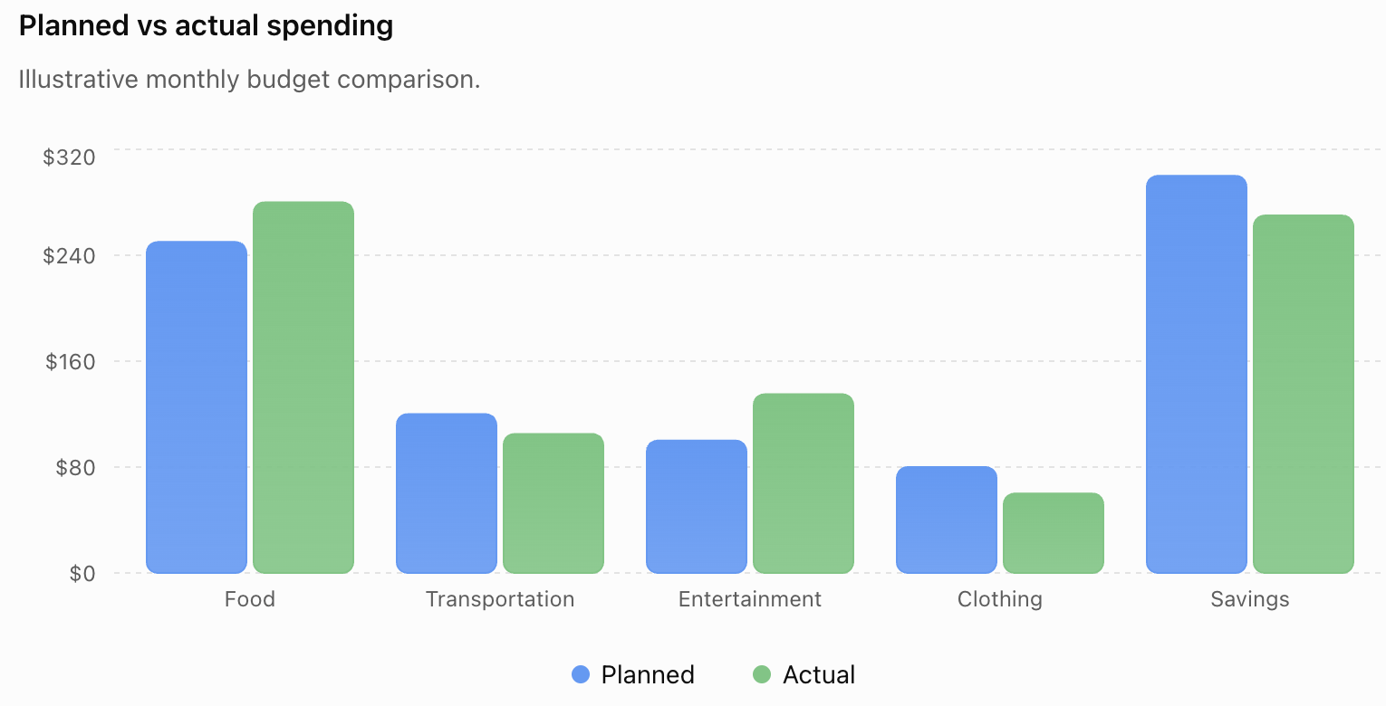
Graphs can reveal patterns that may be less obvious when looking only at individual numbers.
Comparing Financial Options
Mathematics can help compare different financial choices.
Suppose two phone plans are available.
Plan A:
$30 per month
Plan B:
$25 per month + $50 setup fee
For one month:
Plan A:
$30
Plan B:
$25 + $50 = $75
For 12 months:
Plan A:
12 × $30 = $360
Plan B:
12 × $25 + $50 = $350
The comparison changes depending on how long the service is used.


This shows why comparing only one advertised number can be misleading.
Comparing Unit Prices
Suppose:
Package A:
500 g for $4.50
Package B:
800 g for $6.40
Calculate cost per 100 g.
Package A:
500 g contains five groups of 100 g.
$4.50 ÷ 5 = $0.90 per 100 g
Package B:
800 g contains eight groups.
$6.40 ÷ 8 = $0.80 per 100 g
Unit rates make differently sized packages easier to compare.
Discounts and Budgets
Suppose an item normally costs:
$80
and is discounted by:
25%
Discount:
0.25 × $80 = $20
Sale price:
$80 − $20 = $60
If the shopping budget is $70:
$70 − $60 = $10
would remain.


Taxes and Final Prices
The displayed price is not always the final amount paid.
Suppose an illustrative purchase costs:
$120
and a tax of:
8%
is applied.
Tax:
0.08 × $120 = $9.60
Final cost:
$120 + $9.60 = $129.60
When budgeting for purchases, it is important to know whether additional charges are included in the listed price.
Tips and Service Charges
Suppose a restaurant bill is:
$60
and someone calculates a 15% tip.
Tip:
0.15 × $60 = $9
Total:
$60 + $9 = $69
In real situations, whether a tip or service charge applies depends on local practices and the bill itself.
Recurring Expenses
Small recurring expenses can become significant over time.
Suppose a subscription costs:
$12/month
Annual cost:
$12 × 12 = $144
Three similar subscriptions would cost:
3 × $144 = $432 per year


Converting recurring costs to annual amounts can make their financial impact easier to understand.
Daily Spending Over Time
Suppose someone spends:
$5 each school day
on an optional purchase.
Over 5 days:
$5 × 5 = $25
Over 20 school days:
$5 × 20 = $100
Over 180 school days:
$5 × 180 = $900
A relatively small repeated expense can become a much larger total over time.
Saving Toward a Goal
Suppose someone wants to save:
$1,200
and can save:
$150 per month
Calculate:
$1,200 ÷ $150 = 8
It would take:
8 months
assuming the same amount is saved each month.


Working Backwards from a Savings Goal
Suppose someone wants to save:
$2,400 in 12 months
Required monthly savings:
$2,400 ÷ 12 = $200
Therefore:
$200 per month
must be set aside on average.
If monthly income is $1,600:
$200 / $1,600 × 100% = 12.5%
The savings goal represents:
12.5% of monthly income
Emergency and Unexpected Expenses
Real budgets do not always follow the plan exactly.
Unexpected expenses can include:
- repairs
- replacement items
- medical or dental costs
- transportation problems
- urgent travel
- sudden changes in regular expenses
One way budgets can account for uncertainty is by including money for unexpected expenses or maintaining savings that are not already committed elsewhere.
The appropriate amount depends on the person's circumstances.
Comparing Short-Term and Long-Term Costs
Suppose:
Option A costs:
$20 per month
Option B costs:
$180 per year
Compare annual costs.
Option A:
$20 × 12 = $240/year
Option B:
$180/year
Comparing both options over the same time period provides a meaningful mathematical comparison.
The Cheapest Option Is Not Always the Best Decision
Cost is important, but financial decisions can involve more than price.
Other factors might include:
- quality
- reliability
- how long the product will last
- maintenance costs
- cancellation fees
- warranties
- convenience
- amount actually needed
For example, buying a larger package because it has a lower unit price may not save money if much of the product is wasted.
Mathematics provides evidence for a decision, but the context determines which factors matter.
Advertising and Financial Decisions
Advertisements often emphasize numbers such as:
50% OFF
Only $10/month
Buy 2, Get 1 Free
Save $100
These numbers can be useful, but they should be interpreted carefully.

Useful questions include:
- What was the original price?
- What is the final price?
- Are there additional fees?
- How long does the offer last?
- Is a subscription required?
- How much will it cost over a full year?
- How much of the product is actually needed?
Comparing Two Discounts
Store A offers:
20% off a $100 item
Discount:
$20
Final price:
$80
Store B sells the same item for:
$85 with a $10 coupon
Final price:
$75
The percentage advertised does not by itself determine the final cost.
Calculate the actual amount paid.
Using Percentages to Analyze Spending
Suppose monthly income is:
$2,400
and food spending is:
$480
Percentage of income spent on food:
480 / 2400 × 100%
= 20%
If transportation costs:
$240
then:
240 / 2400 × 100% = 10%
Percentages make categories easier to compare.
Comparing Spending Categories
Suppose someone spends:
Food = $500
Housing = $900
Transportation = $250
Entertainment = $150
Savings = $200
Total:
$2,000
Housing percentage:
900 / 2000 × 100% = 45%
Food percentage:
500 / 2000 × 100% = 25%
Transportation percentage:
12.5%
Entertainment percentage:
7.5%
Savings percentage:
10%
These percentages show how the total is distributed.


Financial Information in Tables
Suppose three savings plans are presented:
| Plan | Monthly Contribution | Annual Contribution |
|---|---|---|
| A | $50 | $600 |
| B | $75 | $900 |
| C | $100 | $1,200 |
A table helps us identify patterns and compare values quickly.
For example:
Plan C saves:
$1,200 − $600 = $600
more per year than Plan A.
But it also requires:
$50 more each month
The numbers describe the trade-off.
Financial Information in Graphs
Suppose a person's spending changes over several months.
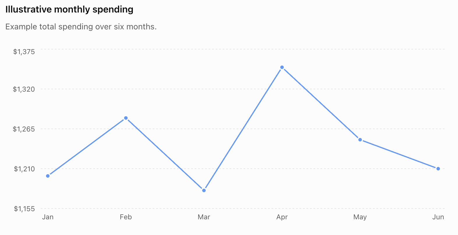
A graph can help identify:
- increases
- decreases
- unusually high months
- unusually low months
- overall patterns
However, the graph should be interpreted together with the actual values and context.
Checking Graph Scales
Graphs can sometimes make differences appear larger or smaller depending on the scale used.
Suppose two expenses are:
$100 and $105
The difference is only:
$5
If a graph's vertical axis begins at $99 instead of $0, the visual difference may appear very large.


When interpreting financial graphs, always check:
- axis labels
- units
- scale
- time period
- categories
- whether the graph begins at zero when relevant
- whether important information has been omitted
Percent Change in Expenses
Suppose an electricity bill increases from:
$80 to $100
Change:
$100 − $80 = $20
Percentage increase:
20 / 80 × 100% = 25%
Therefore:
the expense increased by 25%
Percentage changes can help compare increases involving different starting amounts.
Comparing Changes
Expense A increases:
$20 → $30
Increase:
$10
Percentage increase:
10 / 20 × 100% = 50%
Expense B increases:
$100 → $120
Increase:
$20
Percentage increase:
20 / 100 × 100% = 20%
Expense B increased by more dollars, but Expense A had the larger percentage increase.
This demonstrates why both absolute and percentage changes can be useful.
Making Decisions with Numerical Data
Suppose you have:
$500
available for a purchase.
Option A:
Purchase price = $420
Expected additional cost = $30
Total:
$450
Money remaining:
$50
Option B:
Purchase price = $390
Expected additional cost = $90
Total:
$480
Money remaining:
$20
Looking only at the purchase price would make Option B appear less expensive.
Calculating the total cost changes the comparison.
Opportunity Cost
Financial choices often involve opportunity cost.
Opportunity cost is the value of what is given up when one option is chosen instead of another.
Suppose someone has:
$100
They could spend $100 on entertainment or save the $100 toward a future goal.
If they spend it, the opportunity cost includes the savings they could have kept.
Opportunity cost is not always a simple dollar calculation, but numerical information can help make the trade-off clearer.
Budget Constraints
A constraint is a limit or condition.
Suppose you have:
$300
to organize an event.
Possible costs:
Food = $140
Decorations = $60
Equipment = $75
Total:
$140 + $60 + $75 = $275
Money remaining:
$300 − $275 = $25
The $300 budget acts as a constraint.
Any plan costing more than $300 would exceed the available budget.
Worked Example 1: Monthly Budget
Income:
$1,800
Expenses:
Housing = $650
Food = $300
Transportation = $180
Phone = $50
Entertainment = $120
Other = $100
Total expenses:
650 + 300 + 180 + 50 + 120 + 100
= $1,400
Remaining:
$1,800 − $1,400 = $400
Answer:
$400 remains
Worked Example 2: Savings
Income:
$2,500
Savings goal:
18% of income
Calculate:
0.18 × $2,500 = $450
Answer:
$450
If other expenses total $1,850:
$2,500 − $450 − $1,850 = $200
remains after savings and expenses.
Worked Example 3: Comparing Offers
Option A:
$15/month for 12 months
Total:
15 × 12 = $180
Option B:
$120 for the first 6 months + $12/month for the next 6 months
Total:
$120 + (6 × $12)
= $192
Comparing total costs over the same 12-month period provides a consistent basis for comparison.
Worked Example 4: Discount
A backpack costs:
$75
Discount:
20%
Discount amount:
0.20 × $75 = $15
Sale price:
$75 − $15 = $60
If the budget is $70:
$70 − $60 = $10
remains.
Worked Example 5: Spending Percentage
Monthly income:
$3,000
Housing:
$1,050
Percentage:
1050 / 3000 × 100%
= 35%
Therefore:
35% of income is allocated to housing
in this example.
Worked Example 6: Savings Goal
Goal:
$900
Current savings:
$300
Still needed:
$900 − $300 = $600
If $75 is saved each month:
600 ÷ 75 = 8 months
Answer:
8 additional months
assuming the saving rate remains constant.
Worked Example 7: Budget Adjustment
Income:
$1,500
Expenses:
$1,620
Deficit:
$1,620 − $1,500 = $120
To balance the budget, the person would need some combination of:
- reducing planned expenses by $120
- increasing income by $120
- or making changes totaling $120
The mathematics identifies the size of the gap.
Worked Example 8: Unit Price
Package A:
12 items for $18
Unit price:
18 ÷ 12 = $1.50/item
Package B:
20 items for $28
Unit price:
28 ÷ 20 = $1.40/item
The unit prices are:
$1.50/item versus $1.40/item
Other factors such as how many items are actually needed may also matter.
Worked Example 9: Annual Cost
A service costs:
$8.99/month
Approximate annual cost:
$8.99 × 12 = $107.88
A monthly price that appears small can therefore represent a much larger annual expense.
Worked Example 10: Multi-Step Purchase
A device costs:
$500
Discount:
15%
Discount amount:
0.15 × $500 = $75
Discounted price:
$500 − $75 = $425
Suppose an illustrative 8% tax is then applied:
0.08 × $425 = $34
Final price:
$425 + $34 = $459
Notice that the tax was calculated on the discounted price in this example.
Estimation and Financial Decisions
Estimation is useful when checking financial calculations.
Suppose:
18% of $498
is needed.
Estimate:
20% of $500 ≈ $100
Exact calculation:
0.18 × 498 = $89.64
The exact value is reasonably close to the estimate.
If a calculator produced:
$896.40
we would know something was probably wrong.


A Budget Is a Model
A budget is not a prediction that every expense will occur exactly as planned.
It is a mathematical model of expected income and spending.
Actual values can change.
For this reason, useful budgeting involves comparing:
planned values
with:
actual values
and then updating future plans.
A Reliable Financial Problem-Solving Strategy
When solving a budgeting or money problem:
Step 1: Identify the financial goal or question.
Step 2: Identify the relevant income, costs, percentages, and time periods.
Step 3: Make sure values are being compared over the same period.
Step 4: Calculate total income.
Step 5: Calculate relevant expenses.
Step 6: Find unit rates, percentages, or total costs when needed.
Step 7: Compare the numerical results.
Step 8: Check whether the answer fits the budget constraint.
Step 9: Estimate to check reasonableness.
Step 10: Explain what the numbers show before making a decision.
Common Mistakes
Mistake 1: Comparing monthly and annual costs directly
Convert them to the same time period first.
Mistake 2: Looking only at the advertised price
Additional fees, taxes, recurring charges, or required purchases may affect total cost.
Mistake 3: Confusing a discount with the final price
A $20 discount does not mean the item costs $20.
Mistake 4: Ignoring recurring costs
A small monthly expense can become significant over a year.
Mistake 5: Assuming the lowest unit price always means the lowest total spending
A larger package may have a lower unit price but require spending more money overall.
Mistake 6: Forgetting the original value when calculating percentage change
Use:
percentage change = change / original value × 100%
Mistake 7: Treating planned spending as actual spending
Budgets are plans. Actual spending should be recorded and compared with the plan.
Mistake 8: Ignoring graph scales
Always examine labels, units, intervals, and the range shown.
Did You Know?
Budgeting combines many mathematical skills rather than being a completely separate type of mathematics.


Budgeting can involve:
- addition and subtraction
- multiplication and division
- decimals
- fractions
- percentages
- ratios
- unit rates
- proportions
- tables
- graphs
- estimation
- data analysis
This makes budgeting an important real-world application of many mathematical ideas.
Key Terms
- Budget: Plan for income, spending, and saving.
- Income: Money received.
- Expense: Money spent.
- Fixed expense: Expense that generally remains constant over a particular period.
- Variable expense: Expense that can change.
- Savings: Money kept for future use rather than currently spent.
- Savings rate: Savings expressed as a percentage of income.
- Surplus: Amount by which income exceeds expenses.
- Deficit: Amount by which expenses exceed income.
- Balance: Amount remaining after expenses are subtracted from income.
- Budget constraint: Limit on how much money is available.
- Unit price: Cost for one item or one standard unit.
- Discount: Reduction from an original price.
- Tax: Amount added or collected according to an applicable tax system.
- Recurring expense: Expense that occurs repeatedly.
- Variance: Difference between a planned amount and an actual amount.
- Opportunity cost: Value of an alternative given up when a choice is made.
- Percentage change: Change expressed relative to the original amount.
Key Equations
Budget balance:
Balance = Income − Expenses
Savings rate:
Savings rate = Savings / Income × 100%
Percentage of income spent:
Spending percentage = Expense / Income × 100%
Unit price:
Unit price = Total cost / Quantity
Discount amount:
Discount = Original price × Discount rate
Sale price:
Sale price = Original price − Discount
Percentage change:
Percentage change = Change / Original value × 100%
Key Takeaways
- A budget is a mathematical plan for managing income, expenses, and savings.
- Income is money received, while expenses are money spent.
- When income exceeds expenses, there is a surplus.
- When expenses exceed income, there is a deficit.
- Savings can be expressed as an amount or as a percentage of income.
- Fixed and variable expenses behave differently and can affect how easily a budget can be adjusted.
- Tables help organize financial information.
- Charts help reveal patterns and differences in spending.
- Planned and actual spending should be compared.
- Unit prices allow products of different sizes to be compared.
- Monthly and annual costs should be converted to the same time period before comparison.
- Discounts, taxes, fees, and recurring costs can affect the final amount paid.
- Percentage calculations can show how much of income is spent or saved.
- Percentage change helps compare increases and decreases.
- Advertised prices should be interpreted in the context of total cost.
- The least expensive option is not automatically the most appropriate option because quality, quantity, reliability, and other constraints may matter.
- Estimation helps identify unreasonable calculations.
- A budget is a model and may need to change when actual income or expenses change.
- Numerical data can clarify trade-offs and consequences.
- Financial mathematics does not make a decision for us; it provides evidence that helps us understand the available options.
2. Discounts and Sales
Learning outcomes
- I can calculate discounts using percentages.
- I can determine the final price after a discount.
- I can compare multiple sale offers.
- I can calculate savings from discounts.
- I can evaluate whether a sale represents good value.


What Is a Discount?
A discount is a reduction in the original price of a product or service.
Stores often advertise discounts using percentages:
10% off
25% off
40% off
50% off
The percentage tells us what fraction of the original price will be removed.
For example:
25% off
means that 25% of the original price is subtracted.
The customer therefore pays:
75% of the original price
because:
100% − 25% = 75%
Original Price, Discount, and Sale Price
There are three important quantities in a discount problem.
Original price: Price before the discount.
Discount amount: Amount removed from the original price.
Sale price: Price after the discount has been removed.
The basic relationship is:
Sale Price = Original Price − Discount Amount
For example:
Original price = $80
Discount = $20
Sale price:
$80 − $20 = $60
Calculating a Percentage Discount
To calculate a discount:
Discount Amount = Original Price × Discount Rate
Remember to convert the percentage to a decimal.
For example:
20% = 0.20
Suppose an item costs:
$50
with:
20% off
Calculate:
$50 × 0.20 = $10
Discount:
$10
Finding the Final Price
Once we know the discount:
Sale Price = Original Price − Discount
For the previous example:
Original price:
$50
Discount:
$10
Therefore:
$50 − $10 = $40
Final price:
$40
Example: 30% Discount
A jacket originally costs:
$120
It is discounted by:
30%
Step 1: Convert the percentage.
30% = 0.30
Step 2: Calculate the discount.
$120 × 0.30 = $36
Step 3: Subtract the discount.
$120 − $36 = $84
Therefore:
Discount = $36
Final price = $84

Using Fractions for Familiar Discounts
Some percentages are easy to calculate as fractions.
50% = 1/2
25% = 1/4
75% = 3/4
20% = 1/5
10% = 1/10
For example:
25% off $80
Since:
25% = 1/4
calculate:
$80 ÷ 4 = $20
Discount:
$20
Sale price:
$80 − $20 = $60
Using Benchmark Percentages
Some discounts can be calculated mentally by combining familiar percentages.
For example:
15% = 10% + 5%
Find 15% of $60.
10%:
$60 ÷ 10 = $6
5%:
$6 ÷ 2 = $3
Therefore:
15% of $60 = $9
Sale price:
$60 − $9 = $51
Another Mental Strategy
Find:
35% of $200
We can use:
30% + 5%
30%:
$60
5%:
$10
Therefore:
35% = $70
If this is a discount:
$200 − $70 = $130
Using a Sale-Price Multiplier
There is a faster way to calculate the final price.
If an item is:
20% off
then the customer pays:
100% − 20% = 80%
Convert:
80% = 0.80
Therefore:
Sale Price = Original Price × 0.80
Example:
$150 × 0.80 = $120


Discount Multipliers
Some useful examples are:
| Discount | Percentage Paid | Multiplier |
|---|---|---|
| 10% | 90% | 0.90 |
| 15% | 85% | 0.85 |
| 20% | 80% | 0.80 |
| 25% | 75% | 0.75 |
| 30% | 70% | 0.70 |
| 40% | 60% | 0.60 |
| 50% | 50% | 0.50 |
For a 35% discount:
100% − 35% = 65%
Therefore, multiply the original price by:
0.65
Example Using a Multiplier
Original price:
$240
Discount:
35%
Percentage paid:
65%
Calculate:
$240 × 0.65 = $156
Therefore:
Final price = $156
Savings:
$240 − $156 = $84
Calculating Savings
The savings from a discount are normally equal to the discount amount.
Suppose:
Original price = $90
Discount = 20%
Calculate:
$90 × 0.20 = $18
Therefore:
Savings = $18
Final price:
$90 − $18 = $72
Discount Amount vs Final Price
These are easy to confuse.
Suppose:
Original price = $200
Discount = 30%
Discount amount:
$200 × 0.30 = $60
But the final price is:
$200 − $60 = $140
Therefore:
Savings = $60
Price paid = $140


Comparing Sale Offers
Advertisements may present discounts in different ways.
For example:
Store A: 25% off
Store B: $20 off
Which gives the larger saving?
The answer depends on the original price.
Suppose the item costs:
$100
Store A:
25% of $100 = $25
Store B:
$20
So the savings are:
$25 versus $20
What If the Original Price Is $60?
Store A:
25% of $60 = $15
Store B:
$20 off
Now the savings are:
$15 versus $20
The comparison has changed.
This demonstrates why a percentage discount cannot always be compared with a fixed discount without knowing the original price.
Finding the Break-Even Price
Suppose one offer is:
20% off
and another is:
$15 off
At what original price are the savings equal?
Let the original price be:
P
Then:
20% of P = $15
0.20P = 15
Divide:
P = 15 ÷ 0.20
P = $75
At an original price of $75, both offers save:
$15
Below or above this price, the comparison changes.
Comparing Discounts on Different Original Prices
Suppose:
Store A:
$80 shirt with 25% off
Store B:
$70 shirt with 15% off
Store A:
Discount:
$80 × 0.25 = $20
Final price:
$60
Store B:
Discount:
$70 × 0.15 = $10.50
Final price:
$59.50
A larger percentage discount does not automatically produce a lower final price because the original prices may differ.


Multiple Discounts
Stores sometimes advertise offers such as:
20% off, then an additional 10% off
It may be tempting to say:
20% + 10% = 30%
But successive discounts are normally calculated one after another.
Suppose the original price is:
$100
First discount:
20% of $100 = $20
New price:
$80
Second discount:
10% of $80 = $8
Final price:
$72
Total savings:
$100 − $72 = $28
Therefore, the total effective discount is:
28%
not 30%.
Why Successive Discounts Do Not Simply Add
After the first discount, the second percentage is applied to a smaller price.
For:
20% off, then 10% off
the multipliers are:
0.80 × 0.90
= 0.72
The customer pays:
72%
of the original price.
Therefore, the effective discount is:
28%


Another Multiple-Discount Example
Original price:
$200
Sale:
30% off, then another 20% off
First discount:
$200 × 0.70 = $140
Second discount:
$140 × 0.80 = $112
Final price:
$112
Savings:
$200 − $112 = $88
Effective discount:
$88 / $200 × 100% = 44%
So:
30% off followed by 20% off = 44% effective discount
not 50%.
Comparing One Discount with Multiple Discounts
Offer A:
40% off
Offer B:
25% off, then another 20% off
Suppose the original price is $100.
Offer A:
$100 × 0.60 = $60
Offer B:
$100 × 0.75 × 0.80 = $60
In this case, both produce the same final price.
The effective discount for Offer B is therefore also:
40%
Buy One, Get One Free
Another common sale is:
Buy One, Get One Free
Suppose each item normally costs:
$30
Two items normally cost:
$60
Under the offer:
$30
is paid for two items.
Average cost per item:
$30 ÷ 2 = $15
Compared with buying two identical items at the normal price, this is equivalent to a:
50% reduction in the total price of the two-item purchase
provided the customer actually needs two items and both qualify.


Buy Two, Get One Free
Suppose each item costs:
$12
Normally, three items cost:
3 × $12 = $36
Under:
Buy 2, Get 1 Free
the customer pays:
2 × $12 = $24
Savings:
$36 − $24 = $12
Percentage saving across the three-item bundle:
12 / 36 × 100%
= 33.3%
approximately.
Percentage Off vs Extra Product
Suppose two packages normally contain 500 g.
Offer A:
20% off the price
Offer B:
20% extra product for the same price
These offers are not mathematically identical.
If the normal price is $10:
Offer A:
500 g for:
$8
Cost per 100 g:
$8 ÷ 5 = $1.60
Offer B:
20% extra of 500 g:
0.20 × 500 = 100 g
New quantity:
600 g
Cost per 100 g:
$10 ÷ 6 ≈ $1.67
Unit rates allow the offers to be compared consistently.
Unit Price and Sales
A sale price does not automatically mean good value compared with other products.
Suppose:
Brand A:
750 g for $6 after discount.
Brand B:
1 kg for $7.50 at regular price.
Brand A:
$6 ÷ 0.75 = $8/kg
Brand B:
$7.50 ÷ 1 = $7.50/kg
The word sale alone does not tell us which option has the lower unit price.
What Does "Good Value" Mean?
Evaluating value requires more than identifying the largest discount percentage.
Mathematical information that may matter includes:
- original price
- final price
- discount amount
- quantity received
- unit price
- number of items required
- additional fees
- total cost over time
Other practical considerations can include:
- quality
- durability
- usefulness
- whether the item is actually needed
- whether some of the quantity will be wasted
Mathematics helps provide the evidence needed to evaluate the options.
Sale Price vs Value
Suppose:
Option A:
10 pens for $8
Option B:
20 pens for $14
Unit prices:
Option A:
$8 ÷ 10 = $0.80/pen
Option B:
$14 ÷ 20 = $0.70/pen
Option B has the lower unit price.
However, someone who needs only 5 pens would still have to spend:
$14
to receive that unit price.
"Better unit value" and "lower total spending" are not always the same thing.
Discounts and Budgets
Suppose your budget is:
$100
An item originally costs:
$125
It is:
25% off
Discount:
$125 × 0.25 = $31.25
Final price:
$125 − $31.25 = $93.75
Money remaining:
$100 − $93.75 = $6.25
The sale brings the item within the $100 budget.
What Percentage Was Saved?
Sometimes the original and sale prices are given instead of the discount percentage.
Suppose:
Original price:
$80
Sale price:
$60
Savings:
$80 − $60 = $20
Discount percentage:
$20 / $80 × 100%
= 25%
Therefore:
the discount was 25%
Another Reverse Discount Problem
Original price:
$150
Sale price:
$105
Savings:
$150 − $105 = $45
Percentage discount:
45 / 150 × 100%
= 30%
Therefore:
30% off
Finding the Original Price
Sometimes we know the final price and discount.
Suppose a jacket costs:
$72 after a 20% discount
A 20% discount means the customer pays:
80%
of the original price.
Let the original price be:
P
Then:
0.80P = 72
Therefore:
P = 72 ÷ 0.80
P = $90


Another Original-Price Example
A device costs:
$195 after a 35% discount
Percentage paid:
65%
Therefore:
0.65P = 195
Calculate:
P = 195 ÷ 0.65
P = $300
Original price:
$300
Discounts Followed by Additional Charges
A discount may not be the final calculation.
Suppose:
Original price:
$200
Discount:
25%
Discounted price:
$200 × 0.75 = $150
Suppose an illustrative 8% tax is then applied to the discounted price.
Tax:
$150 × 0.08 = $12
Final amount:
$150 + $12 = $162
The order of calculations matters.
Coupons and Percentage Discounts
Suppose a $100 item has:
20% off
and then a:
$10 coupon
After the percentage discount:
$100 × 0.80 = $80
After the coupon:
$80 − $10 = $70
Final price:
$70
However, real stores may have rules about whether coupons can be combined or the order in which discounts apply.
Always use the conditions stated in the problem or offer.
Comparing Three Sale Offers
Suppose an item normally costs:
$120
Offer A:
25% off
Final price:
$120 × 0.75 = $90
Offer B:
$35 off
Final price:
$120 − $35 = $85
Offer C:
10% off, then 15% off
First:
$120 × 0.90 = $108
Then:
$108 × 0.85 = $91.80
The final prices are:
| Offer | Final Price | Savings |
|---|---|---|
| A | $90.00 | $30.00 |
| B | $85.00 | $35.00 |
| C | $91.80 | $28.20 |
A comparison table makes the differences much easier to see.
Reading Sale Information from Tables
Suppose a store provides:
| Item | Original Price | Discount |
|---|---|---|
| Shoes | $80 | 25% |
| Jacket | $120 | 30% |
| Backpack | $60 | 15% |
| Headphones | $150 | 40% |
To interpret the table, we might calculate both the savings and final prices.
Shoes:
Savings = $20
Final = $60
Jacket:
Savings = $36
Final = $84
Backpack:
Savings = $9
Final = $51
Headphones:
Savings = $60
Final = $90
Tables allow several financial options to be compared systematically.


Interpreting Sale Graphs
A graph might show:
- original prices
- sale prices
- discount percentages
- savings
- prices at different stores
When reading a financial graph:
1. Read the title.
2. Check the axes.
3. Check the units.
4. Identify whether values show prices, percentages, or savings.
5. Compare actual numerical values rather than relying only on visual appearance.
6. Check whether the graph scale could exaggerate differences.
Sale Advertisements
Advertisements commonly use phrases such as:
UP TO 70% OFF
SAVE $50
FROM $19.99
BUY ONE, GET ONE FREE
20% EXTRA

These statements do not all mean the same thing.
For example:
"Up to 70% off"
means some qualifying items may have a 70% discount. It does not mean every item is discounted by 70%.
Careful interpretation is part of mathematical financial literacy.
Percentage Discount vs Dollar Savings
A large percentage discount does not necessarily mean a large amount of money saved.
Item A:
$20 with 50% off
Savings:
$10
Item B:
$500 with 10% off
Savings:
$50
Item A has the larger percentage discount.
Item B produces the larger dollar saving.
Which measure matters depends on the question being asked.
Original Price Matters
Compare:
50% off $20
and:
20% off $100
First:
0.50 × $20 = $10 saved
Second:
0.20 × $100 = $20 saved
The smaller percentage produces the larger dollar saving because it applies to a larger original price.
Estimating Sale Prices
Estimation can help check calculations.
Suppose:
32% off $198
Estimate:
About 30% of $200:
≈ $60
So the sale price should be roughly:
$140
Exact discount:
$198 × 0.32 = $63.36
Exact sale price:
$198 − $63.36 = $134.64
The exact answer is reasonably close to the estimate.


Checking Whether an Answer Is Reasonable
If an item is:
20% off
the final price should be:
- lower than the original price
- greater than 50% of the original price
- exactly 80% of the original price
For a $100 item:
A final price of:
$80
makes sense.
A final price of:
$20
would mean the discount amount has been confused with the sale price.
Worked Example 1: Basic Discount
Original price:
$70
Discount:
20%
Savings:
$70 × 0.20 = $14
Final price:
$70 − $14 = $56
Answer:
Savings = $14
Final price = $56
Worked Example 2: 35% Off
Original price:
$160
Discount:
35%
Savings:
$160 × 0.35 = $56
Final price:
$160 − $56 = $104
Worked Example 3: Using a Multiplier
Original price:
$280
Discount:
15%
Percentage paid:
85%
Calculate:
$280 × 0.85 = $238
Final price:
$238
Savings:
$42
Worked Example 4: Comparing Offers
A $200 item has two possible offers.
Offer A:
30% off
Savings:
$60
Final:
$140
Offer B:
$50 off
Savings:
$50
Final:
$150
The offers produce final prices of:
$140 and $150
Worked Example 5: Successive Discounts
Original price:
$250
Discounts:
20% off, then 15% off
First:
$250 × 0.80 = $200
Second:
$200 × 0.85 = $170
Final price:
$170
Savings:
$250 − $170 = $80
Effective discount:
80 / 250 × 100% = 32%
Worked Example 6: Find the Discount Percentage
Original price:
$240
Sale price:
$180
Savings:
$240 − $180 = $60
Percentage discount:
60 / 240 × 100%
= 25%
Worked Example 7: Find the Original Price
Sale price:
$126
Discount:
30%
Percentage paid:
70%
Therefore:
0.70P = 126
P = 126 ÷ 0.70
P = $180
Worked Example 8: Buy Two, Get One Free
Each shirt costs:
$24
Normally three shirts cost:
3 × $24 = $72
Under the offer:
2 × $24 = $48
Savings:
$24
Percentage saving:
24 / 72 × 100%
≈ 33.3%
Worked Example 9: Unit-Price Comparison
Offer A:
600 g for $4.80
Offer B:
900 g for $6.75
Offer A:
$4.80 ÷ 6 = $0.80 per 100 g
Offer B:
$6.75 ÷ 9 = $0.75 per 100 g
The unit prices provide a common basis for comparing the offers.
Worked Example 10: Budget and Sale
Budget:
$150
Original price:
$180
Discount:
25%
Final price:
$180 × 0.75 = $135
Money remaining:
$150 − $135 = $15
The discounted item fits within the stated budget.
Evaluating a Sale
When deciding whether a sale represents useful value, ask:
What is the original price?
What percentage is actually discounted?
How many dollars will I save?
What is the final price?
How does the unit price compare with alternatives?
Are there additional charges?
Do I need to buy more items to receive the discount?
Will I actually use the extra quantity?
Is another store's regular price lower?
Does the purchase fit the available budget?
A large discount percentage by itself does not answer all of these questions.
A Reliable Discount Strategy
Step 1: Identify the original price.
Step 2: Identify the discount percentage or offer.
Step 3: Convert the percentage to a decimal or fraction.
Step 4: Calculate the discount amount.
Step 5: Subtract the discount from the original price.
Step 6: Include any additional calculations stated in the problem.
Step 7: If comparing offers, calculate each final price on the same basis.
Step 8: Compare savings and unit prices when relevant.
Step 9: Estimate to check your calculation.
Step 10: Interpret the numbers in the context of the purchase.
Common Mistakes
Mistake 1: Treating the discount as the final price
20% off $100 means:
$20 saved
not:
$20 final price
The final price is:
$80
Mistake 2: Forgetting to convert the percentage
Incorrect:
$80 × 25
Correct:
$80 × 0.25
Mistake 3: Subtracting the percentage number directly
Incorrect:
$100 − 20 = $80
This happens to produce the correct number only because the original price is $100.
For $200:
20% off is:
$40
not $20.
Mistake 4: Adding successive discounts
20% off followed by 10% off is:
28% effective discount
not 30%.
Mistake 5: Assuming the largest percentage means the lowest price
Original prices may be different.
Mistake 6: Assuming a sale automatically means good value
Another product may have a lower regular price or lower unit price.
Mistake 7: Ignoring conditions
Some discounts require:
- buying multiple items
- spending a minimum amount
- membership
- using a coupon
- purchasing during a particular period
Mistake 8: Ignoring how much is actually needed
A lower unit price may require purchasing much more than necessary.
Did You Know?
Discount mathematics combines several mathematical ideas.


When comparing sales, we may use:
- percentages
- decimals
- fractions
- ratios
- unit rates
- proportions
- estimation
- tables
- graphs
- algebra
This is why shopping provides a useful real-world application of mathematics.
Key Terms
- Original price: Price before a discount.
- Discount: Reduction in price.
- Discount rate: Percentage by which the original price is reduced.
- Discount amount: Amount of money removed from the original price.
- Sale price: Price after the discount.
- Final price: Amount paid after the calculations specified in the problem.
- Savings: Difference between the original price and the discounted price.
- Multiplier: Decimal used to calculate a percentage of an amount directly.
- Successive discount: One discount applied after another.
- Effective discount: Overall percentage reduction produced by one or more discounts.
- Unit price: Cost per one item or standard unit of quantity.
- Coupon: Offer that reduces a price when its conditions are satisfied.
- Break-even point: Value at which two financial options produce the same result.
- Value: Relationship between what is received and what it costs.
Key Equations
Discount amount:
Discount = Original Price × Discount Rate
Sale price:
Sale Price = Original Price − Discount
Percentage paid:
Percentage Paid = 100% − Discount Percentage
Multiplier method:
Sale Price = Original Price × Percentage Paid as a Decimal
Savings:
Savings = Original Price − Sale Price
Discount percentage:
Discount % = Savings / Original Price × 100%
Original price:
Original Price = Sale Price / Percentage Paid as a Decimal
Key Takeaways
- A discount reduces the original price of a product or service.
- Percentage discounts are calculated from the original price unless the offer specifies otherwise.
- The discount amount is the amount saved, not usually the final price.
- The sale price equals the original price minus the discount.
- A multiplier can calculate a sale price directly.
- A 20% discount means paying 80% of the original price.
- Savings can be calculated in dollars or as a percentage.
- Fixed-dollar discounts and percentage discounts should be compared using actual savings or final prices.
- Different original prices can make percentage comparisons misleading.
- Successive discounts are applied one after another and normally should not simply be added.
- Unit prices are useful when sale packages contain different quantities.
- "Buy one, get one free" and similar offers should be analyzed using the total cost and quantity received.
- The largest advertised discount does not automatically produce the lowest final price.
- A lower unit price does not automatically mean lower total spending.
- Additional fees or charges may affect the final amount.
- Estimation is useful for checking discount calculations.
- Sale advertisements should be interpreted carefully, especially phrases such as "up to", "from", and "extra."
- Evaluating value requires comparing the numerical evidence with the quantity, cost, conditions, and purpose of the purchase.
- The most useful question is not simply "How big is the discount?" but:
"What will I actually pay, what will I receive, and how does that compare with the alternatives?"
3. Interest and Growth
Learning outcomes
- I can explain the concept of interest.
- I can calculate simple interest in practical situations.
- I can interpret growth expressed as percentages.
- I can compare different savings options.
- I can explain how interest affects financial decisions.


4. Probability as Fractions and Percentages
Learning outcomes
- I can express probabilities as fractions, decimals, and percentages.
- I can calculate simple probabilities.
- I can compare the likelihood of different events.
- I can interpret probability information in real-life situations.
- I can use probability to make predictions.


What Is Probability?
Probability is a measure of how likely an event is to happen.
We use probability whenever there is uncertainty about an outcome.
Examples include:
- whether a coin lands heads or tails
- which number appears when a die is rolled
- which color is selected from a bag
- whether it will rain
- whether a machine produces a defective item
- how often a particular result may occur in repeated trials
Probability does not usually tell us exactly what will happen next. Instead, it describes how likely different outcomes are.
The Probability Scale
Probability ranges from:
0 to 1
or:
0% to 100%


Important points include:
0 = 0% = impossible
1/4 = 0.25 = 25% = unlikely
1/2 = 0.5 = 50% = even chance
3/4 = 0.75 = 75% = likely
1 = 100% = certain
A probability can never be less than 0 or greater than 1.
Probability as a Fraction
When outcomes are equally likely:
Probability = Number of favorable outcomes / Total number of possible outcomes
We often write this as:
P(event) = favorable outcomes / total outcomes
For example, a fair six-sided die has six possible outcomes:
1, 2, 3, 4, 5, 6
The probability of rolling a 4 is:
P(4) = 1/6
There is one favorable outcome out of six possible outcomes.
Probability as a Decimal
A fraction can be converted to a decimal by dividing:
numerator ÷ denominator
For example:
1/4 = 1 ÷ 4 = 0.25
Therefore:
P = 0.25
Probability as a Percentage
To convert a decimal probability into a percentage:
Decimal × 100%
For example:
0.25 × 100% = 25%
Therefore:
1/4 = 0.25 = 25%
All three values describe exactly the same probability.


Common Probability Equivalents
| Fraction | Decimal | Percentage |
|---|---|---|
| 0 | 0 | 0% |
| 1/10 | 0.1 | 10% |
| 1/5 | 0.2 | 20% |
| 1/4 | 0.25 | 25% |
| 1/2 | 0.5 | 50% |
| 3/4 | 0.75 | 75% |
| 4/5 | 0.8 | 80% |
| 9/10 | 0.9 | 90% |
| 1 | 1 | 100% |
Recognizing these common equivalents makes probability comparisons much easier.
Simple Probability
Suppose a bag contains:
3 red counters
2 blue counters
5 counters altogether
What is the probability of selecting red?
Favorable outcomes:
3
Total outcomes:
5
Therefore:
P(red) = 3/5
Convert to decimal:
3 ÷ 5 = 0.6
Convert to percentage:
0.6 × 100% = 60%
Therefore:
P(red) = 3/5 = 0.6 = 60%


Probability with a Fair Coin
A fair coin has two possible outcomes:
Heads
Tails
Therefore:
P(heads) = 1/2
and:
P(tails) = 1/2
Convert:
1/2 = 0.5 = 50%
So each outcome has a 50% probability on a single fair toss.


Probability with a Fair Die
A standard fair die has six possible outcomes:
1, 2, 3, 4, 5, 6
Each individual number has probability:
1/6
What is the probability of rolling an even number?
Even numbers:
2, 4, 6
There are:
3 favorable outcomes
Therefore:
P(even) = 3/6
Simplify:
P(even) = 1/2
So:
P(even) = 0.5 = 50%
Another Die Example
What is the probability of rolling a number greater than 4?
Possible favorable outcomes:
5, 6
Therefore:
P(number > 4) = 2/6
Simplify:
1/3
Decimal:
1 ÷ 3 ≈ 0.333
Percentage:
≈ 33.3%


Probability with a Spinner
Suppose a spinner has:
8 equal sections
with:
3 red
2 blue
2 green
1 yellow
Probability of red:
3/8
Decimal:
0.375
Percentage:
37.5%
Probability of yellow:
1/8
Decimal:
0.125
Percentage:
12.5%


Because red occupies more equal sections than yellow, red is more likely to occur.
Equally Likely Outcomes
The simple formula:
P(event) = favorable outcomes / total outcomes
works directly when the individual outcomes are equally likely.
For example, with a fair die, each face has the same probability.
But suppose a spinner contains sections of different sizes.
A large section may be more likely than a small section.


In that situation, simply counting the number of sections may not correctly determine probability.
The size or probability of each outcome must also be considered.
Favorable Outcomes
A favorable outcome is an outcome that satisfies the event we are interested in.
Suppose a die is rolled.
Event:
Roll a number less than 5
Favorable outcomes:
1, 2, 3, 4
Therefore:
P(number < 5) = 4/6
Simplify:
2/3
This does not mean that 1, 2, 3, and 4 are "good." In probability, favorable simply means that the outcome matches the event being investigated.
Impossible Events
An impossible event has probability:
0
For example, rolling a 9 on a standard six-sided die is impossible.
Therefore:
P(9) = 0
or:
0%
Certain Events
A certain event has probability:
1
For example, rolling a number less than 7 on a standard six-sided die is certain.
Possible outcomes:
1, 2, 3, 4, 5, 6
All six satisfy the condition.
Therefore:
P(number < 7) = 6/6 = 1 = 100%
Likelihood Language
Probability can also be described using words.

Impossible: probability = 0
Unlikely: probability closer to 0 than 0.5
Even chance: probability = 0.5
Likely: probability closer to 1 than 0.5
Certain: probability = 1
These words describe general levels of likelihood rather than always specifying an exact probability.
Comparing Probabilities
Suppose:
Event A:
P(A) = 1/4
Event B:
P(B) = 0.40
Event C:
P(C) = 35%
Convert them to the same form.
Event A:
1/4 = 25%
Event B:
0.40 = 40%
Event C:
35%
Now the probabilities are:
A = 25%
B = 40%
C = 35%
Putting probabilities in the same form makes them much easier to compare.
Comparing Fractions
Suppose:
P(A) = 2/5
and:
P(B) = 3/8
Convert to decimals:
2/5 = 0.40
3/8 = 0.375
Therefore:
0.40 > 0.375
So event A has the greater probability.
Complementary Events
The complement of an event is the event not happening.
For any event A:
P(A) + P(not A) = 1
or:
100%
Suppose:
P(rain) = 30%
Then:
P(no rain) = 100% − 30%
= 70%


Complement Example with a Die
What is the probability of not rolling a 6?
Probability of rolling 6:
1/6
Therefore:
P(not 6) = 1 − 1/6
= 5/6
or approximately:
83.3%
Theoretical Probability
Theoretical probability is based on a mathematical model of possible outcomes.
For a fair coin:
P(heads) = 1/2
For a fair six-sided die:
P(6) = 1/6
These probabilities can be calculated before conducting an experiment.
Experimental Probability
Experimental probability is based on actual observations or trials.
The equation is:
Experimental Probability = Number of Times Event Occurs / Total Number of Trials
Suppose a coin is tossed 50 times.
Heads occurs:
27 times
Experimental probability:
27/50
= 0.54
= 54%


The theoretical probability is 50%, but an experiment does not have to produce exactly 50%.
Why Experimental Results Vary
Random processes naturally produce variation.
A fair coin tossed 10 times might produce:
7 heads and 3 tails
That does not necessarily mean:
P(heads) = 70%
The theoretical probability remains:
50%
for a fair coin.
With a larger number of trials, experimental proportions often become closer to the theoretical probability.
This idea is connected to the law of large numbers.
Relative Frequency
Experimental probability is also called relative frequency.
Suppose a basketball player takes:
80 free throws
and makes:
60
Relative frequency of success:
60/80
= 3/4
= 0.75
= 75%
This information can be used to describe past performance and may help estimate future outcomes, while recognizing that future results are uncertain.
Using Probability to Make Predictions
Probability can help estimate how many times an event may occur over many trials.
Suppose:
P(red) = 0.30
and a random selection experiment is performed:
200 times
Expected number of red outcomes:
0.30 × 200 = 60
Therefore, we might predict:
about 60 red outcomes


This is a prediction, not a guarantee.
Expected Frequency
The expected number of times an event occurs can be calculated using:
Expected Frequency = Probability × Number of Trials
For example:
Probability of success:
0.4
Number of trials:
150
Expected frequency:
0.4 × 150 = 60
We would expect approximately:
60 successes
over many similar trials.
Prediction with Fractions
Suppose:
P(blue) = 3/5
and there will be:
100 selections
Expected blue outcomes:
3/5 × 100
= 60
Prediction:
about 60 blue outcomes
Prediction with Percentages
Suppose a machine historically produces:
2% defective items
If:
5,000 items
are produced under similar conditions, a simple prediction based on that rate is:
2% of 5,000
0.02 × 5000 = 100
So the expected number is:
about 100 defective items
Actual results could be higher or lower.
Probability in Weather Information
Weather forecasts often use probabilities.
Suppose a forecast reports:
70% chance of rain
This describes a probability associated with the forecast event and its specified place and time period.


It does not mean that it will rain for exactly 70% of the day.
It also does not guarantee that rain will occur.
A probability describes uncertainty, not certainty.
Probability in Sports
Sports statistics often use past frequencies.
Suppose a player successfully completes:
42 of 60 attempts
Success rate:
42/60
Simplify:
7/10
Decimal:
0.70
Percentage:
70%
If the player makes another 100 attempts under broadly similar conditions, 70 successes might be used as a simple prediction based on the historical rate.
But actual performance can change.


Probability in Games
Games frequently involve probability.
Examples include:
- dice
- cards
- spinners
- coins
- random number generators
Suppose a game awards a prize if a player rolls a 6.
Probability of winning:
1/6
Probability of not winning:
5/6
Knowing these probabilities can help us understand how the game is structured.
Probability with Cards
A standard deck contains:
52 cards
There are:
4 suits
with:
13 cards in each suit
Probability of drawing a heart:
13/52
Simplify:
1/4
Therefore:
P = 0.25 = 25%


Another Card Example
There are four aces in a standard 52-card deck.
Therefore:
P(ace) = 4/52
Simplify:
1/13
Decimal:
≈ 0.077
Percentage:
≈ 7.7%
Probability from Tables
Suppose a survey records preferred transportation:
| Transportation | Students |
|---|---|
| Walk | 24 |
| Bus | 36 |
| Car | 20 |
| Bicycle | 20 |
Total:
24 + 36 + 20 + 20 = 100
If one student is randomly selected:
P(bus) = 36/100 = 0.36 = 36%
P(bicycle) = 20/100 = 0.20 = 20%
Tables can therefore be used to calculate probabilities from data.
Probability from Graphs
Graphs can also provide information used to estimate probabilities.
Suppose a graph shows:
Red = 40 outcomes
Blue = 30 outcomes
Green = 20 outcomes
Yellow = 10 outcomes
Total:
100 outcomes
Therefore:
P(red) = 40/100 = 40%
P(blue) = 30/100 = 30%
P(green) = 20/100 = 20%
P(yellow) = 10/100 = 10%


Interpreting Probability Data Carefully
Suppose:
20 people are surveyed.
16 choose option A.
Experimental proportion:
16/20 = 80%
It would be correct to say:
80% of the surveyed group chose A.
It would require additional assumptions to claim that exactly 80% of a much larger population would choose A.
The size and selection of the sample matter when probability and statistics are used to make predictions.
Probability Does Not Guarantee Individual Outcomes
Suppose:
P(win) = 90%
This means winning is very likely under the stated model.
It does not mean winning is certain.
A 10% probability of not winning still exists.
Similarly:
P(event) = 1%
does not mean the event is impossible.
Low probability and impossibility are different ideas.
Random Does Not Mean "Equal"
A process can be random without every outcome having the same probability.
For example, imagine a spinner where:
70% of the area is blue
and:
30% is red.
The result may still be random, but:
P(blue) = 0.70
and:
P(red) = 0.30

Independent Repeated Events
Suppose a fair coin has landed heads five times in a row.
If each toss is independent, the probability of heads on the next toss is still:
1/2
The coin does not "owe" us a tail.
Previous independent results do not change the probability of the next toss.
This common misunderstanding is sometimes called the gambler's fallacy.
Probability and Risk
Probability is often used to describe risk.
For example, suppose two hypothetical events have probabilities:
Event A:
2%
Event B:
20%
Event B is ten times as likely under the stated model:
20% ÷ 2% = 10
However, probability is only one part of evaluating risk. The consequences of an event may also matter.
Worked Example 1: Colored Counters
A bag contains:
4 red
5 blue
1 yellow
Total:
10
Probability of blue:
5/10 = 1/2
Decimal:
0.5
Percentage:
50%
Worked Example 2: Die
What is the probability of rolling a number greater than 2?
Favorable outcomes:
3, 4, 5, 6
Therefore:
P(>2) = 4/6
Simplify:
2/3
Decimal:
≈ 0.667
Percentage:
≈ 66.7%
Worked Example 3: Spinner
A spinner has 20 equal sections.
Eight are green.
Probability:
8/20
Simplify:
2/5
Decimal:
0.4
Percentage:
40%
Worked Example 4: Compare Probabilities
Event A:
3/4
Event B:
0.70
Event C:
72%
Convert:
A = 75%
B = 70%
C = 72%
So their probabilities are:
75%, 70%, and 72%
Converting to a common representation makes the comparison clear.
Worked Example 5: Complement
Probability of success:
0.65
Probability of failure:
1 − 0.65 = 0.35
Therefore:
P(failure) = 35%
Worked Example 6: Experimental Probability
A spinner is used:
200 times
Blue occurs:
46 times
Experimental probability:
46/200
= 0.23
= 23%
Worked Example 7: Prediction
Suppose:
P(success) = 35%
There will be:
400 trials
Expected successes:
0.35 × 400 = 140
Prediction:
about 140 successes
Worked Example 8: Using Historical Data
A sports player succeeds:
72 times in 90 attempts
Experimental probability:
72/90
= 0.8
= 80%
If the player makes another 50 attempts under similar conditions:
Expected successes:
0.80 × 50 = 40
A simple prediction is:
about 40 successes
This remains an estimate rather than a guarantee.
Worked Example 9: Probability from a Table
A survey gives:
| Choice | Frequency |
|---|---|
| A | 45 |
| B | 30 |
| C | 15 |
| D | 10 |
Total:
100
If one response is randomly selected:
P(A) = 45%
P(B) = 30%
P(C) = 15%
P(D) = 10%
Worked Example 10: Multi-Step Probability
A bag contains:
6 red
3 blue
1 green
Total:
10
Probability of selecting something that is not red:
Blue or green outcomes:
3 + 1 = 4
Therefore:
P(not red) = 4/10
= 2/5
= 0.4
= 40%
We could also use the complement:
P(red) = 6/10 = 60%
Therefore:
P(not red) = 100% − 60% = 40%
Making Predictions from Probability
Probability-based predictions are most useful over many trials.
Suppose:
P(A) = 0.25
For 20 trials:
Expected frequency:
0.25 × 20 = 5
For 100 trials:
0.25 × 100 = 25
For 1,000 trials:
0.25 × 1000 = 250


The actual results may differ from these numbers, especially for smaller numbers of trials.
A Reliable Probability Strategy
Step 1: Identify the event.
What exactly are you trying to find?
Step 2: Identify all possible outcomes.
Step 3: Determine whether the outcomes are equally likely.
Step 4: Count the favorable outcomes.
Step 5: Calculate:
P(event) = favorable outcomes / total outcomes
Step 6: Simplify the fraction if possible.
Step 7: Convert to a decimal or percentage if required.
Step 8: Check that the probability is between 0 and 1.
Step 9: Interpret what the probability means in context.
Step 10: If making a prediction, remember that expected results are not guaranteed results.
Common Mistakes
Mistake 1: Writing a probability greater than 1
For example:
P(A) = 1.4
cannot be a valid probability.
Mistake 2: Forgetting the total number of outcomes
If a bag contains 3 red and 7 blue counters:
P(red) = 3/10
not:
3/7
Mistake 3: Confusing percentages and decimals
25% = 0.25
not:
25
Mistake 4: Assuming all outcomes are equally likely
This is only valid when the model supports that assumption.
Mistake 5: Treating a prediction as a guarantee
A predicted 60 successes does not mean exactly 60 must occur.
Mistake 6: Treating unlikely as impossible
A probability of 1% is small, but it is not zero.
Mistake 7: Treating likely as certain
A probability of 90% is high, but it is not 100%.
Mistake 8: Assuming short experiments must match theoretical probability
Ten fair coin tosses do not have to produce exactly five heads.
Mistake 9: Assuming previous independent results control the next result
Five heads in a row do not make tails "due" on the next independent toss.
Did You Know?
Probability connects many areas of mathematics and real-world decision-making.


Probability is used in:
- weather forecasting
- science
- genetics
- medicine and public health research
- engineering
- manufacturing
- sports statistics
- insurance
- economics
- quality control
- computer science
- games
In each case, probability helps describe uncertainty.
Key Terms
- Probability: Measure of how likely an event is.
- Outcome: One possible result.
- Event: One outcome or a collection of outcomes being investigated.
- Favorable outcome: Outcome that satisfies the event being studied.
- Equally likely: Outcomes having the same probability.
- Impossible event: Event with probability 0.
- Certain event: Event with probability 1.
- Likelihood: How probable an event is.
- Complement: Event consisting of an event not occurring.
- Theoretical probability: Probability calculated from a mathematical model.
- Experimental probability: Probability estimated from observed results.
- Relative frequency: Proportion of trials in which an event occurs.
- Trial: One performance of a probability experiment.
- Expected frequency: Predicted number of occurrences based on probability.
- Random: Involving uncertainty in individual outcomes.
- Independent events: Events where the outcome of one does not affect the probability of another.
- Prediction: Estimate of future results based on available information.
Key Equations and Rules
Simple probability for equally likely outcomes:
P(event) = Favorable Outcomes / Total Possible Outcomes
Experimental probability:
P(event) = Number of Times Event Occurs / Total Number of Trials
Complement rule:
P(A) + P(not A) = 1
Therefore:
P(not A) = 1 − P(A)
Expected frequency:
Expected Frequency = Probability × Number of Trials
Fraction to decimal:
Numerator ÷ Denominator
Decimal to percentage:
Decimal × 100%
Percentage to decimal:
Percentage ÷ 100
Key Takeaways
- Probability measures how likely an event is to occur.
- Probabilities range from 0 to 1, or from 0% to 100%.
- A probability of 0 represents an impossible event.
- A probability of 1 represents a certain event.
- An even chance has probability 1/2 = 0.5 = 50%.
- Probabilities can be written as fractions, decimals, or percentages.
- Different forms can represent exactly the same probability.
- For equally likely outcomes, probability can be calculated using favorable outcomes divided by total possible outcomes.
- Probabilities are easier to compare when converted to the same form.
- Complementary probabilities add to 1, or 100%.
- Theoretical probability comes from a mathematical model.
- Experimental probability comes from observed data.
- Experimental results may differ from theoretical probabilities.
- Larger numbers of trials often produce experimental proportions closer to theoretical probabilities.
- Expected frequency can be calculated by multiplying probability by the number of trials.
- Probability can be used to make predictions, but predictions are not guarantees.
- Random does not necessarily mean that all outcomes are equally likely.
- Past independent outcomes do not make a particular future outcome "due."
- Real-world probability information should be interpreted in context, especially when it comes from samples or historical data.
- Probability is useful because it gives us a mathematical way to describe and reason about uncertainty.
5. Review and Real-World Projects
Learning outcomes
- I can apply fractions, ratios, decimals, and percentages to solve complex problems.
- I can choose appropriate mathematical strategies for practical situations.
- I can interpret and analyze real-world numerical information.
- I can communicate my mathematical thinking clearly.
- I can complete projects that demonstrate the usefulness of mathematics in everyday life.


