Advanced Applications and Mathematical Connections

Introduction

Vectors and matrices are among the most powerful tools in mathematics because they allow us to represent, analyse, and solve problems involving several quantities simultaneously.

Throughout this course, we have explored how vectors describe magnitude and direction, how matrices represent transformations and systems of equations, and how linear algebra supports applications in science, engineering, computer graphics, data science, and artificial intelligence.

However, real-world mathematical problems rarely require just one isolated technique.

A navigation problem might combine vector addition, trigonometry, and simultaneous equations. An engineering problem might involve matrices, forces, and equilibrium conditions. A computer graphics problem may require several transformations applied in a particular order. A data science problem may combine matrix multiplication, regression, and optimisation.

Comprehensive problem solving involves recognising these connections and selecting the most appropriate mathematical tools.

In this lesson, we will integrate the major concepts from vectors and matrices, develop systematic problem-solving strategies, examine challenging multi-step applications, and practise communicating complete mathematical solutions.

The Mathematical Problem-Solving Process

Complex mathematical problems become more manageable when approached systematically.

A useful strategy involves six stages.

This process is particularly important when a problem requires several different mathematical ideas.

Reviewing the Main Tools of Linear Algebra

Before solving integrated problems, we should recognise the major mathematical techniques available.

The key skill is not simply remembering these techniques. It is recognising which technique is appropriate and why.

Choosing an Efficient Mathematical Method

Different mathematical problems suggest different approaches.

A good mathematician selects a method based on the structure of the problem rather than applying the same procedure to every situation.

Integrated Problem 1: Navigation Using Vectors

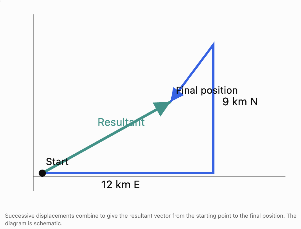
A rescue boat travels 12 km east and then 9 km north.

A current subsequently causes an additional displacement of 3 km west and 4 km south.

Determine the boat's final displacement from its starting position.

Step 1: Choose a Coordinate System

Let:

• East be the positive x-direction.

• North be the positive y-direction.

The first displacement is:

The second displacement is:

The current produces:

Step 2: Add the Displacement Vectors

The boat finishes 9 km east and 5 km north of its starting position.

Step 3: Calculate the Magnitude

Step 4: Calculate the Direction

The direction is 29.1° north of east.

Final Answer

The resultant displacement is approximately 10.30 km at 29.1° north of east.

Verification

The horizontal displacement is:

12 − 3 = 9 km east.

The vertical displacement is:

9 − 4 = 5 km north.

Both components agree with the resultant vector.

Integrated Problem 2: Forces and Equilibrium

A sign with weight 120 N hangs from two cables.

The left cable makes an angle of 30° above the horizontal.

The right cable makes an angle of 60° above the horizontal.

Determine the tension in each cable.

Step 1: Define the Unknowns

Let:

T₁ = tension in the left cable.

T₂ = tension in the right cable.

The sign is stationary, so the net force is zero.

Step 2: Resolve Horizontal Forces

The horizontal components must balance:

Therefore:

Multiplying by 2:

Step 3: Resolve Vertical Forces

The upward forces must balance the weight:

Therefore:

Multiplying by 2:

Step 4: Express as a Matrix Equation

Step 5: Solve the System

From the first equation:

Substitute:

Then:

Step 6: Verify

Horizontal components:

Vertical components:

Both equilibrium conditions are satisfied.

Interpretation

The right cable has greater tension because it provides a larger share of the upward force.

This problem integrates vector resolution, trigonometry, matrix representation, and simultaneous equations.

Integrated Problem 3: Solving an Engineering System

An electrical network is modelled by three simultaneous equations:

where I₁, I₂, and I₃ are currents measured in amperes.

Find the three currents.

Step 1: Construct the Matrix Equation

where:

Step 2: Use Substitution or Elimination

From the first equation:

From the third:

Therefore:

Substitute into the middle equation:

Using I₂ = 3I₃ − 5:

Then:

And:

Final Answer

Approximately:

I₁ = 3.13 A

I₂ = 2.40 A

I₃ = 2.47 A

Verification

First equation:

Second equation:

Third equation:

All equations are satisfied.

Integrated Problem 4: Determinants and Inverse Matrices

Consider the matrix:

We want to determine whether A is invertible and use it to solve:

Step 1: Calculate the Determinant

For a 2 × 2 matrix:

Therefore:

Since the determinant is nonzero, A is invertible.

Step 2: Find the Inverse

Step 3: Solve

Step 4: Verify

The solution is correct.

Choosing an Efficient Method

For a single system, Gaussian elimination is often more efficient than calculating the inverse explicitly.

However, the inverse is useful when investigating the transformation itself or when studying how solutions depend on different right-hand-side vectors.

Integrated Problem 5: Geometric Transformations

A triangle has vertices:

A(1, 1)

B(3, 1)

C(2, 3)

It undergoes the following transformations:

1. Reflection in the y-axis.

2. Rotation of 90° anticlockwise about the origin.

3. Enlargement by scale factor 2.

Determine the final coordinates.

Step 1: Reflection Matrix

Reflection in the y-axis:

Step 2: Rotation Matrix

A 90° anticlockwise rotation:

Step 3: Enlargement Matrix

Scale factor 2:

Step 4: Combine the Transformations

The transformations are applied in the order:

Reflection, rotation, enlargement.

Therefore:

First:

Then:

Step 5: Transform Each Vertex

For any point:

Therefore:

For A(1, 1):

A′(−2, −2)

For B(3, 1):

B′(−2, −6)

For C(2, 3):

C′(−6, −4)

Final Answer

Step 6: Verify Using the Determinant

The absolute determinant is 4.

Therefore, areas are multiplied by 4.

The negative sign indicates a reversal of orientation.

This is consistent with the reflection.

Integrated Problem 6: Eigenvalues and Long-Term Behaviour

Consider a system described by:

where:

The matrix represents movement between two categories.

Each column sums to 1, so A is a column-stochastic transition matrix.

Suppose:

Step 1: Calculate the First State

Step 2: Calculate the Second State

Step 3: Find the Steady State

A steady-state vector satisfies:

Therefore:

Let:

Then:

Therefore:

The total population is 100:

Final Answer

The system approaches a steady-state distribution of 60 in the first category and 40 in the second.

Interpretation

The steady-state vector is an eigenvector associated with eigenvalue 1.

The other eigenvalue is 0.5, so deviations from the steady state decrease over time.

This connects matrix multiplication, eigenvalues, eigenvectors, and mathematical modelling.

Integrated Problem 7: Data Science and Least Squares

A scientist measures how a quantity y changes with x.

The observations are:

The scientist wants to fit a linear model:

Step 1: Construct the Design Matrix

The parameter vector is:

The observation vector is:

Step 2: Form the Normal Equations

Calculate:

and:

Therefore:

Step 3: Solve

The equations are:

Multiply the second equation by 2:

Subtract:

Then:

Final Model

Step 4: Verify

For x = 1:

y = 3

For x = 2:

y = 5

For x = 3:

y = 7

All observations lie exactly on the fitted line.

The residuals are all zero.

Therefore:

This example integrates matrices, simultaneous equations, and statistical modelling.

Integrated Problem 8: Optimisation and Resource Allocation

A company produces two products.

Product A earns $30 profit per unit.

Product B earns $50 profit per unit.

The constraints are:

Find the maximum profit.

Step 1: Write the Objective Function

Step 2: Determine the Vertices

The feasible region has vertices:

(0, 0)

(50, 0)

(0, 40)

and the intersection of:

2x + y = 100

x + 2y = 80

Solving gives:

Step 3: Evaluate the Objective

Final Answer

Interpretation

The company should produce 40 units of A and 20 units of B.

Both constraints are active at the optimum:

The solution is feasible and maximises the linear objective.

Integrated Problem 9: Three-Dimensional Geometry

Consider the vectors:

Find:

1. Their dot product.

2. The angle between them.

3. Their cross product.

4. The area of the parallelogram they form.

Step 1: Dot Product

Therefore, the vectors are perpendicular.

Step 2: Angle

Since the dot product is zero:

Step 3: Cross Product

Calculate:

Step 4: Parallelogram Area

The parallelogram has an area of approximately 17.15 square units.

Verification

Because the vectors are perpendicular:

Therefore:

Both methods agree.

Integrated Problem 10: A Mathematical Modelling Investigation

A delivery drone must travel from a warehouse to a destination.

The destination is located:

• 6 km east.

• 8 km north.

A steady wind produces a velocity of:

The drone must arrive in exactly 1 hour.

Determine the required air-velocity vector and its magnitude.

Step 1: Define the Required Ground Velocity

The displacement vector is:

Since the journey takes 1 hour:

Step 2: Relate Ground Velocity, Air Velocity, and Wind

Therefore:

Step 3: Calculate Air Velocity

Step 4: Calculate Airspeed

Step 5: Calculate Heading

The drone must head approximately 41.2° north of east relative to the air.

Step 6: Verify

Over one hour, this produces the required displacement.

Model Evaluation

This solution assumes:

• Wind velocity is constant.

• The drone maintains a constant air velocity.

• The route is unobstructed.

• Acceleration and takeoff time are negligible.

• The drone can maintain the required airspeed.

A more realistic model might include changing wind, energy consumption, battery limits, and flight restrictions.

Mathematical Communication and Justification

A complete mathematical solution should communicate more than a final number.

A strong solution contains:

• Clearly defined variables.

• Appropriate mathematical representations.

• A justified choice of method.

• Correct algebraic or numerical working.

• Suitable units.

• Verification of results.

• Interpretation in context.

• Recognition of assumptions and limitations.

Example: Weak and Strong Communication

Weak response:

x = 40, y = 20.

Stronger response:

Let x and y represent the numbers of units of Products A and B. The objective is to maximise P = 30x + 50y subject to the production constraints. Evaluating the objective at the feasible vertices gives the maximum profit of $2,200 at (40, 20). Therefore, the company should produce 40 units of A and 20 units of B. Both resource constraints are satisfied with equality.

The second response explains the meaning of the variables, the mathematical method, the result, and its interpretation.

Common Mistakes

Mistake 1: Choosing a method before understanding the problem

Always identify the mathematical structure before deciding on a technique.

Mistake 2: Confusing scalar and vector quantities

Vectors have magnitude and direction, while scalars have magnitude only.

Mistake 3: Adding vectors without considering direction

Vector components must be added using a consistent coordinate system.

Mistake 4: Using the wrong matrix multiplication order

In general:

AB ≠ BA

For column vectors, the rightmost transformation matrix acts first.

Mistake 5: Assuming every square matrix is invertible

A matrix is invertible only when its determinant is nonzero.

Mistake 6: Using an inverse without checking dimensions

The inverse method requires an appropriate square, invertible coefficient matrix.

Mistake 7: Confusing dot products and cross products

A dot product produces a scalar. A three-dimensional cross product produces a vector.

Mistake 8: Misinterpreting eigenvectors

Eigenvectors retain their direction or line under a transformation, but may change magnitude or reverse orientation.

Mistake 9: Forgetting constraints in optimisation

An unconstrained solution may not be feasible.

Mistake 10: Assuming numerical results are automatically meaningful

A mathematical solution must be interpreted in the original context.

Mistake 11: Rounding too early

Keep exact values or sufficient decimal precision during intermediate calculations.

Mistake 12: Failing to verify solutions

Substitution and alternative methods help identify mistakes.

Mistake 13: Ignoring units

Physical quantities must be reported using appropriate units.

Mistake 14: Confusing local and global solutions

A local optimum may not be the best solution over the entire feasible region.

Mistake 15: Presenting answers without justification

Mathematical communication should explain why the method works and what the result means.

Key Terms

• Vector: Quantity represented by magnitude and direction, or more generally an element of a vector space.

• Scalar: Single numerical quantity.

• Component: Coordinate of a vector along a specified axis.

• Resultant Vector: Vector obtained by combining two or more vectors.

• Magnitude: Length or size of a vector.

• Unit Vector: Vector with magnitude 1.

• Dot Product: Scalar obtained from corresponding vector components.

• Cross Product: Vector perpendicular to two three-dimensional vectors.

• Projection: Component of one vector along another direction.

• Matrix: Rectangular arrangement of numerical entries.

• Matrix Multiplication: Operation combining rows and columns of compatible matrices.

• Transpose: Matrix obtained by interchanging rows and columns.

• Determinant: Scalar associated with a square matrix that indicates invertibility and geometric scaling.

• Inverse Matrix: Matrix that reverses the effect of an invertible matrix.

• Identity Matrix: Matrix that leaves vectors unchanged under multiplication.

• Gaussian Elimination: Method of solving linear systems using row operations.

• Rank: Number of linearly independent rows or columns of a matrix.

• Linear Independence: Condition where no vector in a collection can be formed as a linear combination of the others.

• Basis: Linearly independent set of vectors spanning a vector space.

• Eigenvalue: Scalar describing how an eigenvector is scaled by a transformation.

• Eigenvector: Nonzero vector whose direction remains along the same line under a linear transformation.

• Transformation Matrix: Matrix representing a linear transformation.

• Composite Transformation: Combination of two or more transformations.

• Equilibrium: State in which the resultant force is zero.

• Steady State: State unchanged by repeated application of a transition model.

• Transition Matrix: Matrix describing movement between states.

• Least Squares: Method that minimises the sum of squared residuals.

• Residual: Difference between an observed and predicted value.

• Optimisation: Process of finding the best value of an objective.

• Objective Function: Function to be maximised or minimised.

• Constraint: Restriction on possible solutions.

• Feasible Region: Set of all solutions satisfying the constraints.

• Mathematical Model: Mathematical representation of a real system.

• Verification: Process of checking whether a result satisfies the original conditions.

• Mathematical Justification: Explanation showing why a method or conclusion is valid.

Key Takeaways

• Complex problems often require several mathematical concepts to be combined.

• The first step is to understand the problem and identify the relevant variables.

• Vectors are useful for representing displacement, velocity, force, and other multicomponent quantities.

• Dot products help calculate angles, projections, and physical work.

• Cross products help calculate perpendicular directions, areas, and moments.

• Matrices provide compact representations of simultaneous equations and transformations.

• Gaussian elimination is a versatile method for solving linear systems.

• Determinants help determine whether square matrices are invertible.

• Matrix multiplication allows transformations to be combined.

• The order of transformations matters.

• Eigenvalues and eigenvectors describe important properties of repeated linear transformations.

• Matrix models are useful for analysing systems that evolve over time.

• Least-squares methods use matrices to fit mathematical models to data.

• Optimisation identifies the best feasible solution to a mathematical problem.

• Efficient problem solving involves selecting methods suited to the mathematical structure.

• Verification is essential for detecting errors and confirming results.

• Mathematical communication should include definitions, reasoning, calculations, and interpretations.

• Real-world models must be evaluated for assumptions, limitations, and practical usefulness.

Check Your Understanding

Questions

Question 1: Vector Addition

Given:

and:

Calculate 2a + b.

Question 2: Resultant Displacement

A person walks 8 km east and 6 km north.

Calculate the magnitude and direction of the resultant displacement.

Question 3: Dot Product

Given:

and:

Calculate their dot product and determine the angle between them.

Question 4: Cross Product

Calculate:

Question 5: Matrix Multiplication

Calculate:

Question 6: Determinants

Calculate the determinant of:

Determine whether A is invertible.

Question 7: Inverse Matrix

Find the inverse of:

Question 8: Solving Systems

Solve:

Question 9: Geometric Transformations

A point P(2, 3) is reflected in the x-axis and then rotated 90° anticlockwise.

Find its final coordinates.

Question 10: Eigenvalues

Find the eigenvalues of:

Question 11: Matrix Modelling

Given:

and:

Calculate the next state.

Question 12: Least Squares

A model predicts:

5, 7, 9

Actual observations are:

6, 8, 8

Calculate the sum of squared errors.

Question 13: Optimisation

Maximise:

subject to:

Question 14: Engineering Equilibrium

Two horizontal forces act on an object:

Find the third force required for equilibrium.

Question 15: Comprehensive Integrated Challenge

A robot operates in a two-dimensional coordinate system.

Its initial position is:

The robot performs the following operations:

1. Rotates 90° anticlockwise about the origin.

2. Enlarges its position vector by scale factor 2.

3. Moves 4 units east and 3 units north.

a) Write the rotation matrix.

b) Write the scaling matrix.

c) Calculate the composite linear transformation matrix.

d) Find the position after the first two transformations.

e) Find the final position after translation.

f) Calculate the distance from the origin to the final position.

g) Explain why translation cannot be represented by a standard 2 × 2 linear transformation matrix.

h) Explain how homogeneous coordinates could represent all three transformations using matrices.

Fully Worked Answers

Answer 1: Vector Addition

Answer 2: Resultant Displacement

The resultant vector is:

Magnitude:

Direction:

The displacement is 10 km at 36.9° north of east.

Answer 3: Dot Product

Since both vectors are nonzero and their dot product is zero, they are perpendicular.

Answer 4: Cross Product

Let:

Then:

Answer 5: Matrix Multiplication

First row:

2(1) + 1(0) = 2

2(2) + 1(3) = 7

Second row:

3(1) + 4(0) = 3

3(2) + 4(3) = 18

Therefore:

Answer 6: Determinants

Since the determinant is nonzero, A is invertible.

Answer 7: Inverse Matrix

Determinant:

Therefore:

Answer 8: Solving Systems

Given:

From the first equation:

Substitute:

Then:

Answer 9: Geometric Transformations

Initial point:

P(2, 3)

Reflection in the x-axis:

Therefore:

P′(2, −3)

Rotation 90° anticlockwise:

Therefore:

Answer 10: Eigenvalues

For a diagonal matrix, the eigenvalues are its diagonal entries.

Therefore:

Answer 11: Matrix Modelling

First component:

0.7(60) + 0.2(40) = 42 + 8 = 50

Second component:

0.3(60) + 0.8(40) = 18 + 32 = 50

Therefore:

Answer 12: Least Squares

Actual values:

6, 8, 8

Predicted values:

5, 7, 9

Residuals:

6 − 5 = 1

8 − 7 = 1

8 − 9 = −1

Square:

1, 1, 1

Therefore:

Answer 13: Optimisation

Objective:

Constraints:

The feasible vertices are:

(0, 0)

(5, 0)

(5, 3)

(2, 6)

(0, 6)

Evaluate:

Therefore:

at:

Answer 14: Engineering Equilibrium

For equilibrium:

Therefore:

Calculate:

Therefore:

Its magnitude is:

Answer 15: Comprehensive Integrated Challenge

Initial position:

Part a: Rotation matrix

A 90° anticlockwise rotation is:

Part b: Scaling matrix

Scale factor 2:

Part c: Composite matrix

Rotation occurs first, followed by scaling.

Therefore:

Part d: Position after rotation and scaling

Part e: Final position after translation

Translation vector:

Therefore:

Final position:

Part f: Distance from the origin

Part g: Why translation cannot be represented by a standard 2 × 2 matrix

A linear transformation must map the zero vector to the zero vector.

However, a translation moves the origin:

Therefore, a nonzero translation is not a linear transformation in ordinary two-dimensional coordinates.

Part h: Homogeneous coordinates

Homogeneous coordinates add a third coordinate:

The rotation, scaling, and translation can be combined into a single 3 × 3 matrix:

Apply H to the initial point:

This confirms the final position:

Final Reflection

Vectors and matrices provide a unified mathematical language for solving problems across mathematics, physics, engineering, economics, computer science, and artificial intelligence.

Vector operations describe movement, forces, geometry, and spatial relationships. Matrix methods allow simultaneous equations, transformations, and dynamic systems to be represented and solved efficiently. Determinants, inverses, eigenvalues, and eigenvectors reveal deeper structural properties of mathematical systems.

More advanced applications combine these ideas with statistics, calculus, optimisation, and mathematical modelling.

The most important skill is not simply performing calculations correctly. It is recognising the structure of a problem, choosing an appropriate method, explaining the reasoning, checking the solution, and interpreting the result.

Successful comprehensive problem solving requires mathematical knowledge, logical reasoning, efficient strategy selection, and clear communication.