Advanced Applications and Mathematical Connections

Introduction

Many important problems in mathematics, science, engineering, economics, and technology involve finding the best possible solution.

A company may want to maximise profit while limiting production costs. An engineer may need to minimise the weight of a structure while maintaining its strength. A transport company may want to reduce travel distances while meeting delivery requirements. A scientist may need to determine the combination of variables that produces the most accurate mathematical model.

These are examples of optimisation problems.

Optimisation involves finding the maximum or minimum value of a quantity while satisfying any necessary conditions or restrictions.

Vectors and matrices are particularly useful because they allow us to represent many variables and constraints in a compact, organised mathematical form.

In this lesson, we will investigate how to construct optimisation models, analyse systems involving multiple variables, solve linear and quadratic optimisation problems, evaluate mathematical assumptions, and apply optimisation to authentic situations.

What Is Optimisation?

Optimisation is the process of finding the best possible value of an objective, subject to any relevant constraints.

The objective may be to:

• Maximise profit, output, efficiency, or performance.

• Minimise cost, energy consumption, travel distance, error, or waste.

• Find the best combination of resources.

• Determine the most accurate parameters for a mathematical model.

An optimisation problem usually contains three important components.

Decision variables are quantities we can choose or control.

Objective function is the mathematical expression we want to maximise or minimise.

Constraints are restrictions that the solution must satisfy.

For example, suppose a company produces two products.

Let:

x = number of units of Product A.

y = number of units of Product B.

If each unit of A earns $30 profit and each unit of B earns $20 profit, the objective function is:

The company wants to maximise P.

However, production may be limited by available labour, materials, or machine time.

These limitations become constraints.

Representing Optimisation Problems Using Vectors

When an optimisation problem contains several decision variables, we can organise them into a vector.

For three variables:

The objective can also be represented using a vector of coefficients:

For a linear objective function:

we can write:

Here, cᵀ is the transpose of the coefficient vector.

This is the dot product of the coefficient vector and the decision-variable vector.

Worked Example 1: A Profit Model

A manufacturer produces three products.

The company produces:

• 40 units of A.

• 30 units of B.

• 20 units of C.

Represent the production and profit information using vectors, then calculate total profit.

The production vector is:

The profit coefficient vector is:

Total profit:

This example demonstrates how a dot product can calculate an objective function involving several variables.

Representing Constraints Using Matrices

Suppose a factory produces three products using two limited resources.

Each product requires different quantities of labour and material.

Let:

x₁ = number of units of A.

x₂ = number of units of B.

x₃ = number of units of C.

The labour constraint is:

The material constraint is:

These can be written as:

where:

The inequality is interpreted component by component.

We also require:

because production quantities cannot be negative.

General Linear Optimisation Model

A common form of a linear programming problem is:

subject to:

and:

This mathematical structure is widely used in operations research, manufacturing, transportation, logistics, and resource allocation.

Feasible Regions

The feasible region is the set of all solutions that satisfy every constraint.

In a two-variable problem, the feasible region can be represented graphically.

For example, consider:

The first inequality describes points on or below the line:

x + y = 8

The second inequality describes points on or below:

2x + y = 12

The non-negativity constraints restrict the solution to the first quadrant.

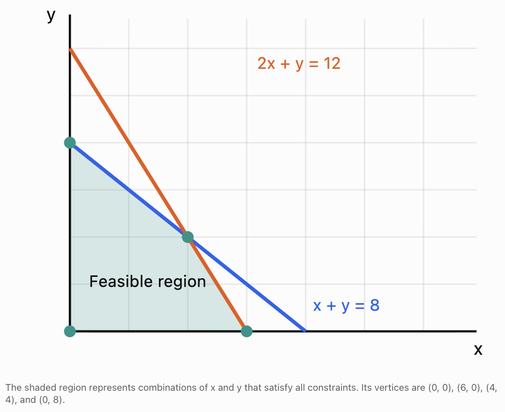
Every point inside or on the boundary of the feasible region is an allowable solution.

Points outside the region violate at least one constraint.

Linear Programming

Linear programming is the process of optimising a linear objective function subject to linear constraints.

When there are two decision variables, many problems can be solved graphically.

An important result is that if a linear objective has a maximum or minimum over a nonempty, bounded polygonal feasible region, at least one optimal solution occurs at a vertex.

This is called the corner-point principle.

Worked Example 2: Maximising Factory Profit

A factory manufactures two products.

Product A earns $40 profit per unit.

Product B earns $30 profit per unit.

The constraints are:

Find the maximum possible profit.

Step 1: Write the objective function

Step 2: Find the vertices of the feasible region

The vertices include:

(0, 0)

(50, 0)

(0, 40)

We must also find the intersection of:

2x + y = 100

x + 2y = 80

From the first equation:

y = 100 − 2x

Substitute into the second:

x + 2(100 − 2x) = 80

x + 200 − 4x = 80

−3x = −120

Then:

The intersection is:

(40, 20)

Step 3: Evaluate the objective at each vertex

Step 4: Identify the maximum

The greatest profit is $2,200.

Therefore:

The factory should produce 40 units of A and 20 units of B.

Step 5: Interpret the result

Both resource constraints are fully used:

This means the optimal solution uses all available quantities of both constrained resources.

Integer Programming

Some optimisation variables must be whole numbers.

For example:

• Number of vehicles.

• Number of employees.

• Number of machines.

• Number of products.

• Number of classrooms.

A solution such as 3.7 vehicles is not meaningful.

An integer programming problem includes restrictions requiring selected variables to be integers.

Worked Example 3: Whole-Number Production

A workshop produces chairs and tables.

Let:

x = number of chairs.

y = number of tables.

The profit is:

The constraints are:

and x and y must be integers.

The intersection of the two boundary lines is:

x + 2y = 9

2x + y = 10

Multiply the first equation by 2:

2x + 4y = 18

Subtract the second:

3y = 8

Then:

The continuous intersection is:

But fractional chairs and tables are not allowed.

We must examine feasible integer combinations.

The highest profit among these feasible combinations is $195. To verify global optimality, note that for each integer y = 0, 1, 2, 3, 4, the maximum feasible x is respectively 5, 4, 4, 3, 1. Their best profits are $125, $140, $180, $195, and $185.

Therefore:

This illustrates why integer constraints can change an optimisation problem.

Optimisation with Several Variables

Many real problems involve more than two variables.

Suppose a delivery company uses three types of vehicles.

Let:

x₁ = number of small vehicles.

x₂ = number of medium vehicles.

x₃ = number of large vehicles.

Suppose operating costs are:

$80, $120, and $180 per vehicle.

The cost function is:

In vector form:

where:

The company may need to satisfy capacity requirements:

and a vehicle availability constraint:

The objective is to minimise cost.

This model is an integer linear programming problem if all vehicle counts must be whole numbers.

In higher-dimensional problems, graphical methods become impractical.

Algorithms such as the simplex method, interior-point methods, and branch-and-bound are used to solve appropriate optimisation problems.

Quadratic Optimisation

Not all optimisation problems have linear objective functions.

A quadratic objective function contains squared variables or products of variables.

For example:

This function measures the squared distance of a point (x, y) from the origin.

To minimise it without additional constraints:

Therefore:

Matrix Form of a Quadratic Function

A quadratic function can be written using matrices:

where Q is a square matrix.

For example:

and:

Then:

Quadratic optimisation is used in:

• Engineering design.

• Portfolio optimisation.

• Control systems.

• Statistical modelling.

• Machine learning.

Optimisation Using Calculus

Calculus provides methods for finding maximum and minimum values of differentiable functions.

For a function of one variable:

stationary points occur where:

These points may be maxima, minima, or neither.

Worked Example 4: Minimising a Cost Function

Suppose the cost of operating a machine is modelled by:

where x represents an adjustable operating setting.

Find the value of x that minimises cost.

Step 1: Differentiate

Step 2: Set the derivative equal to zero

Step 3: Confirm a minimum

Since:

the function has a minimum at x = 10.

Step 4: Calculate the minimum cost

The minimum cost is 100 cost units at operating setting x = 10.

Optimisation with Multiple Variables

For a function involving several variables:

we use partial derivatives.

The gradient is:

At an interior stationary point of a differentiable function:

Worked Example 5: Minimising a Two-Variable Function

Find the minimum of:

Step 1: Calculate partial derivatives

Step 2: Set both equal to zero

Step 3: Evaluate the function

Step 4: Confirm the minimum

Complete the square:

Since squared terms cannot be negative:

at:

This is the global minimum.

The Hessian Matrix

For functions involving multiple variables, second derivatives can be organised into a matrix called the Hessian.

For f(x, y):

For:

the Hessian is:

This matrix is positive definite.

Therefore, the stationary point is a strict local minimum.

Because the function is a convex quadratic, it is also the global minimum.

Interpreting the Hessian

At a stationary point:

• A positive definite Hessian indicates a strict local minimum.

• A negative definite Hessian indicates a strict local maximum.

• An indefinite Hessian indicates a saddle point.

• A semidefinite Hessian may require further analysis.

The Hessian connects multivariable calculus directly to matrix algebra.

Least-Squares Optimisation

A major application of optimisation is finding a mathematical model that fits observed data.

Suppose a linear model is:

We want to choose m and b so that predictions are close to the actual observations.

The least-squares objective is:

The goal is to minimise SSE.

Matrix Representation

A linear model can be written as:

where:

• A is the design matrix.

• β is the vector of model parameters.

• y is the vector of observed values.

The least-squares problem is:

When A has linearly independent columns, the unique least-squares solution satisfies:

These are called the normal equations.

If AᵀA is invertible:

In practical numerical computing, QR factorisation or singular value decomposition is often preferred to explicitly forming this inverse.

Worked Example 6: Fitting a Line

Suppose the observations are:

Find the least-squares regression line.

We use:

The means are:

The slope is:

Numerator:

Denominator:

Therefore:

The intercept is:

The regression equation is:

This line minimises the sum of squared vertical residuals for the observations.

Gradient Descent

Some optimisation problems are too large or complicated to solve directly.

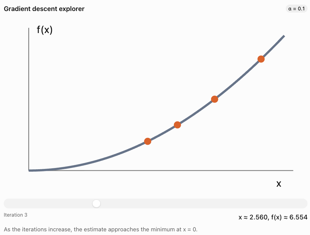
Gradient descent is an iterative method that adjusts variables in the direction opposite to the gradient.

The update rule is:

where:

• xₖ is the current estimate.

• α is the learning rate or step size.

• ∇f is the gradient.

The gradient points in the direction of steepest local increase, so moving against it can reduce the objective function.

Worked Example 7: Gradient Descent

Consider:

The derivative is:

Start with:

x₀ = 5

Use learning rate:

α = 0.1

The update rule is:

First iteration:

Second iteration:

Third iteration:

The values move toward zero, where f(x) reaches its minimum.

Choosing a Learning Rate

If the learning rate is too small, convergence may be slow.

If it is too large, the algorithm may overshoot the minimum or fail to converge.

Gradient descent is widely used in machine learning, optimisation, and scientific computing.

Constrained Optimisation Using Lagrange Multipliers

Some optimisation problems involve equality constraints.

For example, we may want to maximise a function:

subject to:

The method of Lagrange multipliers introduces a new variable λ.

At a suitable constrained optimum:

together with:

Worked Example 8: Maximum Product with Fixed Sum

Find the maximum value of:

subject to:

with x, y ≥ 0.

The gradients are:

Set:

Therefore:

y = λ

x = λ

Hence:

x = y

Using the constraint:

x + y = 10

2x = 10

x = 5

y = 5

Therefore:

We can verify this result using substitution:

This is a downward-opening parabola with maximum at x = 5.

The maximum product occurs when the two nonnegative numbers are equal.

Mathematical Modelling in Engineering

Engineering optimisation often involves balancing competing requirements.

For example, a structural engineer may want to minimise the mass of a component while ensuring that it can support a specified load.

A general engineering optimisation model might be:

subject to:

and:

where the decision vector x may contain dimensions, material quantities, or operating parameters.

The constraints may represent:

• Maximum stress.

• Minimum strength.

• Maximum displacement.

• Available materials.

• Safety requirements.

• Manufacturing limitations.

Example: Minimising Material Cost

Suppose a rectangular container has a fixed volume:

The surface area of a closed rectangular container is:

If material cost is proportional to surface area, minimising material cost means minimising S.

The constraint is:

This is a nonlinear constrained optimisation problem.

For a closed rectangular box with a fixed positive volume and no other restrictions, the minimum surface area occurs when:

The optimal shape is a cube.

This result illustrates how mathematical modelling can guide engineering design.

Optimisation in Transportation and Logistics

Transport companies frequently solve optimisation problems involving:

• Vehicle capacity.

• Delivery demand.

• Fuel consumption.

• Travel time.

• Driver availability.

• Storage limitations.

Worked Example 9: A Transportation Model

A supplier has two warehouses and two stores.

Warehouse A can supply 40 units.

Warehouse B can supply 60 units.

Store 1 requires 50 units.

Store 2 requires 50 units.

Shipping costs per unit are:

Let:

x₁₁ = units shipped from A to Store 1.

x₁₂ = units shipped from A to Store 2.

x₂₁ = units shipped from B to Store 1.

x₂₂ = units shipped from B to Store 2.

The objective is:

Constraints:

Warehouse A:

Warehouse B:

Store 1:

Store 2:

All variables must be nonnegative.

Step 1: Express all variables using one variable

Let:

Then:

Non-negativity requires:

Step 2: Substitute into the cost function

Expand:

Simplify:

Step 3: Minimise cost

Since the coefficient of t is negative, cost decreases as t increases.

Therefore, choose the largest feasible value:

Step 4: Calculate shipment quantities

Step 5: Calculate minimum cost

The optimal shipping plan is:

• 40 units from Warehouse A to Store 1.

• 10 units from Warehouse B to Store 1.

• 50 units from Warehouse B to Store 2.

Multi-Objective Optimisation

Some problems have more than one objective.

For example, a company may want to:

• Minimise cost.

• Maximise quality.

• Minimise environmental impact.

• Maximise customer satisfaction.

These objectives may conflict.

A cheaper solution may produce lower quality.

A more environmentally sustainable solution may have higher initial costs.

Weighted Objective Functions

One approach combines objectives using weights.

Suppose:

C = cost.

E = environmental impact.

We may minimise:

where α and β represent the relative importance of each objective.

The quantities should be scaled appropriately before combining them, especially when measured in different units.

Pareto Optimality

A solution is Pareto optimal if no objective can be improved without making at least one other objective worse.

Rather than producing a single best solution, multi-objective optimisation may produce a collection of reasonable trade-offs.

This collection is called the Pareto frontier.

Evaluating Mathematical Models

A mathematically correct solution is not necessarily a useful real-world solution.

A model must also be evaluated in terms of its assumptions, limitations, and practical meaning.

Important Questions

1. Are the assumptions reasonable?

For example, does the model assume constant costs when costs actually change with production volume?

2. Are the variables clearly defined?

Every variable should have a precise interpretation and appropriate units.

3. Are all important constraints included?

A production model may be unrealistic if it ignores storage, labour availability, or maintenance.

4. Is the objective appropriate?

Maximising short-term profit may not be the same as maximising long-term sustainability.

5. Are the data reliable?

Incorrect estimates of cost, demand, or capacity may lead to poor decisions.

6. Is the solution practical?

A mathematically optimal solution may require fractional machines, impossible schedules, or unavailable resources.

7. How sensitive is the solution?

Would a small change in input data produce a very different answer?

Sensitivity Analysis

Sensitivity analysis examines how changes in model parameters affect the optimal solution.

Suppose a company maximises:

If the profit per unit of Product B increases from $30 to $50, the objective becomes:

The best production combination may change.

Worked Example 10: Sensitivity of an Optimal Solution

Return to the feasible vertices from Worked Example 2:

(0, 0), (50, 0), (0, 40), and (40, 20).

The new profit function is:

Evaluate:

Therefore:

The optimal production quantities remain:

Although the profit increased, the optimal production combination did not change.

This demonstrates that some optimisation solutions are stable under certain changes in model parameters.

Choosing an Appropriate Optimisation Method

Different problems require different mathematical techniques.

The best method depends on the mathematical structure of the problem.

Real-World Applications

Common Mistakes

Mistake 1: Confusing decision variables with fixed parameters

Decision variables are quantities we choose. Parameters are values supplied by the model.

Mistake 2: Writing an objective function without defining the variables

Every variable must have a clear interpretation.

Mistake 3: Forgetting constraints

An unconstrained maximum may be unrealistic or unbounded.

Mistake 4: Using the wrong inequality direction

For example, a maximum resource limit requires ≤, while a minimum demand requirement often requires ≥.

Mistake 5: Forgetting non-negativity restrictions

Negative production quantities or vehicle counts are usually not meaningful.

Mistake 6: Assuming every feasible solution is optimal

A feasible solution satisfies the constraints, but it may not maximise or minimise the objective.

Mistake 7: Assuming the optimum always occurs at a corner

The corner-point principle applies to linear objectives over appropriate polyhedral feasible regions. Nonlinear objectives may have interior optima.

Mistake 8: Ignoring integer restrictions

A fractional solution may not be practical when variables represent indivisible objects.

Mistake 9: Confusing local and global optima

A local optimum is best within a nearby region. A global optimum is best over the entire feasible set.

Mistake 10: Assuming every stationary point is a minimum

Stationary points may be minima, maxima, or saddle points.

Mistake 11: Applying matrix formulas without checking dimensions

Matrix multiplication requires compatible dimensions.

Mistake 12: Assuming the inverse of AᵀA always exists

The inverse requires the columns of A to be linearly independent.

Mistake 13: Choosing a learning rate without considering convergence

An inappropriate step size can slow or destabilise gradient descent.

Mistake 14: Ignoring model assumptions

A mathematically valid answer may not represent real conditions accurately.

Mistake 15: Treating an optimal solution as permanently optimal

Changes in prices, demand, resource availability, or constraints may change the best solution.

Key Terms

• Optimisation: Process of finding the best value of an objective under specified conditions.

• Mathematical Model: Mathematical representation of a real-world system.

• Decision Variable: Quantity selected or controlled in an optimisation problem.

• Parameter: Fixed numerical value used in a model.

• Objective Function: Function to be maximised or minimised.

• Constraint: Restriction on allowable solutions.

• Feasible Solution: Solution satisfying every constraint.

• Feasible Region: Set of all feasible solutions.

• Optimal Solution: Feasible solution producing the best objective value.

• Linear Programming: Optimisation involving linear objectives and constraints.

• Integer Programming: Optimisation requiring some or all decision variables to be integers.

• Corner-Point Principle: Property that a bounded linear programming problem with an optimum has an optimal vertex solution.

• Dot Product: Scalar obtained by multiplying and summing corresponding vector components.

• Constraint Matrix: Matrix containing coefficients of linear constraints.

• Quadratic Optimisation: Optimisation involving quadratic objective functions.

• Gradient: Vector of first-order partial derivatives.

• Stationary Point: Point where the gradient is zero, when the gradient exists.

• Hessian Matrix: Matrix of second-order partial derivatives.

• Positive Definite Matrix: Symmetric matrix for which xᵀAx is positive for every nonzero vector x.

• Convex Function: Function whose graph lies below or on the line segment connecting any two points on its graph.

• Local Minimum: Minimum within a neighbourhood of a point.

• Global Minimum: Smallest function value over the entire feasible domain.

• Least Squares: Method minimising the sum of squared residuals.

• Residual: Difference between an observed value and a predicted value.

• Design Matrix: Matrix representing predictor variables in a statistical model.

• Gradient Descent: Iterative optimisation method using the negative gradient.

• Learning Rate: Step size used in gradient-based optimisation.

• Lagrange Multiplier: Auxiliary variable used to analyse constrained optima.

• Sensitivity Analysis: Study of how changes in parameters affect model results.

• Multi-Objective Optimisation: Optimisation involving several objectives.

• Pareto Optimality: Condition where improving one objective necessarily worsens another.

• Pareto Frontier: Set of non-dominated trade-off solutions.

• Model Validation: Process of checking whether a model adequately represents the intended system.

Key Takeaways

• Optimisation involves maximising or minimising an objective while satisfying constraints.

• Decision variables can be organised into vectors.

• Linear objective functions can be expressed using dot products.

• Systems of linear constraints can be represented using matrices.

• The feasible region contains every solution satisfying all constraints.

• Linear programming optimises linear objectives subject to linear constraints.

• For suitable two-variable linear programming problems, optimal solutions can be found by evaluating vertices.

• Integer programming is necessary when some variables must represent whole-number quantities.

• Quadratic optimisation involves squared variables and can be represented using matrix expressions.

• Differentiation and partial derivatives help identify stationary points.

• The Hessian matrix helps classify stationary points of multivariable functions.

• Least-squares optimisation is used to fit mathematical models to observed data.

• Gradient descent provides an iterative method for minimising differentiable objective functions.

• Lagrange multipliers help solve equality-constrained optimisation problems.

• Transportation and production problems can be modelled using matrices and linear constraints.

• Multi-objective optimisation considers trade-offs between competing goals.

• Sensitivity analysis reveals how model results respond to changing assumptions.

• A mathematically optimal solution must still be evaluated for realism, feasibility, and usefulness.

Check Your Understanding

Questions

Question 1: Objective Functions

A company produces two products.

Product A earns $15 profit per unit.

Product B earns $25 profit per unit.

Write an objective function for total profit.

Question 2: Vector Representation

A manufacturer produces three products with profits of $10, $20, and $30 per unit.

Write the profit coefficient vector.

Question 3: Dot Product

Given:

and:

Calculate cᵀx.

Question 4: Matrix Constraints

Write the following system in matrix form:

Question 5: Feasibility

Determine whether the point (5, 10) satisfies:

Question 6: Linear Programming

Maximise:

subject to:

Find the maximum value of P.

Question 7: Integer Programming

Explain why a company purchasing delivery trucks may require an integer programming model.

Question 8: Quadratic Optimisation

Find the minimum value of:

Question 9: Multivariable Optimisation

Find the minimum of:

Question 10: Gradient Descent

For:

start at x = 4 with learning rate α = 0.25.

Calculate the next two iterations.

Question 11: Least Squares

Actual values are:

10, 15, 20

Predicted values are:

12, 14, 19

Calculate the sum of squared errors.

Question 12: Transportation Costs

A company ships:

• 20 units at $4 per unit.

• 30 units at $6 per unit.

• 10 units at $8 per unit.

Calculate total shipping cost using a dot product.

Question 13: Sensitivity Analysis

A product earns $20 profit per unit.

The company produces 50 units.

Calculate total profit.

Then calculate the new profit if profit per unit increases to $24.

Question 14: Model Evaluation

Explain three reasons why a mathematically optimal solution might not be suitable in practice.

Question 15: Integrated Optimisation Challenge

A company produces two products, A and B.

Profit per unit:

A: $50

B: $40

Production constraints:

a) Define the decision variables.

b) Write the objective function.

c) Express the constraints in matrix form.

d) Find the vertices of the feasible region.

e) Calculate profit at each vertex.

f) Determine the optimal production quantities.

g) Calculate maximum profit.

h) Explain two assumptions of the model.

i) Explain how the model could be improved.

Fully Worked Answers

Answer 1: Objective Functions

Let:

x = number of units of A.

y = number of units of B.

Profit from A:

15x

Profit from B:

25y

Therefore:

The objective is to maximise P.

Answer 2: Vector Representation

The profit coefficient vector is:

Answer 3: Dot Product

Answer 4: Matrix Constraints

The system is:

Therefore:

Answer 5: Feasibility

Substitute:

x = 5

y = 10

First constraint:

Since:

20 ≤ 25

the first constraint is satisfied.

Second constraint:

Since:

35 ≤ 40

the second constraint is satisfied.

Therefore:

Answer 6: Linear Programming

Objective:

Constraints:

The vertices are:

(0, 0)

(6, 0)

(6, 4)

(2, 8)

(0, 8)

Evaluate:

Therefore:

at:

Answer 7: Integer Programming

Delivery trucks cannot normally be purchased in fractional quantities.

A mathematical solution such as 4.6 trucks is not physically meaningful.

Therefore, the number of trucks must be restricted to nonnegative integers.

An integer programming model includes these restrictions.

Answer 8: Quadratic Optimisation

Given:

Differentiate:

Set equal to zero:

Evaluate:

Since the coefficient of x² is positive, the parabola opens upward and this is the global minimum.

Answer 9: Multivariable Optimisation

Given:

Partial derivatives:

Set equal to zero:

Evaluate:

Complete the square:

Therefore:

at:

Answer 10: Gradient Descent

Given:

Derivative:

Update rule:

Start:

x₀ = 4

First iteration:

Second iteration:

Therefore:

Answer 11: Least Squares

Residuals:

10 − 12 = −2

15 − 14 = 1

20 − 19 = 1

Square:

4, 1, 1

Add:

Answer 12: Transportation Costs

Cost vector:

Quantity vector:

Total cost:

Answer 13: Sensitivity Analysis

Original profit:

New profit:

Increase:

The total profit increases by $200, assuming the production quantity remains unchanged.

Answer 14: Model Evaluation

Three possible reasons are:

Unrealistic assumptions: The model may assume constant costs or unlimited demand when these conditions do not hold.

Missing constraints: The model may ignore labour availability, safety requirements, storage capacity, or environmental regulations.

Practical limitations: The solution may require fractional quantities, unavailable equipment, or unrealistic operating schedules.

A useful optimisation model must represent the important features of the real system.

Answer 15: Integrated Optimisation Challenge

Part a: Define variables

Let:

x = number of units of Product A.

y = number of units of Product B.

Part b: Objective function

The objective is to maximise P.

Part c: Matrix constraints

with:

Part d: Find the vertices

On the x-axis:

2x ≤ 100

Therefore:

x ≤ 50

Vertex:

(50, 0)

On the y-axis:

2y ≤ 80

Therefore:

y ≤ 40

Vertex:

(0, 40)

The origin is:

(0, 0)

Now solve:

2x + y = 100

x + 2y = 80

From the first equation:

y = 100 − 2x

Substitute:

x + 2(100 − 2x) = 80

x + 200 − 4x = 80

−3x = −120

Then:

Intersection:

(40, 20)

Therefore, the vertices are:

(0, 0), (50, 0), (0, 40), (40, 20).

Part e: Evaluate profit

Part f: Optimal production

Part g: Maximum profit

Part h: Two assumptions

The model assumes that profit per unit remains constant regardless of production quantity.

It also assumes that the two resource constraints represent the important limitations on production.

Part i: Improvements

The model could be improved by including additional constraints such as labour availability, storage, customer demand, and machine maintenance.

It could also include changing production costs, uncertain demand, and sensitivity analysis.

These improvements would make the model more realistic and useful for decision-making.

Final Reflection

Optimisation and mathematical modelling connect abstract mathematical ideas with practical decision-making.

Vectors provide an organised way to represent decision variables. Matrices allow many constraints to be written and analysed efficiently. Linear programming identifies optimal solutions under linear restrictions, while calculus and quadratic optimisation extend these ideas to nonlinear relationships.

Least-squares methods and gradient descent demonstrate how optimisation is used to construct mathematical models from data. Engineering, transportation, economics, and artificial intelligence all rely on these techniques.

However, finding a mathematical optimum is only one part of solving a real-world problem. A successful model must also use realistic assumptions, appropriate constraints, reliable data, and meaningful interpretations.

The central idea is that optimisation uses mathematical models to identify the best available decisions while respecting the limitations and requirements of real systems.