Advanced Applications and Mathematical Connections

Introduction

Every day, enormous amounts of data are generated through smartphones, websites, scientific instruments, medical equipment, financial systems, and digital devices.

Data science is the study of how information can be collected, organised, analysed, and used to identify patterns or make predictions.

Artificial intelligence (AI) uses computational systems to perform tasks such as recognising images, understanding language, identifying patterns, and making decisions or predictions.

Although these technologies can appear extremely complicated, many of their mathematical foundations come from two familiar ideas:

Vectors and matrices.

A photograph can be represented by numbers arranged in matrices. A person's preferences can be represented by a vector. A collection of measurements can be organised into a data matrix. A neural network can transform information using repeated matrix multiplication.

Linear algebra provides the mathematical language that connects these applications.

In this lesson, we will explore how vectors represent data, how matrices organise information, how machine learning systems use matrix operations, and why vector spaces are essential to modern artificial intelligence.

Representing Data Using Vectors

A data vector is an ordered collection of numerical values representing the features of an object, observation, or event.

A feature is a measurable characteristic.

For example, a student might be described using:

• Hours studied per week.

• Number of assignments completed.

• Average assessment score.

Suppose a student studies 8 hours per week, completes 12 assignments, and has an average score of 85%.

We can represent this information as:

Each component represents a different feature.

The vector contains three components, so it belongs to the three-dimensional vector space ℝ³.

However, these dimensions do not necessarily represent physical directions.

Instead, each dimension represents a different characteristic of the data.

Why Represent Data as Vectors?

Vectors allow computers to perform mathematical operations on information.

For example, they can be used to:

• Compare observations.

• Measure similarities.

• Identify patterns.

• Calculate predictions.

• Group related objects.

• Transform data.

• Train machine learning models.

Worked Example 1: Constructing a Data Vector

A car has the following characteristics:

Represent the car as a feature vector.

The vector is:

This vector belongs to ℝ⁴.

It contains four numerical features describing the car.

Important: The order of features must remain consistent when comparing different cars. The numerical components also have different units and scales, which may need to be adjusted before analysis.

Data Matrices

A data matrix is a rectangular arrangement of numerical data.

In many datasets:

• Each row represents an observation.

• Each column represents a feature.

Suppose we collect information from four students.

The data matrix is:

This is a 4 × 3 matrix.

It contains:

• 4 observations.

• 3 features.

The matrix belongs to ℝ⁴ˣ³, the space of real 4 × 3 matrices.

Why Matrices Are Useful

Instead of processing every observation separately, a computer can process many observations simultaneously using matrix operations.

This makes matrices particularly useful for large datasets containing thousands or millions of observations.

Matrix Operations in Data Science

Several familiar matrix operations appear repeatedly in data science.

Matrix Addition

Matrices of the same dimensions can be added element by element.

Suppose two sensors record measurements:

Then:

Matrix addition can combine compatible numerical datasets or model contributions from different sources.

Scalar Multiplication

A matrix can be multiplied by a scalar.

For example:

Multiplying by 0.5 gives:

Scalar multiplication is useful when rescaling numerical information.

Matrix Multiplication

Matrix multiplication combines information according to mathematical relationships between rows and columns.

If A is an m × n matrix and B is an n × p matrix, then:

The inner dimensions must match.

Matrix multiplication is one of the most important operations in machine learning.

Weighted Predictions Using Vectors

Many machine learning models calculate predictions using weighted combinations of input features.

A weight describes how strongly a feature contributes to a prediction.

Suppose a simple model estimates a student's performance using:

• Study hours.

• Assignments completed.

The feature vector is:

The weight vector is:

The prediction is calculated using the dot product:

where:

• ŷ is the predicted value.

• w is the weight vector.

• x is the feature vector.

• b is a bias or intercept.

Worked Example 2: Making a Prediction

Suppose:

and:

b = 15

Calculate the prediction.

The model predicts a score of 77.

This is an illustrative mathematical model. In a real machine learning application, the weights and bias would normally be estimated from training data.

Matrix Multiplication for Multiple Predictions

Suppose we want to make predictions for three students.

Their features are:

The weights are:

We calculate:

Multiply each row by the weight vector.

First student:

4(4) + 6(3) = 34

Second student:

6(4) + 8(3) = 48

Third student:

8(4) + 10(3) = 62

Therefore:

If the bias is 15, add 15 to every prediction:

A single matrix multiplication produces predictions for multiple observations.

This approach is fundamental to efficient machine learning.

Linear Regression and Matrix Models

Linear regression is a method for modelling relationships between numerical variables.

For one input feature:

For several input features:

In matrix form, predictions for many observations can be written as:

where 1 is a column vector of ones.

The model uses the features and weights to generate predictions.

Training a Regression Model

The goal is to find weights that produce predictions close to the observed values.

The difference between an observed value and a predicted value is called a residual.

One common training method minimises the sum of squared residuals:

This is called the least-squares method.

Worked Example 3: Calculating Prediction Errors

A model predicts:

Calculate the sum of squared errors.

Residuals:

Observation 1:

60 − 58 = 2

Observation 2:

70 − 73 = −3

Observation 3:

80 − 78 = 2

Square the residuals:

2² = 4

(−3)² = 9

2² = 4

Add:

A smaller SSE generally indicates a closer fit to the training observations, although model complexity and performance on new data must also be considered.

Feature Scaling and Normalisation

Real datasets often contain features measured on very different scales.

For example:

If these values are used directly, some methods may be strongly influenced by features with larger numerical scales.

Feature scaling transforms numerical values so that different features can be compared more appropriately.

Min-Max Scaling

One method is:

This transforms values into the interval from 0 to 1 when the minimum and maximum are distinct.

Worked Example 4: Scaling Data

Suppose test scores range from 40 to 100.

A student scores 70.

Calculate the scaled score.

The scaled score is 0.5.

Standardisation

Another common method is:

where:

• μ is the mean.

• σ is the standard deviation.

Standardisation produces values measured in standard deviations from the mean.

It is especially useful in many statistical and machine learning methods.

Important: Scaling parameters should normally be calculated using the training dataset and then applied consistently to validation and test data to avoid information leakage.

Measuring Similarity Between Data Vectors

One of the most important tasks in artificial intelligence is determining how similar two objects are.

Objects may be represented as vectors containing numerical features.

For example, two songs might be described using:

• Tempo.

• Energy.

• Danceability.

• Instrumental characteristics.

Two images might be represented using features describing shapes, colours, and textures.

Two documents might be represented using numerical information about their meaning or word usage.

Euclidean Distance

The Euclidean distance between two vectors is:

In two dimensions:

Smaller distances indicate that vectors are closer together.

Worked Example 5: Comparing Two Data Vectors

Suppose:

Calculate their Euclidean distance.

The two vectors are 5 units apart.

Cosine Similarity

Euclidean distance measures how far apart vectors are.

Cosine similarity measures how closely their directions align.

For nonzero vectors:

Cosine similarity ranges from −1 to 1.

• 1 means the vectors point in the same direction.

• 0 means the vectors are perpendicular.

• −1 means the vectors point in opposite directions.

For many applications involving nonnegative feature vectors, cosine similarity is between 0 and 1.

Worked Example 6: Calculating Cosine Similarity

Given:

Calculate cosine similarity.

Dot product:

Magnitudes:

Therefore:

The vectors point in exactly the same direction.

This does not mean the vectors have the same magnitude.

Cosine similarity is widely used in document retrieval, recommendation systems, and comparisons between numerical representations of language.

Vector Spaces in Artificial Intelligence

Artificial intelligence often represents information in high-dimensional vector spaces.

A vector space with n coordinates is written:

For example:

• A two-feature dataset uses ℝ².

• A dataset with ten numerical features uses ℝ¹⁰.

• A representation containing 512 numerical features uses ℝ⁵¹².

These spaces cannot always be visualised directly, but the same mathematical operations still apply.

Vectors can be added, multiplied by scalars, compared using distances, and transformed using matrices.

Embeddings

An embedding is a numerical vector representation of an object, such as a word, sentence, image, or product.

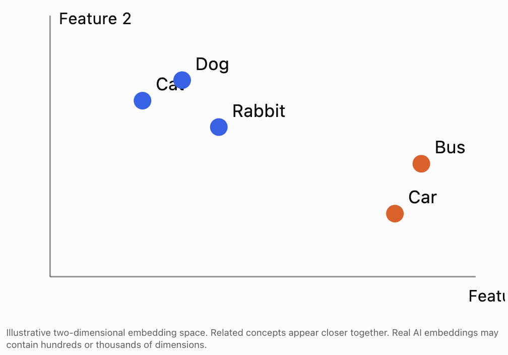
For example, a hypothetical AI system might represent three words using vectors:

These values are illustrative rather than actual embeddings from a trained model.

The vectors for cat and dog are close together, while car is farther away.

In a trained embedding system, such relationships may reflect similarities learned from data.

Why Embeddings Matter

Embeddings make it possible to compare information mathematically.

They are used in:

• Search engines.

• Language models.

• Recommendation systems.

• Image retrieval.

• Document classification.

• Semantic search.

However, the numerical meaning of each individual embedding coordinate is not always directly interpretable.

Matrices in Neural Networks

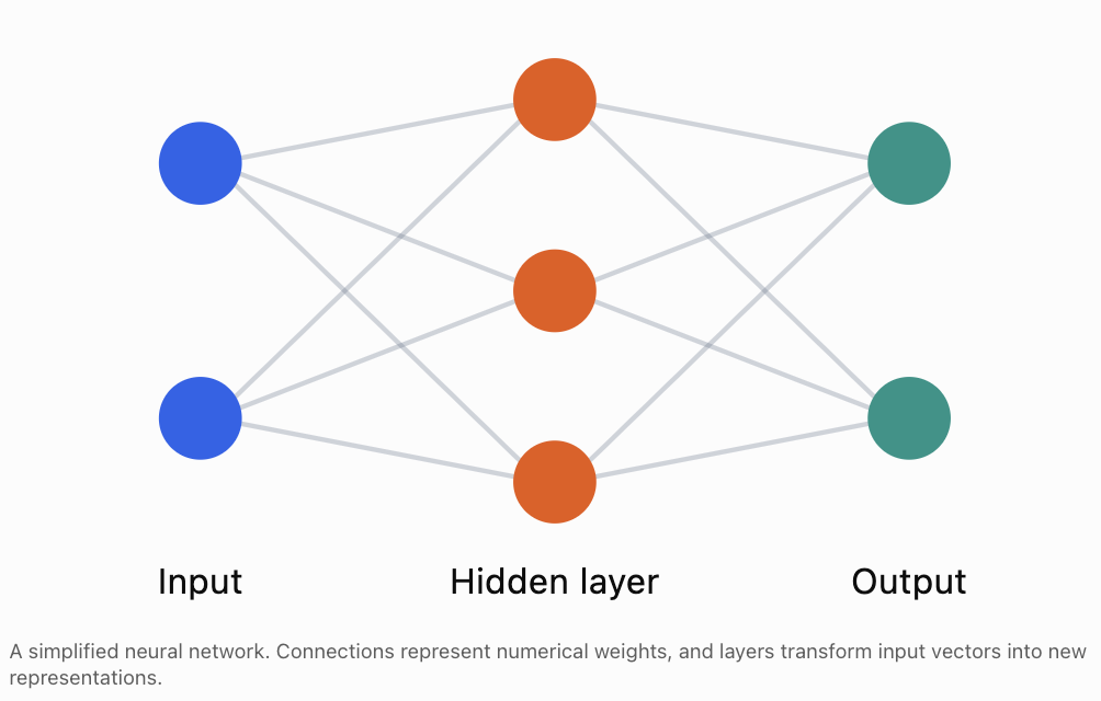
A neural network is a computational model containing layers of interconnected numerical operations.

Many neural networks use matrix multiplication to transform input data.

A basic layer can be written as:

where:

• x is the input vector.

• W is a weight matrix.

• b is a bias vector.

• z is the output before applying an activation function.

An activation function is often applied:

The activation function introduces nonlinearity, allowing neural networks to represent relationships more complex than a single linear transformation.

Worked Example 7: A Simple Neural Network Layer

Suppose:

Input:

Bias:

Calculate:

First multiply:

Add the bias:

If the layer uses the ReLU activation function:

then:

The output is the transformed feature vector.

How Neural Networks Learn

A neural network begins with numerical weights and biases.

During training, the network processes examples and compares its predictions with known targets.

A loss function measures prediction error.

The training process then adjusts the weights and biases to reduce the loss.

A common optimisation method is gradient descent.

For a parameter w:

where:

• L is the loss function.

• α is the learning rate.

• dL/dw is the derivative of loss with respect to the weight.

For many parameters collected into a vector:

The gradient indicates how the loss changes as the parameters change.

Worked Example 8: One Gradient Descent Step

Suppose:

w = 5

Learning rate:

α = 0.1

Gradient:

dL/dw = 6

Calculate the updated weight.

The weight decreases from 5 to 4.4.

This is one small step in the training process.

Modern neural networks may contain millions or billions of parameters, and training involves many such updates.

Image Data as Matrices

Digital images are represented using numerical values.

A grayscale image can be stored as a matrix.

Each matrix entry represents the intensity of a pixel.

For a typical 8-bit grayscale image:

• 0 represents black.

• 255 represents white.

• Values between 0 and 255 represent shades of gray.

Consider:

This represents a 3 × 3 grayscale image.

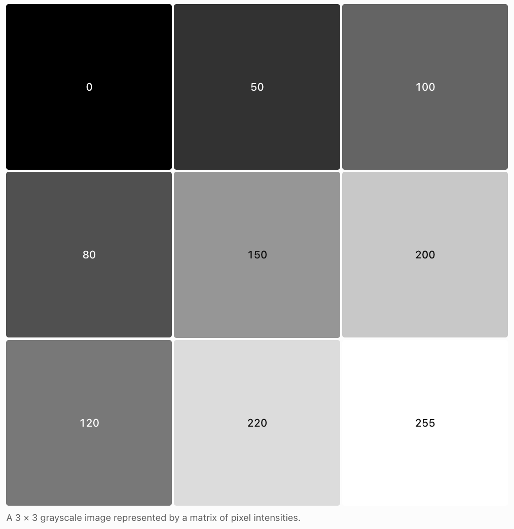
Image Brightness

To increase brightness, a positive value can be added to every pixel.

For example:

Adding 30 gives:

Pixel values must remain within the allowed range.

If a calculation produces a value greater than 255, it may be clipped to 255.

Colour Images

Colour images are commonly represented using three channels:

• Red.

• Green.

• Blue.

Each channel is a matrix.

A colour image can therefore be represented as a three-dimensional array of numerical values.

This representation is used in computer vision and image-processing systems.

Data Transformations and Dimensionality Reduction

Real datasets may contain hundreds or thousands of features.

Some features may be redundant or strongly related.

Dimensionality reduction attempts to represent data using fewer variables while retaining useful information.

One important method is Principal Component Analysis (PCA).

PCA identifies directions in the data along which variation is greatest.

These directions are called principal components.

They are calculated using eigenvectors of a covariance matrix or equivalent numerical methods.

Worked Example 9: A Simple Data Projection

Suppose:

We want to project this vector onto the x-axis.

The projection matrix is:

Calculate:

Therefore:

The original two-dimensional vector has been projected onto a one-dimensional subspace.

This illustrates the basic idea of representing data using fewer dimensions.

PCA chooses projection directions based on the structure of the dataset rather than simply choosing the x-axis.

Recommendation Systems

Recommendation systems suggest products, films, music, or other content based on available information.

One approach represents users and items as vectors in a shared feature space.

For example, a user preference vector might be:

The components might represent preferences for:

• Action.

• Comedy.

• Science fiction.

A film might have feature vector:

A simple compatibility score can be calculated using the dot product.

Worked Example 10: Recommendation Score

A larger dot product may indicate greater compatibility in this simplified model.

However, dot products also depend on vector magnitudes, so real recommendation systems often use normalisation or more sophisticated methods.

Matrices and Modern Computing

Matrix calculations appear throughout modern computing.

Graphics Processing Units

A GPU is a processor designed to perform many calculations in parallel.

GPUs are especially effective for operations involving large arrays and matrices.

This makes them valuable for:

• Computer graphics.

• Scientific simulations.

• Image processing.

• Neural network training.

• Large-scale numerical computing.

Why Matrix Operations Are Efficient

Suppose a neural network needs to process 10,000 observations.

Instead of calculating each prediction separately, the observations can be arranged into a matrix.

The computer can then perform matrix operations on many observations together.

Specialised hardware and numerical libraries can carry out these operations efficiently.

Matrices in Language Models

Language models process text by converting tokens into numerical vector representations.

These vectors are transformed through multiple computational layers.

Matrix multiplication is used extensively in these transformations.

One important mechanism is attention, which helps a model combine information from different positions in a sequence.

A simplified attention calculation is:

where:

• Q contains query vectors.

• K contains key vectors.

• V contains value vectors.

• dₖ is the dimension of each key vector.

• softmax converts numerical scores into relative weights.

This is an advanced example of how linear algebra supports modern AI.

The essential idea is that matrices allow a model to compare and combine many vector representations efficiently.

Real-World Applications

Limitations and Responsible Use of AI

Although vectors and matrices provide powerful tools for analysing data, mathematical models are not automatically accurate or fair.

Several important limitations must be considered.

Data Quality

A model trained using incomplete or inaccurate data may produce unreliable predictions.

Bias

If training data reflects unfair patterns or underrepresents certain groups, a model may reproduce or amplify those patterns.

Overfitting

A model may perform extremely well on training data but poorly on new observations.

This is called overfitting.

Interpretability

Some models are difficult to interpret because their predictions depend on many interacting numerical parameters.

Correlation and Causation

A model may identify statistical relationships without establishing causal explanations.

Privacy

Datasets may contain sensitive information. Responsible systems require appropriate privacy and security safeguards.

Model Evaluation

AI systems should be tested using suitable data and performance measures.

A model's usefulness depends not only on mathematical calculations but also on the quality of its assumptions, data, evaluation, and application.

Common Mistakes

Mistake 1: Assuming every vector represents a physical direction

In data science, vector components often represent features rather than spatial coordinates.

Mistake 2: Mixing up rows and columns in a data matrix

Rows commonly represent observations, while columns represent features, although other conventions are possible.

Mistake 3: Multiplying matrices with incompatible dimensions

The number of columns in the first matrix must equal the number of rows in the second.

Mistake 4: Assuming matrix multiplication is commutative

In general:

AB ≠ BA

Mistake 5: Ignoring feature scales

Features with large numerical values may dominate some calculations unless appropriate scaling is used.

Mistake 6: Confusing Euclidean distance with cosine similarity

Euclidean distance measures separation. Cosine similarity measures directional alignment.

Mistake 7: Assuming a larger dot product always means greater similarity

Dot products depend on both magnitude and direction.

Mistake 8: Thinking neural networks use only linear operations

Nonlinear activation functions are essential for representing many complex relationships.

Mistake 9: Assuming AI models automatically understand the meaning of numbers

The meaning of numerical features depends on how the data is represented and how the model is trained.

Mistake 10: Confusing training accuracy with generalisation

A model may fit training data well but perform poorly on unseen examples.

Mistake 11: Assuming PCA always preserves all information

Dimensionality reduction may discard some information.

Mistake 12: Assuming mathematical predictions are always correct

Predictions depend on the model, its assumptions, and the quality of the data.

Key Terms

• Data Science: Study of collecting, organising, analysing, and interpreting data.

• Artificial Intelligence: Field concerned with computational systems performing tasks associated with intelligent behaviour.

• Machine Learning: Approach in which computational models learn patterns from data.

• Feature: Measurable characteristic used to describe an observation.

• Feature Vector: Ordered collection of numerical features.

• Data Matrix: Matrix containing observations and features.

• Weight: Numerical parameter describing the contribution of a feature or connection.

• Bias: Additive parameter in a mathematical model.

• Prediction: Output estimated by a model.

• Linear Regression: Method for modelling numerical relationships using linear equations.

• Residual: Difference between an observed value and a predicted value.

• Loss Function: Function measuring model error.

• Least Squares: Method that minimises the sum of squared residuals.

• Feature Scaling: Transformation of numerical features to more suitable scales.

• Min-Max Scaling: Method transforming values using their minimum and maximum.

• Standardisation: Transformation expressing values relative to a mean and standard deviation.

• Euclidean Distance: Straight-line distance between vectors.

• Dot Product: Scalar obtained by multiplying and summing corresponding vector components.

• Cosine Similarity: Measure of directional similarity between nonzero vectors.

• Vector Space: Mathematical structure supporting vector addition and scalar multiplication.

• Embedding: Numerical vector representation of an object or concept.

• Neural Network: Computational model consisting of interconnected layers of numerical operations.

• Activation Function: Function applied to a neuron's or layer's numerical output.

• ReLU: Activation function defined by f(x) = max(0, x).

• Gradient Descent: Optimisation method that updates parameters using gradients.

• Learning Rate: Parameter controlling the size of optimisation updates.

• Pixel: Smallest individual element of a raster image.

• Principal Component Analysis: Technique for finding directions of greatest variation in data.

• Dimensionality Reduction: Process of representing data using fewer features.

• Recommendation System: System that predicts or suggests items based on available information.

• GPU: Graphics processing unit designed for highly parallel computation.

• Overfitting: When a model learns training-specific patterns that do not generalise well.

• Generalisation: Ability of a model to perform effectively on new data.

• Attention: Mechanism that combines information using learned relevance weights.

Key Takeaways

• Vectors provide numerical representations of observations and features.

• Data matrices organise multiple observations into rows and features into columns.

• Matrix operations allow computers to process large datasets efficiently.

• Weighted predictions can be calculated using dot products.

• Linear regression uses vectors and matrices to model numerical relationships.

• Feature scaling helps make numerical variables more comparable.

• Euclidean distance measures separation between data vectors.

• Cosine similarity measures directional alignment between vectors.

• AI embeddings represent objects and concepts as vectors in high-dimensional spaces.

• Neural networks use matrix multiplication, biases, and activation functions to transform data.

• Gradient descent adjusts model parameters to reduce prediction error.

• Digital images can be represented using matrices of pixel intensities.

• PCA uses linear algebra to reduce the number of dimensions needed to represent data.

• Recommendation systems can compare user and item vectors.

• GPUs accelerate many large-scale matrix operations.

• Modern language models rely heavily on vector representations and matrix calculations.

• Responsible AI requires attention to data quality, fairness, privacy, and model evaluation.

Check Your Understanding

Questions

Question 1: Feature Vectors

A student has the following characteristics:

• Study hours: 6

• Assignments completed: 9

• Test score: 78

Represent the student as a feature vector.

Question 2: Data Matrices

Three students have the following data:

Construct a data matrix.

Question 3: Matrix Dimensions

A dataset contains 200 observations and 5 numerical features.

What are the dimensions of its data matrix if observations are rows?

Question 4: Matrix Multiplication

Calculate:

Question 5: Weighted Prediction

A prediction model is:

Calculate the prediction when:

x₁ = 5

x₂ = 8

Question 6: Multiple Predictions

Given:

and:

Calculate Xw.

Question 7: Prediction Error

Actual values are:

10, 15, 20

Predicted values are:

12, 14, 18

Calculate the sum of squared errors.

Question 8: Feature Scaling

A dataset has a minimum value of 20 and maximum value of 80.

Calculate the min-max scaled value of 50.

Question 9: Euclidean Distance

Calculate the distance between:

and:

Question 10: Cosine Similarity

Calculate the cosine similarity between:

and:

Question 11: Neural Network Layer

Given:

and:

Calculate Wx + b.

Question 12: Gradient Descent

A weight has initial value 8.

The gradient is 5 and the learning rate is 0.2.

Calculate the updated weight.

Question 13: Image Processing

A grayscale image has pixel matrix:

Increase every pixel value by 20, clipping values at 255 if necessary.

Question 14: Data Science Concepts

Explain the difference between:

a) A feature vector and a data matrix.

b) Euclidean distance and cosine similarity.

c) Training performance and generalisation.

Question 15: Integrated AI Modelling Challenge

A simple AI system predicts the suitability of an educational resource using three features:

• Content quality.

• Difficulty match.

• Student interest.

A resource has feature vector:

The model uses:

and bias:

b = 1

a) Calculate the weighted prediction.

b) Explain the meaning of the weights.

c) Calculate the new prediction if student interest increases from 9 to 10.

d) Explain why this model is linear.

e) Identify two limitations of using this model to recommend educational resources.

Fully Worked Answers

Answer 1: Feature Vectors

The three features are:

Study hours = 6

Assignments completed = 9

Test score = 78

Therefore:

The vector belongs to ℝ³.

Answer 2: Data Matrices

Each row represents one student.

The columns represent study hours and test score.

This is a 3 × 2 matrix.

Answer 3: Matrix Dimensions

There are:

200 observations.

5 features.

Therefore:

The matrix contains 200 rows and 5 columns.

Answer 4: Matrix Multiplication

First row:

2(5) + 3(2) = 16

Second row:

4(5) + 1(2) = 22

Therefore:

Answer 5: Weighted Prediction

Substitute:

Answer 6: Multiple Predictions

First row:

2(3) + 3(2) = 12

Second row:

4(3) + 5(2) = 22

Therefore:

Answer 7: Prediction Error

Residuals:

10 − 12 = −2

15 − 14 = 1

20 − 18 = 2

Square:

(−2)² = 4

1² = 1

2² = 4

Therefore:

Answer 8: Feature Scaling

Substitute:

Answer 9: Euclidean Distance

Answer 10: Cosine Similarity

Dot product:

Both vectors have magnitude 1.

Therefore:

The vectors are perpendicular.

Answer 11: Neural Network Layer

First calculate:

First component:

1(2) + 2(4) = 10

Second component:

3(2) + 1(4) = 10

Therefore:

Add the bias:

Answer 12: Gradient Descent

Substitute:

Answer 13: Image Processing

Original:

Add 20:

All values remain within the permitted range of 0 to 255.

Therefore:

Answer 14: Data Science Concepts

Part a: Feature vector versus data matrix

A feature vector represents the numerical characteristics of one observation.

A data matrix represents multiple observations, usually with each row corresponding to one observation and each column to one feature.

Part b: Euclidean distance versus cosine similarity

Euclidean distance measures the straight-line separation between two vectors.

Cosine similarity measures how closely their directions align.

Part c: Training performance versus generalisation

Training performance measures how well a model fits the examples used during training.

Generalisation describes how well the model performs on new, previously unseen observations.

A model may perform well during training but generalise poorly.

Answer 15: Integrated AI Modelling Challenge

Given:

and:

b = 1

Part a: Weighted prediction

Part b: Meaning of weights

The weights describe how strongly each feature contributes to the model's prediction when the other features remain fixed.

The model gives:

• Content quality a weight of 0.4.

• Difficulty match a weight of 0.3.

• Student interest a weight of 0.2.

The relative importance of these weights depends on how the features are scaled.

Part c: Increased student interest

New feature vector:

Calculate:

The prediction increases by 0.2.

Part d: Why the model is linear

The model uses a weighted sum of the features, followed by addition of a constant bias.

More precisely, it is an affine model because of the nonzero bias. Its dependence on the input features is linear apart from that constant offset.

Part e: Limitations

Two limitations are:

1. The model assumes each feature contributes independently and at a constant rate. Real educational suitability may depend on interactions between features.

2. The model does not include other important factors such as learning style, prior knowledge, accessibility, or resource quality beyond the chosen numerical measures.

Therefore, the model provides a simplified estimate rather than a complete assessment of educational suitability.

Final Reflection

Vectors and matrices are essential mathematical tools in modern data science and artificial intelligence.

Vectors allow numerical information to be represented in a consistent mathematical form. Matrices organise large collections of observations and make it possible to process data efficiently.

Machine learning models use weighted combinations of features to generate predictions. Neural networks extend these ideas through repeated matrix operations and nonlinear transformations.

Vector spaces allow AI systems to represent complex information, including words, images, documents, and user preferences, using high-dimensional numerical representations.

Linear algebra also supports image processing, dimensionality reduction, recommendation systems, optimisation, and large-scale computing.

However, the mathematical power of AI must be combined with careful data collection, responsible model design, appropriate evaluation, and an understanding of limitations.

The central idea is that vectors and matrices transform information into mathematical structures that computers can analyse, compare, and use to identify patterns and generate predictions.