Advanced Applications and Mathematical Connections
2. Linear Algebra Foundations
Learning outcomes
- I can explain the role of vectors and matrices in linear algebra.
- I can identify vector spaces conceptually.
- I can recognise linear independence.
- I can interpret basis vectors.
- I can appreciate the foundations of higher mathematics.
Introduction
Linear algebra is one of the most important branches of modern mathematics. It provides the mathematical foundation for studying vectors, matrices, systems of equations, transformations, and relationships between quantities.
Many mathematical ideas that initially appear unrelated are connected through linear algebra.
For example:
-
A system of simultaneous equations can be represented by a matrix.
-
A geometric transformation can be described using matrix multiplication.
-
A collection of vectors can describe an entire space.
-
A small number of basis vectors can represent infinitely many other vectors.
-
Linear independence helps determine whether mathematical information is redundant.
-
Eigenvalues and eigenvectors reveal important properties of transformations and dynamic systems.
Linear algebra is essential in physics, engineering, computer science, economics, statistics, artificial intelligence, and advanced mathematics.
The central idea is that complicated mathematical structures can often be understood by studying combinations of vectors and the transformations that act on them.
What Is Linear Algebra?
Linear algebra is the branch of mathematics concerned with vectors, vector spaces, linear transformations, matrices, and systems of linear equations.
A relationship is linear when it preserves addition and scalar multiplication in the appropriate mathematical setting.
For example, the equation:
2x + 3y = 12
is a linear equation in two variables.
The system:
2x + 3y = 12
4x − y = 5
can be written as:
Or more simply:
where:
-
A is a matrix of coefficients.
-
x is a vector of unknown quantities.
-
b is a vector of known values.
This equation is one of the fundamental structures of linear algebra.
It appears in scientific modelling, engineering, data analysis, optimisation, and computer simulations.
The Role of Vectors in Linear Algebra
A vector is an object that can be added to another vector and multiplied by a scalar.
In elementary mathematics, vectors are commonly represented as arrows with magnitude and direction.
For example:
This vector represents a displacement of:
-
3 units in the positive x-direction.
-
4 units in the positive y-direction.
Its magnitude is:
However, linear algebra uses a broader understanding of vectors.
Vectors can also represent:
-
Lists of measurements.
-
Forces acting on objects.
-
Electrical currents.
-
Coefficients of polynomials.
-
Images represented by pixel values.
-
Data describing populations.
-
Signals and functions.
The important feature is not necessarily the arrow representation, but the mathematical rules governing vector addition and scalar multiplication.
Vector Addition
Given:
Add corresponding components:
Scalar Multiplication
Multiplying a vector by a scalar changes its magnitude and possibly its direction.
For:
Multiplying by 4 gives:
Multiplying by −1 gives:
The negative scalar reverses the direction of the vector.
These two operations form the basis of vector spaces.
Linear Combinations of Vectors
A linear combination is an expression formed by multiplying vectors by scalars and adding the results.
For two vectors:
where a and b are scalars.
For several vectors:
Linear combinations are fundamental because they allow us to construct new vectors from existing ones.
Worked Example 1: Finding a Linear Combination
Given:
Find:
2u − 3v
First calculate:
Then:
Subtract:
Therefore:
Worked Example 2: Expressing a Vector as a Linear Combination
Given:
Express:
as a linear combination of u and v.
We want:
Therefore:
This produces:
a + b = 6
a − b = 2
Add the equations:
2a = 8
a = 4
Substitute:
4 + b = 6
b = 2
Therefore:
This demonstrates how one vector can be constructed from other vectors.
What Is a Vector Space?
A vector space is a collection of objects called vectors that can be added together and multiplied by scalars while satisfying specific mathematical rules.
For this lesson, we will focus on vector spaces over the real numbers.
A vector space must be closed under two operations:
-
Vector addition.
-
Scalar multiplication.
Closure under addition means that adding two vectors from the space produces another vector in the same space.
Closure under scalar multiplication means that multiplying a vector from the space by any real scalar produces another vector in the same space.
A vector space must also satisfy additional rules, including the existence of a zero vector, additive inverses, and the usual associative and distributive properties.
Example 1: Two-Dimensional Space
The set of all ordered pairs of real numbers is written:
A typical vector is:
where x and y are real numbers.
Examples include:
(2, 3)
(−1, 5)
(0, 0)
(π, √2)
All such vectors belong to ℝ².
If two vectors in ℝ² are added, the result remains in ℝ².
If a vector in ℝ² is multiplied by a real number, the result remains in ℝ².
Therefore, ℝ² is a vector space.
Example 2: Three-Dimensional Space
The set:
contains all ordered triples of real numbers.
A typical vector is:
This space is used extensively in physics, engineering, and computer graphics.
Example 3: Polynomial Vector Spaces
Consider all polynomials of degree at most 2:
where a, b, and c are real numbers.
Two such polynomials can be added:
The result is another polynomial of degree at most 2.
Multiplying by a scalar also produces a polynomial of degree at most 2.
Therefore, these polynomials form a vector space.
Notice that the objects are functions rather than arrows.
This is an important example of the abstract nature of linear algebra.
Vector Spaces and Subspaces
A subspace is a smaller vector space contained within a larger vector space.
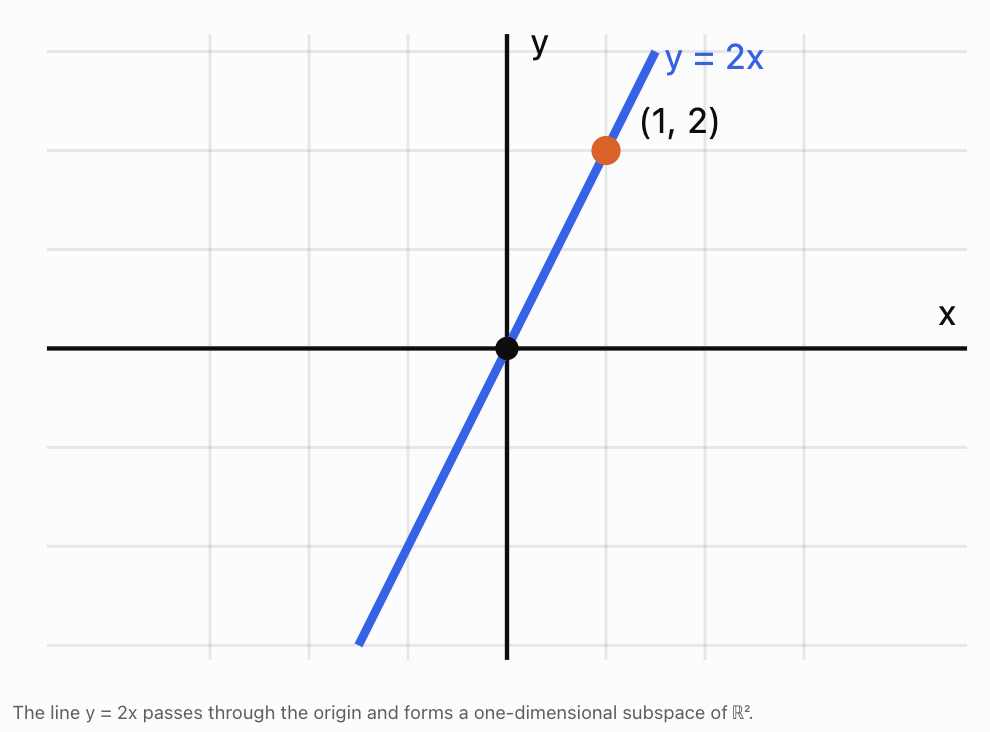
For example, consider all vectors in ℝ² that lie on the line:
y = 2x
These vectors have the form:
where t is any real number.
Equivalently:
This collection forms a subspace of ℝ².
It includes the zero vector when t = 0.
Adding two vectors on the line produces another vector on the line.
Multiplying any vector on the line by a scalar keeps it on the line.
Why Not Every Line Is a Subspace
Consider:
y = 2x + 3
This line does not pass through the origin.
The zero vector (0, 0) does not lie on the line.
Therefore, the line is not a vector subspace of ℝ².
Important principle: Every vector subspace must contain the zero vector.
The Span of a Set of Vectors
The span of a collection of vectors is the set of all possible linear combinations of those vectors.
For vectors u and v:
The span tells us what part of a vector space can be reached using the given vectors.
Example 1: One Vector in Two Dimensions
Suppose:
All scalar multiples of u lie on a line through the origin.
Therefore:
is a line.
Example 2: Two Independent Vectors in Two Dimensions
Suppose:
Any vector:
can be written as:
Therefore:
These two vectors span the entire two-dimensional plane.
Example 3: Two Vectors on the Same Line
Suppose:
Since:
the vectors point along the same line.
Their span is only a line, not the entire plane.
Adding the second vector does not create any new direction.
Linear Independence
Vectors are linearly independent when none of them can be written as a linear combination of the others.
In two dimensions, two nonzero vectors are linearly independent when they do not lie along the same line through the origin.
For example:
are independent.
Neither vector can be obtained by multiplying the other by a scalar.
However:
are dependent because:
Formal Definition
Vectors v₁, v₂, ..., vₙ are linearly independent if the equation:
has only the solution:
This is called the trivial solution.
If another solution exists in which at least one coefficient is nonzero, the vectors are linearly dependent.
Visualising Linear Independence
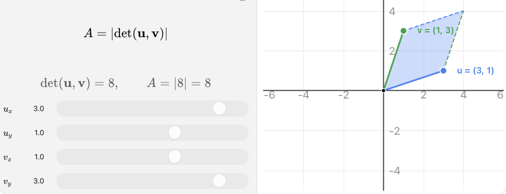
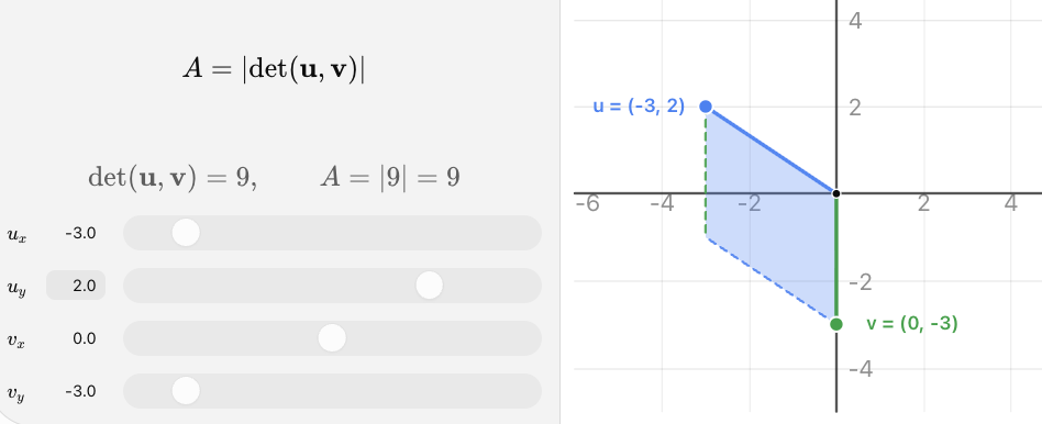
Move the vectors to investigate what happens when they point in different directions or become parallel.
When two vectors in ℝ² are independent, the parallelogram formed by them has nonzero area. When they are dependent, the parallelogram collapses into a line and its area becomes zero.
Worked Example 3: Testing Independence Using a Determinant
Given:
Construct a matrix using the vectors as columns:
Calculate its determinant:
Since the determinant is not zero, the vectors are linearly independent.
Worked Example 4: Identifying Dependent Vectors
Given:
Notice:
Therefore, the vectors are linearly dependent.
We can also check using the determinant:
The zero determinant confirms that the vectors are dependent.
Important: The determinant test applies directly when the vectors form a square matrix, such as two vectors in ℝ² or three vectors in ℝ³. More general collections can be tested using row reduction or the defining equation for linear independence.
Linear Independence in Three Dimensions
In ℝ³, three vectors are linearly independent when none can be expressed as a linear combination of the other two.
For example, the vectors:
are linearly independent.
They point along three distinct coordinate directions.
Together, they span all of ℝ³.
Any vector:
can be expressed as:
However, three vectors that all lie in the same plane through the origin cannot span ℝ³.
They do not provide three independent directions.
Basis Vectors
A basis is a set of vectors that satisfies two conditions:
-
The vectors are linearly independent.
-
The vectors span the entire vector space.
A basis provides a set of fundamental directions from which every vector in the space can be constructed.
The Standard Basis of ℝ²
The standard basis vectors are:
Any vector:
can be written as:
For example:
The Standard Basis of ℝ³
The standard basis is:
Any vector in ℝ³ can be expressed as a linear combination of these three basis vectors.
A Vector Space Can Have Different Bases
The standard basis is not the only possible basis.
For example, consider:
These vectors are linearly independent because:
Since the determinant is nonzero, they form a basis for ℝ².
Worked Example 5: Coordinates in a Different Basis
Express:
using the basis:
We want:
This gives:
a + b = 8
a − b = 2
Add:
2a = 10
a = 5
Then:
b = 3
Therefore:
The coordinates of w in the basis B are:
The vector itself has not changed.
Only the coordinate system used to describe it has changed.
This distinction is important in advanced mathematics, physics, and engineering.
Dimension of a Vector Space
The dimension of a finite-dimensional vector space is the number of vectors in any basis for that space.
Examples:
|
Vector space |
Dimension |
Example basis |
|---|---|---|
|
ℝ¹ |
1 |
(1) |
|
ℝ² |
2 |
(1, 0), (0, 1) |
|
ℝ³ |
3 |
(1, 0, 0), (0, 1, 0), (0, 0, 1) |
|
Polynomials of degree at most 2 |
3 |
1, x, x² |
|
2 × 2 real matrices |
4 |
Four matrices each with one entry equal to 1 and all others 0 |
Why Dimension Matters
Dimension tells us how many independent quantities are needed to describe an object in the space.
For example:
-
A point on a line requires one coordinate.
-
A point in a plane requires two coordinates.
-
A point in ordinary three-dimensional space requires three coordinates.
-
A quadratic polynomial requires three coefficients.
The concept extends to much larger spaces.
A digital image containing 1,000 grayscale pixels can be represented as a vector in ℝ¹⁰⁰⁰.
This is one reason linear algebra is so important in data science and artificial intelligence.
The Role of Matrices in Linear Algebra
Matrices are closely connected to vectors and vector spaces.
A matrix can represent a linear transformation.
A linear transformation is a function T satisfying:
and:
These properties mean that the transformation preserves vector addition and scalar multiplication.
Example: A Linear Transformation
Consider:
This transformation doubles the x-coordinate and triples the y-coordinate.
Its matrix is:
For:
we calculate:
Therefore:
The matrix describes how the transformation acts on vectors.
Matrix Columns and Basis Vectors
An especially important result is that the columns of a transformation matrix describe what happens to the standard basis vectors.
Consider:
Apply A to the first standard basis vector:
Apply A to the second standard basis vector:
The first column of A is the image of the first basis vector.
The second column of A is the image of the second basis vector.
Therefore:
This is a fundamental connection between matrices and linear transformations.
Once we know what a linear transformation does to every vector in a basis, we know what it does to every vector in the space.
Rank and the Number of Independent Directions
The rank of a matrix is the number of linearly independent columns, which is also equal to the number of linearly independent rows.
Rank describes how many independent directions are preserved by a linear transformation.
Worked Example 6: Determining Matrix Rank
Consider:
The second column is twice the first.
Therefore, the columns are linearly dependent.
The matrix has rank 1.
Now consider:
Its determinant is:
Since the determinant is nonzero, the columns are independent.
Therefore:
Geometric Interpretation
A rank-2 transformation in ℝ² preserves two independent directions and maps the plane onto the plane.
A rank-1 transformation in ℝ² maps every vector onto a line through the origin.
A rank-0 transformation maps every vector to the zero vector.
Rank is important when solving systems of equations and analysing datasets.
Linear Algebra and Systems of Equations
Consider:
The columns of A can be interpreted as vectors.
For example:
This means:
The question becomes:
Can the target vector be expressed as a linear combination of the columns of A?
If the columns form a basis for ℝ², every target vector in ℝ² can be represented uniquely.
If the columns are dependent, some target vectors may not be reachable, and others may have infinitely many representations.
Worked Example 7: Solving a System Using Column Vectors
Solve:
2x + y = 5
x + 3y = 7
From the first equation:
y = 5 − 2x
Substitute into the second:
x + 3(5 − 2x) = 7
x + 15 − 6x = 7
−5x = −8
Then:
Therefore:
This means:
The target vector is expressed as a linear combination of two independent column vectors.
Connections to Higher Mathematics
Linear algebra provides the foundation for many advanced mathematical ideas.
Eigenvalues and Eigenvectors
An eigenvector is a nonzero vector whose direction is preserved by a linear transformation, apart from possible reversal.
where λ is an eigenvalue.
Eigenvalues help describe the behaviour of transformations, vibrations, population models, and dynamic systems.
Differential Equations
Systems of differential equations can be written in matrix form.
For example:
Such equations describe how several quantities change together over time.
They are important in physics, engineering, biology, and economics.
Multivariable Calculus
Matrices describe derivatives of functions with multiple inputs and outputs.
The Jacobian matrix organises partial derivatives.
For:
the Jacobian is:
This connects linear algebra with calculus.
Optimisation
Many optimisation problems involve finding the best possible solution under constraints.
Linear algebra is used to represent the constraints and calculate efficient solutions.
Examples include:
-
Minimising production costs.
-
Optimising transport networks.
-
Designing efficient structures.
-
Fitting mathematical models to data.
Data Science and Machine Learning
Large datasets can be represented using matrices.
Rows may represent observations, while columns represent variables.
Linear algebra supports:
-
Linear regression.
-
Principal component analysis.
-
Neural networks.
-
Image recognition.
-
Recommendation systems.
-
Data compression.
Real-World Applications
Robotics and Engineering
Robots use vectors and matrices to represent positions, orientations, and movement. Basis changes allow engineers to convert coordinates between different reference frames.
Computer Graphics
Matrices transform three-dimensional objects through rotations, reflections, scaling, and projections. Graphics software relies on efficient matrix calculations.
Artificial Intelligence
Machine learning systems process large collections of numerical data. Matrix multiplication is a fundamental operation in neural networks and other models.
Structural Engineering
Engineers use matrix methods to calculate forces, displacements, and stresses in buildings and bridges. Rank and independence help determine whether engineering equations provide enough information.
Statistics and Scientific Research
Matrices organise measurements and support regression, covariance analysis, and dimensionality reduction. Independent variables provide distinct information about a system.
Common Mistakes
Mistake 1: Thinking vectors must always represent arrows
Vectors can also be lists of numbers, functions, polynomials, and other mathematical objects.
Mistake 2: Confusing a vector with a scalar
A scalar is a number, while a vector is an element of a vector space.
Mistake 3: Assuming any collection of vectors forms a vector space
A vector space must satisfy specific rules, including closure under addition and scalar multiplication.
Mistake 4: Forgetting the zero vector
Every vector space and subspace must contain the zero vector.
Mistake 5: Assuming every line in ℝ² is a subspace
Only lines passing through the origin are one-dimensional subspaces of ℝ².
Mistake 6: Confusing span with linear independence
Span describes the vectors that can be constructed. Independence describes whether the original vectors contain redundant information.
Mistake 7: Assuming two different vectors are always independent
Two different vectors may still be scalar multiples of one another.
Mistake 8: Confusing a basis with any collection of vectors
A basis must both span the space and be linearly independent.
Mistake 9: Assuming every basis must use standard coordinate vectors
Many different bases can describe the same vector space.
Mistake 10: Confusing dimension with the number of vectors in an arbitrary collection
Dimension is the number of vectors in a basis, not the number of vectors someone happens to list.
Mistake 11: Assuming matrix multiplication is commutative
In general:
AB ≠ BA
Mistake 12: Thinking a matrix is only a rectangular arrangement of numbers
A matrix can represent a linear transformation between vector spaces.
Mistake 13: Assuming every system of equations has exactly one solution
A system may have one solution, no solution, or infinitely many solutions.
Mistake 14: Confusing rank with the total number of rows or columns
Rank counts independent rows or columns.
Key Terms
-
Linear Algebra: Branch of mathematics studying vectors, vector spaces, matrices, and linear transformations.
-
Vector: Element of a vector space that can be added and multiplied by scalars.
-
Scalar: Number used to multiply a vector.
-
Vector Addition: Operation combining two vectors.
-
Scalar Multiplication: Operation multiplying a vector by a scalar.
-
Linear Combination: Sum of scalar multiples of vectors.
-
Vector Space: Collection of vectors satisfying the vector-space axioms.
-
Subspace: Subset of a vector space that is itself a vector space under the same operations.
-
Closure: Property that an operation produces a result within the same set.
-
Zero Vector: Vector that acts as the additive identity.
-
Span: Set of all linear combinations of a collection of vectors.
-
Linear Independence: Property that no vector in a collection can be expressed as a linear combination of the others.
-
Linear Dependence: Property that a nontrivial linear combination of vectors equals the zero vector.
-
Trivial Solution: Solution in which all coefficients are zero.
-
Basis: Linearly independent set of vectors that spans a vector space.
-
Standard Basis: Common coordinate basis using unit vectors along the coordinate axes.
-
Coordinates Relative to a Basis: Scalars used to express a vector as a linear combination of basis vectors.
-
Dimension: Number of vectors in a basis of a finite-dimensional vector space.
-
Linear Transformation: Mapping that preserves vector addition and scalar multiplication.
-
Transformation Matrix: Matrix representing a linear transformation relative to chosen bases.
-
Rank: Number of linearly independent columns or rows of a matrix.
-
Determinant: Scalar associated with a square matrix that can indicate invertibility and signed volume scaling.
-
Invertible Matrix: Square matrix with an inverse.
-
Column Space: Span of the columns of a matrix.
-
Null Space: Set of vectors mapped to zero by a matrix.
-
Eigenvector: Nonzero vector whose image under a transformation is a scalar multiple of itself.
-
Eigenvalue: Scalar associated with an eigenvector under a linear transformation.
-
Jacobian Matrix: Matrix containing first-order partial derivatives.
-
Abstract Mathematics: Study of mathematical structures through general properties and relationships.
Key Takeaways
-
Linear algebra studies vectors, matrices, vector spaces, and linear transformations.
-
Vectors can represent geometric directions, data, functions, and many other mathematical objects.
-
Linear combinations allow new vectors to be constructed from existing vectors.
-
A vector space must satisfy specific rules for addition and scalar multiplication.
-
A subspace is a smaller vector space contained within a larger one.
-
The span of a set of vectors contains every linear combination of those vectors.
-
Linearly independent vectors provide distinct mathematical directions.
-
Linearly dependent vectors contain redundant information.
-
A basis must be both linearly independent and span the entire space.
-
A vector can have different coordinates when expressed in different bases.
-
The dimension of a finite-dimensional vector space equals the number of vectors in any basis.
-
Matrices can represent linear transformations.
-
The columns of a transformation matrix describe the images of the standard basis vectors.
-
Matrix rank describes the number of independent directions represented by a matrix.
-
Linear algebra provides the foundation for advanced calculus, differential equations, optimisation, engineering, and artificial intelligence.
Check Your Understanding
Questions
Question 1: Vector Addition
Given:
Calculate u + v.
Question 2: Scalar Multiplication
Given:
Calculate −3v.
Question 3: Linear Combinations
Given:
Calculate 4u − 2v.
Question 4: Vector Spaces
Explain why ℝ² is a vector space.
Question 5: Subspaces
Determine whether the line:
y = −3x
forms a subspace of ℝ².
Explain your reasoning.
Question 6: Non-Subspaces
Explain why the line:
y = 2x + 5
is not a subspace of ℝ².
Question 7: Span
Describe geometrically the span of:
Question 8: Linear Independence
Determine whether:
are linearly independent.
Question 9: Determinant Test
Determine whether:
are linearly independent.
Question 10: Standard Basis
Express:
as a linear combination of the standard basis vectors of ℝ².
Question 11: Alternative Basis
Given:
Express:
as a linear combination of u and v.
Question 12: Dimension
State the dimension of each space:
a) ℝ²
b) ℝ³
c) Polynomials of degree at most 3
d) All real 2 × 2 matrices
Question 13: Matrix Transformations
Given:
calculate:
Interpret the transformation geometrically.
Question 14: Matrix Rank
Determine the rank of:
Explain your reasoning.
Question 15: Integrated Linear Algebra Challenge
Consider the vectors:
a) Construct a matrix using u and v as columns.
b) Calculate its determinant.
c) Determine whether the vectors are linearly independent.
d) Explain whether the vectors form a basis for ℝ².
e) Express:
as a linear combination of u and v.
f) Explain the geometric meaning of the result.
Fully Worked Answers
Answer 1: Vector Addition
Answer 2: Scalar Multiplication
Answer 3: Linear Combinations
Subtract:
Answer 4: Vector Spaces
ℝ² contains all ordered pairs of real numbers.
Adding two vectors in ℝ² produces another ordered pair of real numbers.
Multiplying a vector by any real scalar also produces another vector in ℝ².
The zero vector is included, and the usual vector-space rules are satisfied.
Therefore, ℝ² is a vector space.
Answer 5: Subspaces
The line is:
y = −3x
Every vector on the line has the form:
The line passes through the origin.
It is closed under vector addition and scalar multiplication.
Therefore:
Answer 6: Non-Subspaces
The line:
y = 2x + 5
does not pass through the origin.
When x = 0:
y = 5
Therefore, the zero vector (0, 0) does not lie on the line.
Since every subspace must contain the zero vector, this line is not a subspace of ℝ².
Answer 7: Span
The vector is:
Its span consists of all scalar multiples:
This produces every point on the line through the origin in the direction (3, 1).
The line has equation:
Therefore, the span is a one-dimensional line through the origin.
Answer 8: Linear Independence
Given:
Notice:
Therefore, the vectors are linearly dependent.
Answer 9: Determinant Test
Construct:
Calculate:
Since the determinant is nonzero, the vectors are linearly independent.
Answer 10: Standard Basis
The standard basis vectors are:
Therefore:
Answer 11: Alternative Basis
We want:
This gives:
a + b = 10
a − b = 4
Add:
2a = 14
a = 7
Then:
b = 3
Therefore:
Answer 12: Dimension
a) ℝ² has dimension 2.
b) ℝ³ has dimension 3.
c) Polynomials of degree at most 3 have basis:
1, x, x², x³
Therefore, the dimension is 4.
d) A real 2 × 2 matrix has four independently selectable entries.
Therefore, the space of all real 2 × 2 matrices has dimension 4.
Answer 13: Matrix Transformations
Calculate:
Geometrically, the transformation stretches the x-coordinate by a factor of 3 and the y-coordinate by a factor of 2.
Answer 14: Matrix Rank
Given:
The second column is twice the first.
Therefore, the columns are linearly dependent.
Since the matrix contains a nonzero column, it has one independent column.
Answer 15: Integrated Linear Algebra Challenge
Part a: Construct the matrix
Using u and v as columns:
Part b: Calculate the determinant
Part c: Linear independence
Since the determinant is nonzero, the vectors are linearly independent.
Part d: Basis
Two linearly independent vectors in ℝ² span the entire plane.
Therefore, u and v form a basis for ℝ².
Part e: Express w as a linear combination
We want:
This gives:
2a + b = 8
a + 3b = 11
From the first equation:
b = 8 − 2a
Substitute:
a + 3(8 − 2a) = 11
a + 24 − 6a = 11
−5a = −13
Then:
Therefore:
Part f: Geometric interpretation
The vectors u and v provide two independent directions in the plane.
By scaling and adding them, we can reach the target vector w.
Because the vectors form a basis, every vector in ℝ² can be expressed uniquely as a linear combination of u and v.
This demonstrates the relationship between linear independence, span, and basis.
Final Reflection
Linear algebra provides a framework for understanding vectors, matrices, and the mathematical spaces in which they operate.
The ideas of linear combinations, span, independence, and basis explain how mathematical objects can be constructed from smaller sets of fundamental elements.
Vector spaces extend these concepts beyond ordinary geometric arrows to functions, polynomials, datasets, and other abstract mathematical structures.
Matrices describe linear transformations, while rank reveals the number of independent directions represented by a transformation.
These foundations connect directly to advanced topics such as eigenvalues, differential equations, multivariable calculus, optimisation, computer graphics, and machine learning.
The central idea is that linear algebra allows us to understand complex mathematical systems by identifying their independent components, describing how those components combine, and studying the transformations that act on them.