Matrix Transformations and Applications
4. Computer Graphics and Robotics
Learning outcomes
- I can explain how matrices are used in computer graphics.
- I can model object transformations.
- I can describe robotic movement using matrices.
- I can analyse simple graphical transformations.
- I can recognise applications in technology.
Introduction
Every time a video game character moves, a 3D model rotates, or a robot arm reaches for an object, mathematics is working behind the scenes.
Computer graphics and robotics rely heavily on matrices to describe positions, movements, rotations, reflections, enlargements, and changes in perspective.
A computer-generated object may contain thousands or millions of points. Rather than calculating the movement of every point separately using different formulas, computers use matrix transformations to apply consistent mathematical operations efficiently.
Similarly, robots use matrices to describe the positions and orientations of their components. When a robotic arm rotates at a joint, the positions of all attached components change. Matrix multiplication allows engineers to calculate these changes systematically.
Matrices are used in:
-
Video games and computer animation.
-
Three-dimensional modelling and rendering.
-
Virtual reality and augmented reality.
-
Industrial robotic arms.
-
Autonomous vehicles and drones.
-
Medical imaging and robotic surgery.
-
Computer vision and object tracking.
-
Satellite navigation and aerospace engineering.
In this lesson, we will investigate how matrices represent graphical transformations, how transformations can be combined, and how similar mathematical techniques are used to control robotic movement.
How Computers Represent Objects
A computer graphic can be represented using a collection of points called vertices.
In two dimensions, each vertex has coordinates:
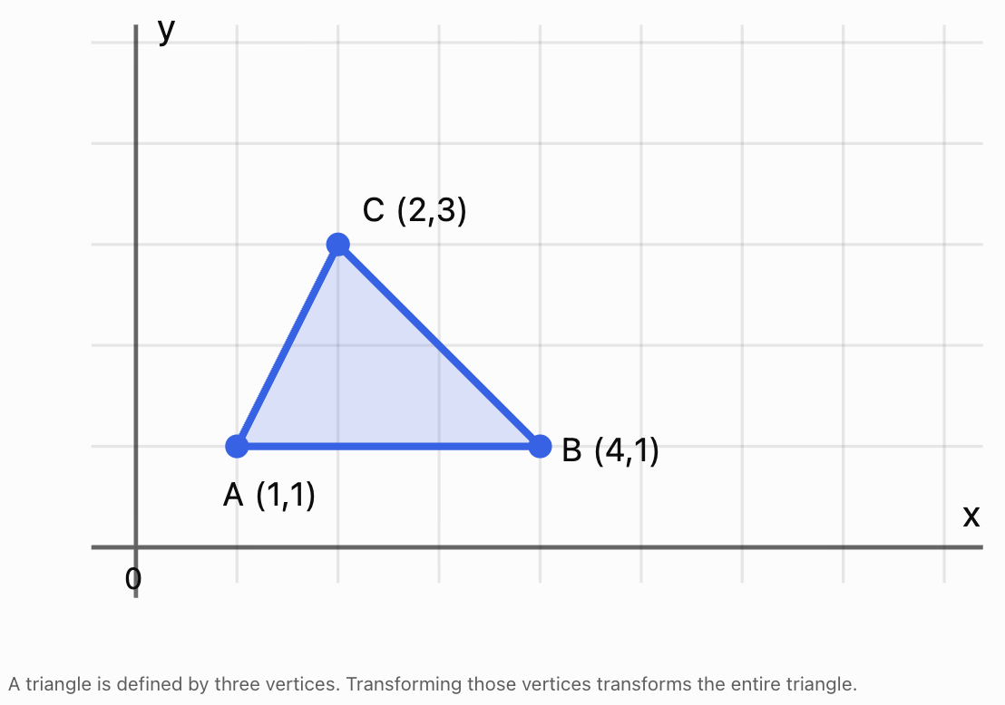
For example, a triangle may have vertices:
A = (1, 1)
B = (4, 1)
C = (2, 3)
These vertices determine the shape of the triangle.
We can organise the coordinates into a matrix:
Each column represents one vertex.
If T is a 2 × 2 transformation matrix, the transformed vertices are:
This means one matrix multiplication can transform every vertex of the object.
For a 3D object, vertices have three coordinates:
A 3 × 3 matrix can then represent rotations, reflections, scaling, and shears in three-dimensional space.
Matrix Transformations in Computer Graphics
A transformation changes the position, size, shape, or orientation of an object.
Common transformations include:
|
Transformation |
Effect |
|---|---|
|
Translation |
Moves an object |
|
Rotation |
Turns an object |
|
Reflection |
Flips an object |
|
Enlargement |
Increases its size |
|
Reduction |
Decreases its size |
|
Shear |
Slants or distorts its shape |
Most of these transformations can be represented by 2 × 2 matrices when they are performed about the origin.
Translations require a different approach, which we will investigate using homogeneous coordinates.
Rotation Matrices
A rotation turns an object through a specified angle about a fixed point.
For a counterclockwise rotation through angle θ about the origin:
For a point P:
Common Rotation Matrices
A 90° counterclockwise rotation:
A 180° rotation:
A 270° counterclockwise rotation:
A clockwise rotation through θ is equivalent to a counterclockwise rotation through −θ.
Worked Example 1: Rotating a Point
Rotate P = (3, 2) by 90° counterclockwise about the origin.
Use:
Then:
Therefore:
The point has rotated 90° counterclockwise while remaining the same distance from the origin.
Worked Example 2: Rotating an Entire Triangle
Consider the triangle:
A = (1, 1)
B = (3, 1)
C = (2, 3)
Its vertex matrix is:
Apply a 90° counterclockwise rotation:
The result is:
Therefore:
A′ = (−1, 1)
B′ = (−1, 3)
C′ = (−3, 2)
The triangle has rotated without changing its side lengths or angles.
Reflection Matrices
A reflection flips an object across a specified line.
Reflection in the x-axis
This maps:
(x, y) → (x, −y)
Reflection in the y-axis
This maps:
(x, y) → (−x, y)
Reflection in the line y = x
This maps:
(x, y) → (y, x)
Worked Example 3: Reflecting a Point
Reflect P = (4, −2) in the y-axis.
The reflected point is (−4, −2).
Reflections preserve lengths and angles but reverse orientation.
Scaling Matrices
Scaling changes the size of an object.
A general two-dimensional scaling matrix is:
where:
-
sₓ is the horizontal scale factor.
-
sᵧ is the vertical scale factor.
If sₓ = sᵧ, the scaling is uniform.
If sₓ and sᵧ are different, the scaling is non-uniform.
Worked Example 4: Non-Uniform Scaling
A point P = (2, 3) is scaled horizontally by factor 3 and vertically by factor 2.
Then:
The new point is (6, 6).
Non-uniform scaling may distort the proportions of an object.
Uniform scaling preserves its shape.
Shear Transformations
A shear transformation slants an object.
A horizontal shear has the form:
This maps:
(x, y) → (x + ky, y)
A vertical shear has the form:
This maps:
(x, y) → (x, kx + y)
Worked Example 5: Horizontal Shear
Apply a horizontal shear with k = 2 to P = (1, 3).
Therefore:
The y-coordinate remains unchanged, while the x-coordinate increases.
Exploring Graphical Transformations
Change the transformation and observe how a square is altered.
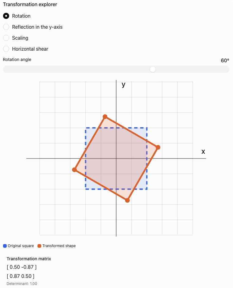
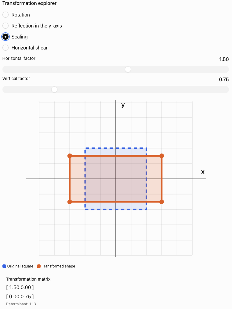
Observe how the determinant relates to the area and orientation of the transformed shape.
Combining Transformations
Computer graphics often requires several transformations to be applied to the same object.
For example, a character may need to:
-
Rotate.
-
Enlarge.
-
Move to a new position.
Matrix multiplication allows these operations to be combined.
Suppose A is applied first, followed by B.
Then:
Therefore:
The order of matrix multiplication is important.
In general:
Worked Example 6: Rotation Followed by Scaling
Consider:
First rotate 90° counterclockwise:
Then scale horizontally by factor 2:
The combined transformation is:
Calculate:
Apply to P:
Reversing the Order
Now scale first and rotate second.
Therefore:
The results differ:
-
Rotation then scaling: (−4, 1)
-
Scaling then rotation: (−2, 2)
This demonstrates why transformation order must be handled carefully.
Translation and Homogeneous Coordinates
A translation moves every point by the same amount.
For a point (x, y), a translation by (a, b) gives:
A standard 2 × 2 matrix cannot represent a nonzero translation because matrix multiplication maps the origin to itself.
Computer graphics solves this problem using homogeneous coordinates.
A two-dimensional point is represented using three coordinates:
A translation becomes:
Then:
This allows translation, rotation, scaling, and other affine transformations to be combined using matrix multiplication.
Worked Example 7: Translating a Point
Translate P = (2, 3) by 4 units right and 2 units down.
Therefore:
a = 4
b = −2
Apply the transformation:
Therefore:
Homogeneous Transformation Matrices
Using homogeneous coordinates, a general two-dimensional affine transformation can be written as:
The upper-left 2 × 2 block describes the linear transformation.
The final column describes translation.
This structure is extremely useful in computer graphics and robotics.
For example, a rotation followed by a translation can be represented using a single 3 × 3 matrix.
Worked Example 8: Rotation and Translation
Rotate a point by 90° counterclockwise, then translate it 5 units right and 2 units up.
The combined matrix is:
Apply it to P = (2, 1):
Therefore:
We can verify the result manually.
Rotate:
(2, 1) → (−1, 2)
Translate:
(−1 + 5, 2 + 2) = (4, 4)
The results agree.
Three-Dimensional Computer Graphics
Realistic computer graphics usually operates in three dimensions.
A 3D point has coordinates:
Three-dimensional rotations can occur around the x-axis, y-axis, or z-axis.
Rotation Around the x-Axis
Rotation Around the y-Axis
Rotation Around the z-Axis
These formulas use the usual right-handed coordinate system and the right-hand rule for positive rotations.
Worked Example 9: Rotating in Three Dimensions
Consider:
Rotate 90° counterclockwise around the z-axis, as viewed from the positive z-axis towards the origin.
Then:
The z-coordinate remains unchanged because the rotation occurs around the z-axis.
How Matrices Are Used in Robotics
Robotics uses many of the same mathematical ideas as computer graphics.
A robot must understand:
-
Where it is located.
-
Which direction it is facing.
-
How its joints are positioned.
-
Where its tools or sensors are located.
-
How to move from one position to another.
Matrices provide a consistent mathematical method for describing these relationships.
Coordinate Frames
A coordinate frame defines a position and orientation from which measurements are made.
A robot may use several coordinate frames:
-
World frame: fixed reference for the environment.
-
Robot base frame: attached to the robot's base.
-
Joint frames: attached to moving joints.
-
Tool frame: attached to the robot's end effector.
The end effector is the part of a robot that performs a task, such as a gripper, welding tool, or surgical instrument.
Transformations allow coordinates to be converted from one frame to another.
Modelling a Simple Robotic Arm
Consider a robotic arm operating in a two-dimensional plane.
The arm has two segments:
-
First segment of length L₁.
-
Second segment of length L₂.
The first joint rotates through angle θ₁.
The second joint rotates through angle θ₂ relative to the first segment.
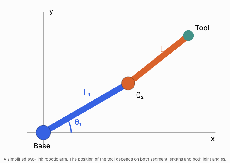
The end effector's position can be calculated using trigonometry.
These equations are examples of forward kinematics.
Forward kinematics calculates the position of the robot's end effector from known joint angles and link lengths.
Worked Example 10: Position of a Robotic Arm
A robot has:
L₁ = 4 m
L₂ = 3 m
θ₁ = 30°
θ₂ = 60°
Calculate the position of the end effector.
Step 1: Calculate the horizontal position.
Using:
cos 30° ≈ 0.866
cos 90° = 0
Therefore:
x = 4(0.866) + 3(0)
x ≈ 3.464 m
Step 2: Calculate the vertical position.
Using:
sin 30° = 0.5
sin 90° = 1
Therefore:
y = 4(0.5) + 3(1)
y = 2 + 3
y = 5 m
Therefore:
The end effector is approximately 3.464 m horizontally and 5 m vertically from the robot's base.
Forward Kinematics Using Matrices
The same robotic arm can be modelled using homogeneous transformation matrices.
For a planar rotation θ followed by movement of length L along the rotated local x-axis:
For a two-link arm:
where:
and:
The total transformation describes the end effector's position and orientation relative to the robot's base.
The resulting matrix is:
where:
x = L₁ cos θ₁ + L₂ cos(θ₁ + θ₂)
y = L₁ sin θ₁ + L₂ sin(θ₁ + θ₂)
This method becomes especially useful for robots with many joints.
Instead of constructing a separate set of trigonometric equations for every possible configuration, engineers multiply transformation matrices representing individual joints.
Inverse Kinematics
Inverse kinematics works in the opposite direction from forward kinematics.
Forward kinematics asks:
Given the joint angles, where is the end effector?
Inverse kinematics asks:
Given a desired end-effector position, what joint angles are required?
For example, a robotic arm may need to pick up an object at coordinates (5, 2).
The robot must calculate joint angles that position its gripper at that location.
Inverse kinematics is generally more difficult because:
-
Some target positions may be unreachable.
-
Multiple joint configurations may reach the same position.
-
Some configurations may cause collisions.
-
Joint movement may be limited.
-
Numerical methods may be required for complicated robots.
Simple Reachability Example
A robotic arm has two segments:
L₁ = 4 m
L₂ = 3 m
The maximum distance it can reach from its base is:
L₁ + L₂ = 7 m
The minimum distance for a freely rotating two-link planar arm is:
|L₁ − L₂| = 1 m
Therefore, without joint restrictions or obstacles, the end effector can reach positions whose distance r from the base satisfies:
A target 8 m from the base is unreachable.
A target 5 m from the base may be reachable.
This is an important practical constraint in robot design.
Three-Dimensional Robotics
Industrial robots usually move in three-dimensional space.
A robotic tool must have both a position and an orientation.
Position describes where the tool is located:
(x, y, z)
Orientation describes how the tool is rotated relative to a reference frame.
Robotics commonly uses a 4 × 4 homogeneous transformation matrix:
The upper-left 3 × 3 block is a rotation matrix R.
The final column contains the translation coordinates.
This is often written more compactly as:
where:
-
R describes orientation.
-
t describes position.
-
H combines rotation and translation.
A valid 3D rotation matrix satisfies:
RᵀR = I
det(R) = 1
Worked Example 11: Transforming a 3D Point
A robot rotates a point by 90° about the z-axis, then translates it by:
(4, 2, 3)
The transformation matrix is:
The original point is:
P = (2, 1, 5)
In homogeneous coordinates:
Calculate:
The resulting coordinates are:
x′ = −1 + 4 = 3
y′ = 2 + 2 = 4
z′ = 5 + 3 = 8
Therefore:
This is how a robot can convert the position of an object from one coordinate frame into another.
Computer Graphics: From a 3D Model to a Screen
A three-dimensional object cannot be displayed directly on a flat screen without a projection.
Computer graphics uses a sequence of transformations to convert 3D coordinates into screen coordinates.
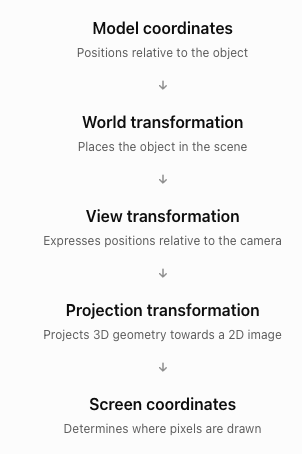
Using column vectors, a typical transformation pipeline is:
where:
-
M is the model matrix.
-
V is the view matrix.
-
P_proj is the projection matrix.
-
P_model is the original point in homogeneous coordinates.
The result is in clip coordinates. For perspective projection, the computer subsequently performs a perspective division and viewport mapping to obtain screen coordinates.
Orthographic and Perspective Projection
Orthographic projection
Parallel lines remain parallel, and distant objects do not appear smaller simply because of their distance.
Perspective projection
Objects farther from the camera appear smaller, producing a more realistic sense of depth.
These projection methods are used in computer-aided design, architectural drawings, video games, and animation.
Analysing Graphical Transformations Using Determinants
The determinant of a transformation matrix reveals useful geometric information.
For a 2 × 2 matrix A:
The sign of the determinant indicates whether orientation is preserved or reversed.
|
Determinant |
Interpretation |
|---|---|
|
det(A) > 0 |
Orientation preserved |
|
det(A) < 0 |
Orientation reversed |
|
det(A) = 0 |
Area collapses to zero |
|
|det(A)| = 1 |
Area preserved |
|
|det(A)| > 1 |
Area enlarged |
|
0 < |det(A)| < 1 |
Area reduced |
Worked Example 12: Analysing a Transformation
Consider:
Calculate:
det(A) = 2(3) − 1(0)
= 6
Therefore:
-
Areas are multiplied by 6.
-
Orientation is preserved.
-
The transformation is invertible.
If a shape originally has an area of 5 cm², its transformed area is:
5 × 6 = 30 cm²
This provides a useful way to check whether a graphical transformation behaves as expected.
Real-World Applications in Technology
Video Games and Animation
Matrices control the positions, rotations, and sizes of characters, objects, cameras, and virtual environments. A character's limbs can be positioned using linked transformations, similar to a robotic arm.
Augmented Reality
Virtual objects are positioned relative to the real environment using transformations that account for the camera's position and orientation.
Medical Robotics
Robotic surgical systems use coordinate transformations to help position instruments accurately. Sensor measurements and control systems provide additional information needed for safe movement.
Autonomous Vehicles and Robots
Robots combine coordinate transformations with sensor data to estimate positions, construct maps, detect obstacles, and plan movement.
Computer-Aided Design
Engineers use transformations to position components, construct assemblies, examine designs, and visualise objects from different viewpoints.
Evaluating Matrix-Based Models
Matrix models are powerful, but real-world graphics and robotics involve additional complexities.
Numerical Accuracy
Computers usually store decimal values with limited precision.
Repeated transformations can introduce small rounding errors.
For example, repeatedly rotating an object through many small angles may eventually produce a slight numerical difference from the expected position.
Physical Constraints
A mathematical transformation may describe a position that a robot cannot physically reach.
Robots have:
-
Limited joint rotation.
-
Maximum extension lengths.
-
Motor speed limits.
-
Load restrictions.
-
Collision constraints.
Coordinate Conventions
Different graphics and robotics systems may use different conventions.
These include:
-
Left-handed or right-handed coordinate systems.
-
Row vectors or column vectors.
-
Different axis orientations.
-
Different rotation orders.
-
Degrees or radians.
A transformation must be interpreted using the conventions of the system.
Model Validation
Engineers verify transformations by checking:
-
Whether calculated positions agree with measured positions.
-
Whether distances and angles are preserved when expected.
-
Whether the transformation matrix is valid.
-
Whether movement remains within physical limits.
-
Whether numerical errors are acceptably small.
Common Mistakes
Mistake 1: Multiplying transformation matrices in the wrong order
Matrix multiplication is generally not commutative. Rotation followed by scaling may produce a different result from scaling followed by rotation.
Mistake 2: Confusing clockwise and counterclockwise rotations
The standard 2D rotation matrix uses positive angles for counterclockwise rotation.
Mistake 3: Forgetting that a 2 × 2 matrix cannot represent a nonzero translation
Use homogeneous coordinates and a 3 × 3 matrix for 2D translation.
Mistake 4: Confusing horizontal and vertical scaling factors
The first diagonal entry scales x, while the second scales y.
Mistake 5: Assuming all transformations preserve distances
Rotations and reflections preserve distances, but general scaling and shearing do not.
Mistake 6: Ignoring the centre of rotation
A standard rotation matrix rotates about the origin. Rotation about another point requires translations as well.
Mistake 7: Confusing local and global coordinates
A robot joint's local coordinates may differ from coordinates measured relative to the robot's base.
Mistake 8: Treating the second robot joint angle as an absolute angle
In a standard two-link robotic arm, θ₂ is measured relative to the first link, so the second link's absolute orientation is θ₁ + θ₂.
Mistake 9: Assuming every target position is reachable
A robot's link lengths and joint limits restrict its workspace.
Mistake 10: Forgetting to check matrix dimensions
A transformation matrix must have compatible dimensions with the vector or matrix it transforms.
Mistake 11: Misinterpreting determinants
The absolute determinant gives area scaling in 2D, while the sign indicates orientation.
Mistake 12: Confusing a model with physical reality
Robotic movement also depends on motors, sensors, forces, and environmental conditions.
Key Terms
-
Computer Graphics: Creation and manipulation of visual images using computers.
-
Vertex: Point defining part of a geometric object.
-
Transformation Matrix: Matrix used to change coordinates or geometric properties.
-
Translation: Movement of an object by a fixed displacement.
-
Rotation: Turning an object around a point or axis.
-
Reflection: Flipping an object across a line or plane.
-
Scaling: Changing the size of an object.
-
Uniform Scaling: Scaling by the same factor in every direction.
-
Non-Uniform Scaling: Scaling by different factors in different directions.
-
Shear: Transformation that slants an object.
-
Homogeneous Coordinates: Extended coordinate representation that allows translations to be combined with linear transformations using matrices.
-
Affine Transformation: Transformation combining linear operations and translation.
-
Composite Transformation: Combination of multiple transformations.
-
Rotation Matrix: Matrix representing rotation through a specified angle.
-
Determinant: Scalar describing geometric scaling and orientation properties.
-
Orientation: Directional alignment of an object or coordinate frame.
-
Coordinate Frame: Reference system used to describe positions and orientations.
-
World Coordinates: Coordinates relative to a fixed global reference.
-
Local Coordinates: Coordinates relative to an object or component.
-
End Effector: Working tool or terminal component of a robot.
-
Joint Angle: Angle describing the rotation of a robotic joint.
-
Forward Kinematics: Calculation of tool position and orientation from joint variables.
-
Inverse Kinematics: Calculation of joint variables needed to reach a desired position or orientation.
-
Workspace: Region a robot can reach.
-
Transformation Pipeline: Sequence of coordinate transformations used in graphics.
-
View Matrix: Matrix expressing coordinates relative to a camera.
-
Projection Matrix: Matrix used to project 3D geometry for display.
-
Orthographic Projection: Projection without perspective size reduction.
-
Perspective Projection: Projection in which distant objects appear smaller.
-
Computer Vision: Field involving the interpretation of images and visual data.
-
Robotic Manipulator: Robot designed to position and move objects or tools.
Key Takeaways
-
Computer graphics uses matrices to represent and transform objects.
-
Vertices can be organised into matrices so many points can be transformed simultaneously.
-
Rotation, reflection, scaling, and shear can be represented using 2 × 2 matrices in two dimensions.
-
Homogeneous coordinates allow translation to be represented using matrix multiplication.
-
Composite transformations are calculated by multiplying matrices in the correct order.
-
Transformation order can change the final result.
-
Three-dimensional graphics uses matrices to rotate and position objects in space.
-
Robotics uses transformation matrices to describe positions and orientations of robot components.
-
Forward kinematics calculates tool positions from joint angles.
-
Inverse kinematics calculates joint angles needed to reach target positions.
-
Determinants reveal geometric scaling and orientation.
-
Coordinate transformations are essential in animation, computer-aided design, autonomous systems, and robotics.
-
Mathematical results must be checked against physical constraints and real-world measurements.
Check Your Understanding
Questions
Question 1: Computer Graphics
Explain why matrices are useful when transforming objects containing many vertices.
Question 2: Rotation
Rotate P = (4, 2) by 90° counterclockwise about the origin.
Question 3: Reflection
Reflect P = (−3, 5) in the x-axis.
Question 4: Scaling
Scale P = (2, −4) horizontally by factor 3 and vertically by factor 0.5.
Question 5: Shear
Apply a horizontal shear with k = 2 to P = (3, 2).
Question 6: Transformation Order
A point P = (1, 2) is rotated 90° counterclockwise, then scaled uniformly by factor 3.
Find the final coordinates.
Question 7: Homogeneous Translation
Translate P = (−2, 5) by 4 units right and 3 units down using a homogeneous transformation matrix.
Question 8: Combined Transformation
A point P = (2, 1) is rotated 90° counterclockwise and then translated 3 units right.
Construct the combined homogeneous transformation matrix and find P′.
Question 9: Three-Dimensional Rotation
Rotate P = (1, 3, 2) by 90° about the z-axis.
Question 10: Determinants
A transformation matrix is:
Determine the area scale factor.
Question 11: Robotic Arm
A two-link robotic arm has:
L₁ = 5 m
L₂ = 3 m
θ₁ = 0°
θ₂ = 90°
Calculate the end effector's position.
Question 12: Reachability
A robotic arm has segment lengths 6 m and 4 m.
Assuming unrestricted planar revolute joints, determine its minimum and maximum reachable distances from the base.
Question 13: Forward and Inverse Kinematics
Explain the difference between forward kinematics and inverse kinematics.
Question 14: Technology Applications
Describe two practical applications of transformation matrices in technology.
Question 15: Integrated Challenge
A triangle has vertices:
A = (1, 1)
B = (3, 1)
C = (2, 4)
The triangle undergoes the following transformations:
-
A 90° counterclockwise rotation about the origin.
-
A horizontal enlargement by factor 2.
-
A translation 4 units right and 1 unit up.
a) Write the rotation matrix.
b) Write the scaling matrix.
c) Construct the combined 3 × 3 homogeneous transformation matrix.
d) Calculate the final coordinates of all three vertices.
e) Calculate the determinant of the linear part of the transformation.
f) Determine the area scale factor.
g) Explain whether the transformation preserves orientation.
Fully Worked Answers
Answer 1: Computer Graphics
Matrices allow the same transformation to be applied systematically to many vertices.
If V contains the coordinates of an object and T is a transformation matrix:
V′ = TV
This allows an entire object to be rotated, reflected, scaled, or sheared using matrix multiplication.
Answer 2: Rotation
Answer 3: Reflection
Reflection in the x-axis:
(x, y) → (x, −y)
Therefore:
Answer 4: Scaling
Answer 5: Shear
Horizontal shear:
x′ = 3 + 2(2) = 7
y′ = 2
Answer 6: Transformation Order
Start:
P = (1, 2)
Rotate 90° counterclockwise:
(1, 2) → (−2, 1)
Scale uniformly by factor 3:
(−2, 1) → (−6, 3)
Answer 7: Homogeneous Translation
The translation is:
a = 4
b = −3
Therefore:
Apply to:
Answer 8: Combined Transformation
Rotation matrix in homogeneous coordinates:
Translation matrix:
Combined matrix:
Apply to P = (2, 1):
Answer 9: Three-Dimensional Rotation
For a 90° rotation about the z-axis:
(x, y, z) → (−y, x, z)
Therefore:
(1, 3, 2) → (−3, 1, 2)
Answer 10: Determinants
Calculate:
det(A) = 3(2) − 0
= 6
Therefore:
Areas become six times as large.
Answer 11: Robotic Arm
Given:
L₁ = 5
L₂ = 3
θ₁ = 0°
θ₂ = 90°
Horizontal position:
x = 5 cos 0° + 3 cos 90°
x = 5(1) + 3(0)
x = 5
Vertical position:
y = 5 sin 0° + 3 sin 90°
y = 5(0) + 3(1)
y = 3
Answer 12: Reachability
Maximum reach:
L₁ + L₂ = 6 + 4 = 10 m
Minimum reach:
|L₁ − L₂| = |6 − 4| = 2 m
Therefore:
The arm can reach points whose distance from the base lies between 2 m and 10 m, assuming no joint limits or obstacles.
Answer 13: Forward and Inverse Kinematics
Forward kinematics calculates the end effector's position and orientation from known joint angles and link lengths.
Inverse kinematics calculates the joint angles required to reach a desired position or orientation.
Forward kinematics usually gives a direct calculation.
Inverse kinematics may have multiple solutions, one solution, or no solution.
Answer 14: Technology Applications
Application 1: Video Games
Transformation matrices move, rotate, and scale game objects and characters.
Application 2: Industrial Robotics
Transformation matrices calculate the positions and orientations of robotic arms, grippers, and tools.
Other valid examples include computer-aided design, augmented reality, medical robotics, and autonomous navigation.
Answer 15: Integrated Challenge
Original vertices:
A = (1, 1)
B = (3, 1)
C = (2, 4)
Part a: Rotation matrix
Part b: Scaling matrix
Horizontal enlargement by factor 2:
Part c: Combined homogeneous matrix
First rotate, then scale, then translate.
Homogeneous rotation:
Homogeneous scaling:
Translation:
The combined transformation is:
First:
Then:
Part d: Final coordinates
For A = (1, 1):
x′ = −2 + 4 = 2
y′ = 1 + 1 = 2
A′ = (2, 2)
For B = (3, 1):
x′ = −2 + 4 = 2
y′ = 3 + 1 = 4
B′ = (2, 4)
For C = (2, 4):
x′ = −8 + 4 = −4
y′ = 2 + 1 = 3
C′ = (−4, 3)
Therefore:
Part e: Determinant
The linear part is:
Calculate:
det(A) = 0(0) − (−2)(1)
Part f: Area scale factor
The area scale factor is:
|det(A)| = 2
Therefore, the transformed triangle has twice the original area.
As an additional check, the original triangle has base 2 and height 3:
Area = 1/2 × 2 × 3 = 3 square units
The transformed area is:
2 × 3 = 6 square units
Part g: Orientation
Since:
det(A) = 2 > 0
the transformation preserves orientation.
The rotation preserves orientation, the positive scaling preserves orientation, and translation does not change orientation.
Final Reflection
Matrices provide a common mathematical language for computer graphics and robotics.
In computer graphics, transformation matrices allow objects to be rotated, reflected, scaled, sheared, and translated. Homogeneous coordinates make it possible to combine these operations into a single matrix, while three-dimensional transformations allow virtual objects to be positioned and displayed from different viewpoints.
In robotics, matrices describe the positions and orientations of moving components. Forward kinematics allows engineers to calculate where a robot's tool will move, while inverse kinematics helps determine how joints must move to reach a target.
The same mathematical principles therefore connect animated characters, virtual environments, industrial machinery, autonomous vehicles, and medical robots.
The central idea is that matrices provide an efficient, systematic way to describe and combine movements in both virtual and physical space.